ABSTRACT
YIN, YUANYUAN. Calculation of Membrane Protein Structures in Oriented-Sample NMR and Their Validation using Rosetta. (Under the direction of Dr. Alexander A. Nevzorov).
Membrane proteins encode about 30% of all eukaryotic genomes and constitute the
majority of current drug targets. However, only 2% of solved protein structures in Protein
Data Bank are membrane proteins. To contribute to this outstanding problem, we have
developed a computational methodology for calculating membrane protein structures from
oriented sample solid-state NMR. We have demonstrated the feasibility of obtaining
atomic-resolution three-dimensional backbone structures of membrane proteins solely from the
heteronuclear spin-spin dipolar couplings. We have further validated the calculated structures
and determined their optimal immersion depth in the heterogeneous membrane-aqueous
environment by combining the above structural fitting method and the Rosetta structure
predicting package. Extension of this research include elucidation of the oligomerization
states of homomeric protein assemblies by simultaneously utilizing solid-state NMR
© Copyright 2013 by Yuanyuan Yin
Calculation of Membrane Protein Structures in Oriented-Sample NMR and Their Validation using Rosetta
by Yuanyuan Yin
A dissertation submitted to the Graduate Faculty of North Carolina State University
in partial fulfillment of the requirements for the degree of
Doctor of Philosophy
Chemistry
Raleigh, North Carolina
2013
APPROVED BY:
_______________________________ ______________________________ Alexander A. Nevzorov Alex I. Smirnov
Chair of Advisory Committee
ii
DEDICATION
iii
BIOGRAPHY
Yuanyuan Yin was born on July 23, 1984, the hottest day of that year, in Tianjin, China.
After six years study at Tianjin Shiyan Elementary School, she passed the specialized
qualification exam and started her five years middle-high school life at Tianjin Yaohua High
School in 1997. Here, she competed but also made lifetime friends with many awesome
people.
In 2002, she attended University of Science and Technology of China (USTC) in Hefei,
Anhui, China and chose chemical physics as the major. In 2005 summer, she began her
undergraduate thesis research in Dr. Guangzhao Zhang’s group at National Laboratory for
Physical Sciences and Microscale. With the encouragement and support from Dr. Zhang, she
obtained a large amount access to both chemical and instrument resources in the laboratory,
succeeded in accomplishing her thesis and awarded Outstanding Dissertation. Tianjin
Yaohua High School also received a Letter of Thanks from University of Science and
Technology of China with affirmation of her performance as an undergraduate student.
In August 2006, she enrolled as a graduate student in department of chemistry at North
Carolina State University (NCSU) in Raleigh, North Carolina. After working on dendrimer
synthesis for two years, she joined Dr. Alexander A. Nevzorv’s group and began her research
on development of methodology in membrane protein structure determination. With the
guidance and advice of Dr. Nevzorov, she passed the preliminary oral qualification in six
months. Now four years passed, she is going to defense and complete her Ph.D. degree study.
iv Although her work is about science, she always cannot help thinking about fortune. If she did
not write USTC in her application form, if she switched to another major in her second year
at USTC, if she picked another graduate school offer….. Maybe her life would be totally
different, but if so, how would her life be?
After graduation, she would like to pursue an industrial or an academic career in Houston,
Texas, where driving in snow would not be a concern anymore. Though this would not be an
easy journey, she will keep her motto Never Say Never in mind. Please bless her.
v
ACKNOWLEDGMENTS
I would like to thank, first and foremost, my advisor Alexander A. Nevzorov for giving me
the great opportunity to pursue my doctoral dissertation under his direction. His enthusiasm
about science has inspired me and shaped my career as a scientist. Alex has a beautiful mind
and a great sense of scientific insight and intuition. He can always find a way to overcome
the challenge that seemed to hinder my research. When I encountered obstacles, he was very
patient, understanding, and willing to provide guidance when needed. He also gave me a
great degree of freedom to try my own ideas and learn new programming languages with
which I learned to think and work independently. I am grateful to all these years working in
his group and none of my projects could have been accomplished without his advice. I would
like to thank colleagues at the Nevzorov group, with whom I shared challenges, experiences,
and successes. I would like to thank my dissertation committee members Alex I. Smirnov,
Mike H. Whangbo, Jerry L. Whitten and Stefan Franzen for their great advice and
suggestions. Without the great resource provided by North Carolina State University,
Department of Chemistry and High Performance Computing Center, work in this dissertation
would not be possible. I am also grateful to the great friends in NCSU who have made
graduate school a memorable and enjoyable journey. Last but definitely not least, I would
like to thank my parents, Weidong Yin and Yumin Zhang, for believing in me and loving me
for whoever I am. They have always been there, supporting and encouraging me. I would like
vi
TABLE OF CONTENTS
LIST OF TABLES ... viii
LIST OF FIGURES ... ix
Chapter 1 Introduction ... 1
1.1 Introduction to Membrane Proteins ... 1
1.2 Protein Structure and Folding ... 4
1.2.1 Geometry of Polypeptide Chains ... 4
1.2.2 Hydrophobicity of Amino Acid Residues ... 7
1.2.3 Molecular Modeling using Rosetta Software Package ... 7
1.2.4 Rosetta Sampling Algorithm ... 9
1.2.5 Rosetta Scoring Function ... 10
1.2.6 Assessment of Model Quality ... 13
1.3 Solid-State NMR Studies of Membrane Proteins ... 14
1.3.1 Basic Principles of NMR ... 14
1.3.2 Magic Angle Spinning NMR ... 16
1.3.3 Oriented Solid-State NMR ... 17
1.3.4 Structural Fitting using PISEMA ... 20
1.3.5 Analytical Framework for Solid-State NMR Observables in Torsion-Angle Space ... 21
1.4 Prediction of Helical Membrane Proteins Structures using Rosetta ... 26
1.4.1 De Novo Prediction using Membrane Ab Initio in Rosetta ... 26
1.4.2 High-Resolution Prediction using Adapted All-Atom Energy Function ... 28
1.5 Research Summary ... 29
Chapter 2 Structure Determination in “Shiftless” Solid State NMR of Oriented Protein Samples ... 48
2.1 Introduction ... 48
2.2 NMR Observables in the Spherical Basis and the Algorithm... 52
2.3 Results and Discussion ... 59
2.3.1 Structural Fitting of Simulated Three-Dimensional Spectra with 15N CSA, and 1 H-15 N and 1H-13C Dipolar Couplings ... 59
2.3.2 Structural Fitting of the Three-Dimensional “Shiftless” Spectra with 1H-15N, 1 H-13 C and 13C-15N Dipolar Couplings ... 60
2.3.3 Structural Fitting of Four-Dimensional Data with 1H-15N, 1H-13C, 13C-15N and 13 C’-15N Dipolar Couplings ... 61
2.3.4 Structural Fitting of a Helical Hairpin Derived from Bacteriorhodopsin ... 63
2.4 Conclusions ... 65
Chapter 3 Validation of SSNMR Structures using Rosetta ... 75
3.1 Introduction ... 75
3.2 Application of Membrane Ab Initio Protocol in Rosetta ... 75
vii 3.2.2 Membrane Ab Initio Calculation of Mercuric Ion Transport Proteins (MerF,
MerFt) ... 78
3.2.2.1 Membrane Ab Initio Calculation of MerF (2LJ2) ... 79
3.2.2.2 Membrane Ab Initio Calculation of MerFt (2H3O) ... 80
3.2.2.3 Comparison of Structure Prediction from Different OCTOPUS Topology Files ... 81
3.2.2.4 Effect of Hydrogen Bonding on Conformation Prediction of Transmembrane Helices ... 83
3.3 Structure Validation by PISEMA Back-Calculation ... 84
3.4 Determination of Transmembrane Helices Embedding Positions in Membrane.... 87
3.5 Conclusions ... 91
Chapter 4 Future Directions ... 114
4.1 Homomeric Ion Channels ... 114
4.2 Application of Symmetry Docking to M2 (2L0J)... 115
Chapter 5 Conclusions ... 124
REFERENCES ... 126
APPENDICES ... 141
Appendix A ... 142
Appendix B ... 153
viii
LIST OF TABLES
Table 3.1 Modified OCTOPUS topologies for MerFt (residue 27-70). ... 111
Table 3.2 15N CSA and 1H-15Ndipolar coupling frequencies of MerFt (residue 27-68) .. 112
Table 3.3 Distance constraints used in calculated MerFt structures screening ... 113
Table 4.1 Summary of symmetry docking results for 2L0J... 121
Table 4.2 Summary of symmetry docking results for helical part of 2L0J. ... 122
Table 4.3 Summary of distances measured in native structure, simulated whole structure and
ix
LIST OF FIGURES
Figure 1.1 Schematic representation of the structure types of transmembrane proteins . 30
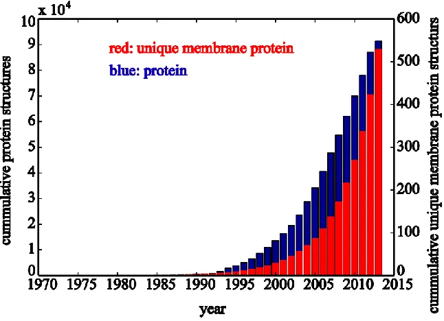
Figure 1.2 Yearly growth of all protein structures and unique membrane protein structures. ... 31
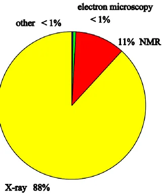
Figure 1.3 Distribution of all experimental methods used in protein structural studies. . 32
Figure 1.4 Representation of the unit of peptide backbone. ... 33
Figure 1.5 Resonance forms of the peptide group. ... 34
Figure 1.6 Trans and cis isomers of the peptide plane. ... 35
Figure 1.7 Representation of torsion angles and , respectively. ... 36
Figure 1.8 Torsion angles / definition. ... 37
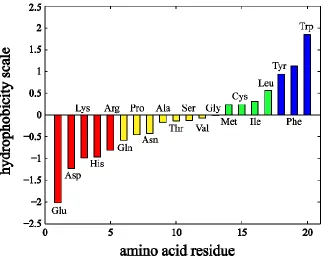
Figure 1.9 Experimentally determined hydrophobicity scale for amino acids. ... 38
Figure 1.10 Rosetta general sampling algorithm. ... 39
Figure 1.11 Splitting of nuclei spin states in an external magnetic field B0 when the angular momentum quantum number I equals ½ (A) and I equals 1 (B). ... 40
Figure 1.12 Nuclear energy levels in an external magnetic field B0 when the angular momentum quantum number I equals ½... 41
Figure 1.13 Schematic Diagram of magic angle spinning solid state NMR. ... 42
Figure 1.14 Representation of a uniaxially oriented membrane protein sample in lipid bilayer. ... 43
Figure 1.15 PISA wheel patterns as a function of tilt angle. ... 44
x Figure 1.17 Membrane definition in OCTOPUS method. ... 46
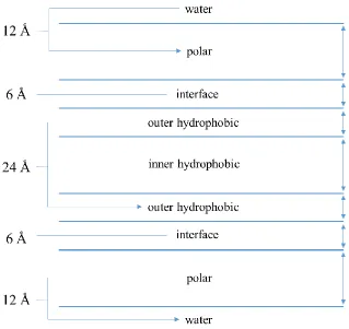
Figure 1.18 Definition of membrane layers in Rosetta membrane ab initio protocol. .... 47
Figure 2.1 Local molecular frame associated with a peptide plane. ... 66
Figure 2.2 Normalized Ramachandran plots for different residue types. ... 67
Figure 2.3 A flowchart for the structural fitting algorithm. ... 68
Figure 2.4 Structural fitting of the simulated three-dimensional solid-state NMR spectrum of
protein G obtained from PDB coordinates 2GB1. ... 69
Figure 2.5 (A) Two-dimensional projection of the simulated spectra (circles) with the same
dimensions as in Fig. 2.4 with 15N CSA input data randomly varied within 1 ppm for each
simulation. (B) Back-calculated structures deviate substantially for each simulation. .. 70
Figure 2.6 (A) Structural fitting of simulated three-dimensional “shiftless” solid-state NMR
spectra and histogram of the RMSDs. (B) The root-mean square deviations (in Hz) at each
residue. ... 71
Figure 2.7 (A) Structural fitting of simulated four-dimensional data for protein G. (B) The
root-mean square deviations (in Hz) at each residue for 1000 fits. ... 72
Figure 2.8 (A) and (B): Histograms of the RMSDs of 1000 back-calculated structures
obtained from three-dimensional “shiftless” solid state NMR spectra of protein G (2GB1)
with a tolerance of 25 Hz (A) and 50 Hz (B). (C) and (D): Histograms of the RMSDs for the
structures satisfying the distance restraints between the Ca carbons of residues Ile6 and
Thr53, and of residues Glu15 and Thr44 for the 25 Hz tolerance (C) and 50 Hz tolerance (D)
xi Figure 2.9 (A) Structural fitting of simulated three-dimensional “shiftless” spectra of two
transmembrane α-helices (residues 104 to 155) of bacteriorhodopsin. (B) The mean of the
deviation (in Hz) at each residue for 100 calculated structures. (C) When the initial structure
is rotated by about 90 degrees, with the tolerance of 25Hz, about 60% of the RMSDs for the
back-calculated structures are more than 5Å. (D) The rms deviation (in Hz) at each residue
for 100 calculated structures. ... 74
Figure 3.1 Structure prediction. (A) 1C3WD (B) 1C3WE (C) 1PY6 ... 93
Figure 3.2 The products of the mer operon(s). ... 94
Figure 3.3 The membrane ab initio energy versus RMSD for MerF. ... 95
Figure 3.4 The membrane ab initio energies calculated with original OCTOPUS topology versus RMSD for MerFt. ... 96
Figure 3.5 The membrane ab initio energies calculated with modified OCOTPUS topology versus RMSD for MerFt. ... 97
Figure 3.6 (Left) The membrane ab initio energy calculated with a series of modified OCOTPUS predicted topology versus RMSD plot for MerFt. (Right) The lowest energy model predicted with each modified OCTOPUS topology ... 98
Figure 3.7 Tendency of RMSDs of MerFt structures predicted by membrane ab initio protocol in Rosetta3.4 along the change of the weight for the hydrogen bonding potential. 101 Figure 3.8 Schematic diagram of membrane rotation. ... 102
Figure 3.9 Comparison of experimental data from solid state NMR experiments and
xii Figure 3.10 Schematic diagram for translation of an NMR-derived structure across lipid
bilayer along the orientation of membrane normal. ... 104
Figure 3.11 Change in all-atom energy of 5-helix 1C3WD along z-axis. ... 105
Figure 3.12 Change in all-atom energy of 2-helix 1C3WE along z-axis. ... 106
Figure 3.13 Change in all-atom energy of bacteriophage Pf1 (2KSJ) along z-axis. ... 107
Figure 3.14 Change in all-atom energy of calculated MerFt along z-axis. ... 108
Figure 3.15 Comparison between experimental data and back-calculated frequencies for 15N CSA and 1H-15N dipolar coupling... 109
Figure 3.16 Summary of MolProbity results for MerFt (2H3O) (top), MerF (2LJ2) (middle), and the partial structure in 2LJ2 with the same sequence as 2H3O (bottom)... 110
Figure 4.1 Symmetry docking results for 2L0J. ... 117
Figure 4.2 Symmetry docking results for helical part of 2L0J. ... 118
Figure 4.3 Illustration of h1A30_h2I35 and h1I35_h2A30 distances measured in PyMOL. 119 Figure 4.4 (A) and (B): Histogram of distances between Ala30 on helix 1 and Ile35 on helix 2. (C) and (D): Histogram of distances between Ile35 on helix 1 and Ala30 on helix 2. 120 Figure A.1 Effect of the variations in the principal components of the 15N CSA tensor on the observed CSA values for protein G. ... 147
Figure A.2 Effect of the orientation of the 15N CSA tensor on the observed CSA values for protein G. ... 148
xiii Figure A.4 Histograms of the RMSDs of 1000 back-calculated structures by simulating
four-dimensional “shiftless” solid state NMR spectra of protein G (2GB1) with the tolerance of
(A) 25 Hz (B) 50 Hz. ... 150
Figure A.5 Histograms of the deviations of the back-calculated distances from the “true”
residues Glu15 and Thr44. (A) 25 Hz tolerance, Ile6-Thr53 distances; (B) 25 Hz tolerance,
Glu15-Thr44 distances; (C) 50 Hz tolerance, Ile6-Thr53 distances; (D) 50 Hz tolerance,
Glu15-Thr44 distances. ... 151
Figure A.6 Histograms of the RMSDs for the back-calculated structures obtained from fitting
three-dimensional “shiftless” spectra for a helical hairpin of bacteriorhodopsin (1C3W) with
1
Chapter 1
Introduction
1.1 Introduction to Membrane Protein
Membrane proteins are associated with biological membranes and play a significant role in
many dynamic processes in cells, such as substance transportation, signal transduction, cell
recognition, cell-mediated immunity, neurotransmission, and metabolism modulation. They
can be divided into two main categories according to their topology: peripheral membrane
proteins and integral membrane proteins. Peripheral membrane proteins cling on the
biological membrane temporarily, while integral membrane proteins attach to the biological
membrane permanently. Transmembrane proteins are the most common type of integral
membrane proteins and span the entire biological membrane, connecting the two bilayer
leaflets. (Markus Sällman Almén 2009) Only two kinds of structural types have yet been
observed in transmembrane proteins: helices in majority (single helix and bundles of
α-helices), mostly present in the inner membrane of bacterial cells and the plasma membrane of
eukaryotes, and β-barrel in minority, present in outer membranes of Gram-negative bacteria,
cell wall of Gram-positive bacteria, and outer membranes of mitochondria and chloroplasts.
(HEIJNE 1998; Wimley 2003) (Figure 1.1)
Statistically, about 30% of all proteins in all organisms are membrane proteins. The majority
of prescription pharmaceuticals on the market also target membrane proteins due to their
2 (GPCRs), like Eli Lilly’s Zyprexa, Schering-Plough’s Clarinex, GlaxoSmithKline’s Zantac,
and Novartis’s Zelnorm. (Filmore 2004) In 2012, Nobel Prize in Chemistry was awarded to
Brian K. Kobilka and Robert J. Lefkowitz for studies of GPCRs, indicating the increasing
worldwide appreciation of the studies on membrane proteins.
In the past decade, the number of solved protein structures has increased by about seven fold
with the improvement in both experimental instruments and methodologies, but only 2% of
protein structures in protein data bank are membrane proteins. There are about 1000 distinct
folds for integral membrane proteins, but only about 10% have been determined. (Figure 1.2)
Hence, there is yet a large unknown world of membrane protein to explore in order to obtain
a more profound insight into functions and mechanisms of human organelles. (Yalini
Arinaminpathy 2009)
The technical challenges in elucidating high-resolution membrane protein structures come
from three main aspects. First, though some membrane proteins can be expressed in large
quantities in specific environments, like rhodopsin in the retina (Palczewski 2006)
Ca-ATPase in muscle sarcoplasmic reticulum (Toyoshima C 2000), and bacteriorhodopsin in
Escherichia coli (Kazumi Shimono 2009), the really interesting mammalian membrane proteins involved in intercellular communication and regulation of transmembrane ion and
metabolite concentrations, exist in extremely low levels and usually in multiple isoforms in
human cells, therefore are difficult to over-express in sufficient quantities for in-vitro studies.
(Grisshammer R. 1995; Grisshammer 1996; Tate 2001) Secondly, it is difficult to extract
membrane proteins from their native cellular membranes with an appropriate detergent and
3 membrane proteins can be destroyed by the aggregation of detergent-solubilized protein, and
crystals often do not diffract well due to high solvent contents. (Caffrey 2003; Guidotti 2009)
X-ray crystallography and solution nuclear magnetic resonance spectroscopy are the most
widely used experimental methods in probing atomic resolution three-dimensional structures
of biological macromolecules. (Figure 1.3)
X-ray crystallography determines the arrangement of atoms in a protein from a
three-dimensional electron density map obtained by scattering X-ray beams onto the crystal sample
of the protein, so the prerequisite in this methodology is to prepare a high-quality single
crystal sample. Due to the challenges mentioned above, though nearly 50000 crystal
structures of biological molecules have been determined by X-ray crystallography, very few
of them are membrane proteins.
Solution NMR spectroscopy has acted as a powerful tool in exploring the structure of organic
molecules for many decades before scientists were capable of resolving the structure of
proteins in solution by the well-established 1H NMR spectroscopy around 1985. (Bax 1994)
Sharp resonance bands and intense resonance signals usually predicate a high resolution of
the NMR spectrum. The water-soluble proteins tumble very rapidly in the aqueous solution
and, therefore, yield short correlation time, narrow resonance bands and good intensity. As
for the membrane proteins, the hydrophobicity caused by the transmembrane regions
spanning the phospholipid bilayer leads to the demand for lipids or detergents to get
solubilized as well. The resulting protein-detergent complexes have a larger size than the
protein itself, which slows down the tumbling in the solution, prolongs the correlation time,
4 limitation in resolving the structure of membrane proteins by solution NMR spectroscopy.
Only a small number of membrane protein structures with a relative molecular mass of less
than 35kDa solubilized in micelles have been determined by solution NMR. (Almeida FC
1997; Kevin R. MacKenzie 1997; Yu L 2005; Schnell JR 2008) Due to the above difficulties
and limitations in X-ray crystallography and solution NMR spectroscopy, solid-state NMR
tools have been developed as an alternative to study membrane proteins.
In solid state NMR of oriented samples, membrane protein samples are prepared by either
mechanically aligned on glass plates or magnetically aligned in large bicelles or lipid
bilayers. In principle, the bilayers stacked between glass plates should be the most suitable
substrate for investigating the structures and functions of the membrane proteins because of
its similarity to the biological membrane and, thus, the capability of mimicking the real
environment for the membrane proteins. (De Angelis and Opella 2007) The membrane
protein samples are immobilized via the interaction with the surrounding lipids, resulting in a
much longer correlation time comparing to the timescale of experiments. Radio frequency,
magic angle spinning and sample alignment rather than tumbling act as the mechanism of
line narrowing. (Jaume Torres 2003; Marassi 2004)
1.2 Protein Structure and Folding 1.2.1 Geometry of Polypeptide Chains
Proteins are long chains of amino acids connected to each other by peptide bonds. The basic
unit is formed by three atoms: the amide nitrogen (N), the alpha carbon (C, and the
5 carbonyl carbon, labelled as Ni, Cαi, and C’i, respectively, where i is the number of the residue.
Usually, the peptide group -C(=O)NH- has two resonance forms, one of which has a double
bond between carbonyl carbon atom and amide nitrogen atom. (Figure 1.5) This partial
(~40%) double bond character renders the peptide group planar, ensures the rigidity of the
peptide plane and consequently the rigidity of the whole polypeptide molecule.
The partial double bond character also leads to the existence of trans and cis isomers. (Figure 1.6) In the folded polypeptide, the trans isomer is always sterically and energetically favorable, so Cαi and Cαi+1 are mostly in trans position, with the dihedral angle ω defined by Cαi, C’i, Ni+1, and Cαi+1, four atoms in the same peptide plane, equal to 180º. The cis isomer, where the dihedral angle ω is equal to 0º, rarely appears except in the case of proline.
(Creighton 1984)
The rigidity of the peptide plane results in only two bonds, Ni- Cαi and Cαi-C’i, rotating freely. Φ, the torsion angle along Ni- Cαi bond axis, is the dihedral angle defined by C’i-1, Ni,
Cαi and C’i. Ψ, the torsion angle along Cαi-C’i bond axis, is the dihedral angle defined by Ni, Cαi, C’i and Ni+1. (Figure 1.7) Hence, if we assume that the protein is a biological macromolecule consists of a number of identical peptide planes, we can obtain the secondary
and tertiary backbone structure of the protein as long as the torsion angles are determined.
The common secondary-structural types, like α-helices, β-strands, and γ-turns have their own
characteristic combination of torsion angles φ and ψ (Lovell, Davis et al. 2003), which can be
visualized respectively in a Ramachandran plot. Ramachandran plot was developed early in
6 sphere models. (G.N. Ramachandran 1963) In their experiments, atoms were mimicked by
hard spheres with their van der Waals radii, and torsion angles φ and ψ were varied
systematically to find stable conformations, in which no collision among atoms occurred.
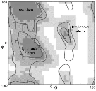
Figure 1.8 is a classic Ramachandran plot defining torsion angles.(Lovell, Davis et al. 2003)
The conformations with φ and ψ falling into dark gray regions, i.e. β-sheet and right handed
α-helix, have no steric conflict, so they are strictly allowed. If slightly shorter van der Waals
radii were used in the calculation, φ and ψ in medium gray regions are allowed as well. At
the same time, the left-handed α-helix region showed up. White regions are sterically
disallowed for almost all amino acids, because with φ and ψ in this part the distance between
atoms is smaller than the sum of their van der Waals radii, atoms collide with each other,
resulting in unstable conformations. However, glycine has no side chains, so it becomes the
only amino acid structure allowed in white regions. (Figure 1.8) With the increasing
availability of high-resolution protein structures obtained in the past few decades, refined
Ramachandran plots can be used to estimate the backbone conformation and evaluate the
quality of the structure refinement simultaneously.
Specifically, the protein helices are mainly categorized into alpha-helices, 310 helices and π-helices based on the number of residues and atoms per turn. Alpha π-helices have 3.6 residues
and 13 atoms per turn, 310 helices have 3.2 residues and 12 atoms per turn, and π-helices have 4.4 residues and 16 atoms per turn. Torsion angles phi and psi are accordingly different in
these three cases. We need to modify the values of torsion angles in structural fitting
7
1.2.2 Hydrophobicity of Amino Acid Residues
Hydrophobicity is very useful in prediction and evaluation of transmembrane helices region
of membrane proteins as well. The more positive the hydrophobicity scale, the more likely
are the amino acids to reside in the hydrophobic core of biological membrane.(Jack Kyte
1982; White 1996; Tara Hessa 2005) (Figure 1.9) kdHydrophobicity, wwHydrophobicity and
hhHydrophobicity are the hydrophobicity scales most commonly assigned to amino acid
residues. Among them, wwHydrophobicity, i.e. the Wimley-White whole residue
hydrophobicity scale, is based on transfer free energies of polypeptides directly determined
in experiments and considers not only the backbone peptide bonds but also the contribution
from side chain. It is significant in determination of the positions of amino acid residues
across the membrane.
1.2.3 Molecular Modeling using Rosetta Software Package
To get an idea about the complexity of protein folding, let us consider the backbone structure
by sequentially connecting the amino acid residues and looking for all possible torsion angles
associated with each peptide plane, assuming the value of torsion angles and are chosen
from one of the three most stable regions, i.e. the dark grey regions shown in Figure1.8. For a
small polypeptide containing only 50 amino acid residues and thus 49 peptide bonds and 98
torsion angles, in order to calculate all of its possible structures it would take 398 multiples of the time steps that are needed to find one torsion angle conformation. Therefore, the total
time to find the native structure could be even longer than the age of the universe, as
8 Molecular dynamics is commonly used in the study of protein folding using force fields to
simulate the physical movements and the interactions between atoms by solving Newton’s
equation of motion. However, in order to simulate the real dynamic processes occurred in the
object system, molecular dynamics modeling needs a large amount of computational time
even with the latest CPU. Some well-known packages, such as CHARMM (Bernard R.
Brooks 1983; Alexander D. MacKerell Jr. 2000; B. R. Brooks 2009), AMBER (Jay W.
Ponder 2003; David A. Case 2005), GROMACS (H.J.C. Berendsen 1995; David Van Der
Spoel 2005) have been well established and widely applied in research of both soluble
proteins and membrane proteins.
Early in 1961, Anfinsen (C. B. Anfinsen 1961) and coworkers had demonstrated that the
three-dimensional protein structures are completely determined by their amino acid
sequences. Starting from development of de novo prediction methodology, Rosetta has been
expanding rapidly since its first launch in May of 2004. Besides the initial de novo folding protocol, comparative modeling, protein-protein docking, protein-ligand docking, loop
modeling, protein design and enzyme design protocols etc. have been developed in the past
few years.(Baker 2000; Brian Kuhlman 2003; Jeffrey J. Gray 2003; Daniel J Mandell 2009;
James Thompson 2011) Applications such as RosettaNMR (Yang Shen 2008; Yang Shen
2009) and RosettaEPR (Stephanie J. Hirst 2011) are also developed to build protein models
from sparse experimental data. In RosettaNMR, local distance restraints are derived from
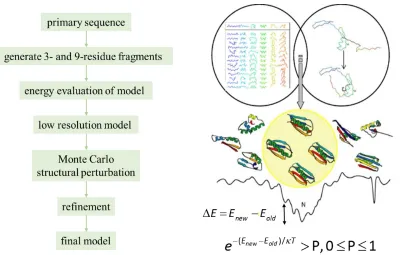
9 Combining Monte Carlo structural perturbation with energy minimization, thousands of local
minima are sampled to find a global minimum. Basically, the protocols in Rosetta can be
divided into two steps: sampling and scoring.
1.2.4 Rosetta Sampling Algorithm
Noticing the fact that the folding of local segments of a polypeptide is not dependent on the
folding of the whole protein, the Baker group has developed a molecular modeling package,
Rosetta, to predict the conformation of biological macromolecules based on the Bayesian
statistical analysis of available conformations of sequence segments in known protein
structures available in protein data bank. (Kim T. Simons 1997; Bonneau, Tsai et al. 2001;
Richard Bonneau 2002) The protein folding starts from an extended polypeptide chain. The
3-residue and 9-residue fragments with similar sequences found in the fragment library are
inserted into the protein backbone to build simulated models. Usually about 30000 9-residues
fragments and 10000 3-residue fragments are searched and combined in each model
prediction. (Carol A. Rohl 2004) Then the low-resolution energies for all the predicted
models are calculated to produce a broad range of energy minimum, and with Metropolis
Monte Carlo simulated annealing optimization algorithm the global energy minimum can be
determined. In the optimization procedure, the initial conformation is selected randomly, then
a local perturbation is conducted by modifying torsion angles or replacing a rotamer at side
chains. If the energy of the new conformation is lower than that of the old model, the new
conformation will be accepted. Otherwise, the value of e(EnewEold)/T will be calculated and
compared to a random probability P, where0 P 1 : if e(EnewEold)/T> P, the new
10 step; if e(EnewEold)/T< P, the old conformation will be kept, and a new perturbation will be
conducted. Consequently, the searching will be able to hop the local energy minima and
achieve the global energy minimum. Experimental data and constraints derived from NMR
and EPR can also assist in improving the resolution of predicted protein structure. (Philip
Bradley 2005; Kira M. S. Misura 2006; Bin Qian 2007)
1.2.5 Rosetta Scoring Function
Rosetta scoring functions, i.e. energy function, can be categorized into two major classes:
low resolution and high resolution. The former utilizes reduced atom representation and
describes side-chain with “super atoms”. This centroid-mode scoring function is mainly used
for de novo folding protocols. The high-resolution scoring function describes side-chain with
rotamers developed by Dunbrack et al (Roland L. Dunbrack Jr 1993; Karplus 1994; Roland
L. Dunbrack Jr. 1997), i.e. all-atom representation, and uses the sum of a series of weighted
energy terms as the total energy for the model. In the present project, low resolution
centroid-mode scoring function is used in de novo prediction of membrane proteins, and high
resolution all-atom scoring function is used in validation of membrane protein structures
calculated from solid state NMR experimental data.
The energy terms are physical potentials calculated by Newton’s law, van der Waals forces
as well as Coulomb’s law, and knowledge based potentials obtained statistically from the
physical characteristics of experimental protein structures available in PDB (Frances C.
Bernstein 1977; H. M. Berman 2002; Gautam Dantas 2003), including 6-12 Lennard-Jones
11 term, torsion angle preference term and an energy term based on the probability of a certain
amino acid at a given pair of phi/psi angles. (Baker 2000; Brian Kuhlman 2003)
The 6-12 Lennard-Jones potential is used to describe van der Waals interactions and
expressed by an attractive energy term Eljatr and a repulsive energy term Eljrep. (Eyal Neria
1996; Baker 2000)
12 6
2
natom natom
ij ij
ljatr ij
i j i ij ij
r r E e d d
if ij 1.12ij r
d (1.1)
10.0 11.2 natom natom
ij ljrep
i j i ij
d E r
if ij 1.12ij r
d (1.2)
wherei and j are indices of different atoms, dij is the distance between the two atoms, rij is the
sum of the van der Waals radii, and eij is the square root of the product of the well depths by
adapting the CHARMM19 parameter set via using 5% shorter van der Waals radii. When dij
equals rij, the value of the attractive energy is the sum of -eij. When the distance between two
atoms is 0 Å, the repulsive energy reaches its maximum 10.0 kcal/mol.
The solvation potential Esolv is derived from semi-empirical implicit solvent model
parameterized with experimental data, which was initially promoted by Lazaridis and
Karplus. (Themis Lazaridis 1999) Burial of polar atoms is also penalized as part of the
solvation potential. Esolv penalizes surface exposure of hydrophobic residues and favors
exposure of hydrophilic residues.
2 2
2 2
2 2
exp( ) exp( )
4 4 free free natom natom j ref i
solv i ij j ji i
i j i i ij j ij
G G
E G d V d V
r r
12
dij and rij have the same definition as mentioned above. Grefis the solvation free energy of
the fully solvated atom. λij is a correlation length, and V is the atomic volume.
The electrostatic interactions are demonstrated by residue pair potential Epair (Kim T. Simons
1999), and hydrogen bonding potential Ehbond. The residue pair potential is knowledge based
and obtained from the probability of a pair of polar residues found in the vicinity of each
other in PDB database.
( , | , , )
( | , ) ( | , )
nres nres
i j ij i j
pair
i j i i ij i J ij J P aa aa d env env E
P aa d env P aa d env
(1.4)In Eq. (1.4), i and j are indices for different amino acid residues, P aa d env( i| ,ij i) is the
probability of finding amino acid type aai within the distance dij in local environment type i,
and P aa d env( J| ,ij J) is the probability of finding amino acid type aaj within the distance dij in
local environment type j.
The hydrogen bonding potential is orientation-dependent and consists of long-range and
short-range items, i.e. hbond_lr_bb, hbond_sr_bb, hbond_bb_sc and hbond_sc (D Benjamin
Gordon 1999; William J. Wedemeyer 2003).
12 10
5 ij 6 ij ( )
hbond
ij ij
r r
E F q
d d (1.5)
dij is the distance between acceptor and donor of the hydrogen bond, and rijis the optimal
hydrogen bonding distance. F(q) is the angular dependence of the hydrogen bond calculated from vector-angle potential, vector-tensor potential and vector-displacement potentials
13 Rotamer self-energy Erot is calculated from the probability of finding a certain rotamer at a
given pair of phi/psi torsion angles in protein data bank, and is based on Dunbrack rotamer
library. (Roland L. Dunbrack Jr 1993; Karplus 1994; Roland L. Dunbrack Jr. 1997)
ln( ( ( )| ( ), ( )) residue
rot i
E
prob rot i phi i psi i (1.6)The torsion potential Erama is based on the Ramachandran torsion angle preferences and is
calculated from the probability of finding a certain amino acid in a secondary protein
structure at a given pair of phi/psi torsion angles in protein data bank.(G.N. Ramachandran
1963; William J. Wedemeyer 2003; Carol A. Rohl 2004)
ln[ ( ( ), ( )| , )] residue
rama i i
i
E
prob phi i psi i aa ss (1.7), where aa = amino acid type and ss = secondary structure type.
1.2.6 Assessment of Model Quality
The accuracy of predicted models are evaluated mainly by three factors, i.e. RMSD,
GDTMM and MaxSub. RMSD is the root mean square deviation of the simulated structure to
the native structure if a crystal structure is available. Otherwise, the lowest energy structure is
usually used as the baseline to calculate RMSD. GDTMM (James Thompson 2011) measures
the superposition between the simulated structures and the native structure, and with a given
distance cutoff, the closer is GDTMM to 1.0, the more similar is the predicted model to the
native structure. MaxSub (Naomi Siew 2000) describes the largest subset of C atoms of a
simulated structure that superimpose well over the native structure with a given RMSD
14
1.3 Solid-State NMR Studies of Membrane Proteins 1.3.1 Basic Principles of NMR
In NMR spectroscopy, Nuclear Overhauser Effect (NOE), chemical shifts, J-coupling,
dipole-dipole coupling and quadrupolar couplings are the nuclear spin interactions normally
utilized for structure determination. NOE (Overhauser 1953; Kaiser 1963) describes the
magnetization transfer between dipole-dipole coupled nuclear spins and mainly provides
information about distance between these nuclei pairs. J-couplings (Maxwell 1952) describe
the inter-nuclear spin interaction through chemical bonds and provide both distance and
angular information. Both NOE’s and J-couplings are usually probed in solution NMR
spectroscopy. By contrast, chemical shift anisotropy, dipolar couplings and quadrupolar
couplings are all anisotropic in solid samples, and, therefore, represent a useful source of
information for membrane protein structure determination from solid-state NMR
spectroscopy. Chemical shift anisotropy demonstrates the orientation dependence of the
chemical shift and arises from that fact that the charge distribution on a nuclei is not
spherically symmetric. The orientation of the atoms affect the orientation of the electron
cloud over the nuclei, and thus affect the chemical shielding. Dipolar couplings, different
from J-couplings which describe through-space dipole-dipole interaction, indicate direct
interactions between dipole-dipole coupled nuclear spins. Distances and bond orientations
between the nuclei can be obtained directly from NMR spectroscopic data. Quadrupolar
couplings (Lucio Frydman 1995) appear in nuclei with a spin larger than ½ and depend on
the electric field gradient. Both dynamic and orientational information can be obtained in
15 In most NMR experiments, backbone atoms (amide nitrogen, alpha carbon and carbonyl
carbon) in polypeptide chains are isotopically labeled for frequency measurement.
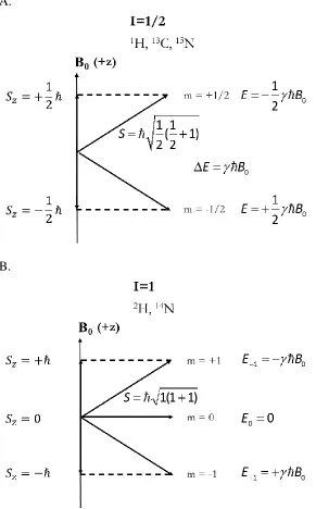
Nuclear magnetism is originated from nuclear spin angular momentum, I, which is an
intrinsic property of nucleus. When I=0, usually found in atoms with both even mass number and even atomic number like 126C, the nuclei have no magnetic moment and no NMR signal
can be detected. Both 15N and 13C used to label a protein sample in solid state NMR
experiments have a nuclear spin with I equal to ½. Quadrupolar couplings can be measured in nuclei with I > ½ like 14N.
The magnetic moment can be expressed by the product of nuclear spin angular momentum
S and gyromagnetic ratio , i.e. S. If we represent the spin angular momentum with S,
then the square of its observable value is given by:
1
2I I
2
S (1.8)
where I stands for the angular momentum quantum number and ħ is the reduced Planck’s constant.
For a static magnetic field B0, its orientation is defined along the z-axis, and the projection of the angular momentum S on the z axis can be described by Sz=mħ, where m is the magnetic quantum number, and m ranges from I, I-1,….to –(I-1), -I. Then the z-component of the magnetic moment z=mħ. Therefore, in the magnetic field B0, the energy of a nuclear spin state can be calculated using E = -zB0 = -mħB0 , and the difference of energy between two
16 nucleus with spin I=1, the energy difference is ΔE=2ħB0. The angular momentum operators are also used in the calculation of Wigner rotation matrix in structural fitting. (see Eq. (2.4))
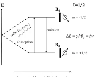
The ratio of the populations of two spin states, N(- ½ ) and N(+ ½ ) at temperature T is related to the Boltzmann constant κ and the energy difference between the two states.
/ /
( 1/2)/ ( 1/2) /
E T h T
N N N Ne e (1.9) By absorbing energy from radio frequency, N- will increase and N+ will decrease, thus the ratio N- / N+ will increase. Based on this phenomenon, the sensitivity of sparse nuclear spins in NMR experiments, such as 15N and 13C, can be increased via their interaction with a
collection of abundant spins like 1H. The abundant spin system is prepared under an assigned low temperature, then the sparse spin system is brought into the cold system of the abundant
spins via thermal contact. As the energy is transferred from the sparse spin system to the
abundant spin system, the population between the higher energy and lower energy spin states
will increase. Therefore, the sensitivity of the NMR experiments can be improved.
The resonant condition for absorbing radio frequency radiation is given by: E=h, B0/2π. Consequently, the resonance frequencies observed for different nuclei are proportional to
their corresponding gyromagnetic ratio.
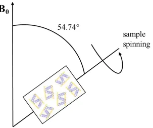
1.3.2 Magic Angle Spinning NMR
In magic angle spinning (MAS) solid-state NMR, the orientations of the protein molecules
immobilized in randomly oriented lipid bilayers with respect to the external magnetic field is
averaged out by the sample rotation about 54.74°, i.e. the magic angle. By mechanically
spinning membrane protein samples at the magic angle at a high frequency of 1-70 kHz,
17 anisotropy is averaged to the isotropic component of the CSA tensor, and the quadrupolar
coupling is partially averaged to a residual second moment. This results in a high resolution
spectrum with narrower lines containing only isotropic shifts and J couplings, such as those
obtained from solution NMR, thus providing distance and torsion angle information. Figure
1.13 shows a schematic diagram of a typical MAS experiment. (E. R. ANDREW 1958; Lowe
1959; Andrew 1981; Jaume Torres 2003)
1.3.3 Oriented Solid-State NMR
In oriented solid state NMR, bicelles and lipid bilayers, which encompass the membrane
protein samples and serve as a native-like environment (Isabelle Marcotte 2005), are
magnetically aligned either perpendicular or parallel (with the addition of lanthanide ions) to
the external magnetic field. (Figure 1.14) Orientation-dependent chemical shift anisotropy
and heteronuclear spin-spin coupling are the conformational constraints used to predict
membrane protein structures. Many experimental methods, such as MREV8 (W-K. Rhim
1973), TMREV (M. Hohwy 2000), PISEMA (Wu, Ramamoorthy et al. 1994) and SAMMY
(Alexander A Nevzorov 2003), have been developed to measure the dipolar nuclear spin
interactions since the establishment of solid-state NMR spectroscopy. These pulse sequences
belong to the so-called class of high-resolution separated-local field experiments. For
instance, PISEMA (Polarization Inversion Spin Exchange at Magic Angle) is a useful tool to
analyze the conformations of helical membrane proteins, while recent publications
demonstrated that β-barrel fractions in membrane proteins can be resolved as well. (Ana
Carolina Zeri 2003; Nevzorov and Opella 2003; David S. Thiriot 2004; De Angelis, Howell
18 PISEMA correlates 15N chemical shift anisotropy and 1H-15N dipolar coupling for uniformly or selectively 15N labeled proteins highly aligned in the magnetic field. Mathematically, the
observables in a PISEMA experiment can be described as
0π B = σ,ν
(1.10)
, where σ is chemical shift tensor and ν is dipolar splitting tensor.(Denny, Wang et al. 2001)
The chemical shift tensor σ is asymmetric, and its principal axis frame (PAF) is represented
as = σ ,σ11 22,σ33
PAF . σ11, σ22, σ33 are the corresponding principal values and satisfy σ11<=
σ22<= σ33. The value of chemical shift tensor is given by
2 2 2
11 0 11 22 0 22 33 0 33
σ = σ B σ + σ B σ + σ B σ
(1.11).
The dipolar splitting tensor ν is traceless and axially symmetric with a unique rotation axis
along the direction of covalent bond NH and can be represented as
2 ||
0 ν
ν = 3 B u -1 2
(1.12)
, where ν|| is the value of dipolar splitting tensor when B0 u
. If the coordinates of unit
vector of B0 in PAF are (x, y, z), tensor σ and ν can be expressed by
2 2 2
11 22 33
σ = σ x +σ y +σ z
(1.13)and
2
|| ν
ν = 3 cos sin x + sin sin y + cos z -1
19 The periodicity in the orientation of each peptide plane in an ideal helix is reflected into a
characteristic PISEMA pattern, i.e. the PISA (Polar Index Slant Angle) wheel. By analyzing
the PISA wheels, one can assign the resonances sequentially to the corresponding amino acid
residues in the polypeptide chain and determine the orientation of alpha helices and beta
sheets with respect to the external magnetic field. (J. Wang 2000; Marassi and Opella 2002;
Nevzorov and Opella 2003; A. Ramamoorthy 2004) As the slant angle τ relative to the
magnetic field increases, the PISA wheel moves from top left to bottom right while the radius
first expands and then reduces in its size. (Figure 1.15)
In the PISEMA coordinates, the formulation of the dipolar coupling and chemical shift
anisotropy are both in a quadratic form, so the values with equivalent magnitudes but
opposite signs can all satisfy the equation, leading to a large number of possible orientational
solutions. The orientations of the peptide planes are four- to eight-fold degenerate owing to
the quadratic nature of the relevant NMR interactions, as well as to the fact that only the
absolute values of the dipolar coupling could be determined experimentally. If
multidimensional spectra including 13Cα chemical shift, 13Cα-1Hα dipolar coupling and even 13
Cβ-1Hα dipolar coupling are available, these degeneracies could be removed and the conformation of side chains can be unambiguously resolved. (Nevzorov and Opella 2006)
Ramachandran maps could also be used as a means of removing these degeneracies by
constricting only those peptide orientations that result in plausible torsion angles φ and ψ as
20
1.3.4 Structural Fitting using PISEMA
Structural fitting of the PISEMA spectra has proved to be a useful method to determine the
membrane protein structure, particularly irregular structures like kinks, twists and bends,
from the frequencies measured in solid-state NMR spectra. (Thomas Vosegaard 2002;
Bertram, Asbury et al. 2003; Nevzorov and Opella 2003; J. R. Quine 2004) The programs
SIMPSON and SIMMOL (Mads Bak 2002) have been developed by Nielsen and coworkers
since 2000, while CNS-SS02, a pubic software package developed from CNS
(Crystallography & NMR System) software (A. T. Brünger 1998), is also a common tool
used in structural fitting. Around 2003, a Monte Carlo simulation algorithm implemented in
MATLAB was established by Nevzorov and Opella for structural fitting with partial or
incomplete resonance assignment of the PISEMA spectra. (Nevzorov and Opella 2003; Anna
A. De Angelis 2004; David S. Thiriot 2004; De Angelis, Howell et al. 2006; Sang Ho Park
2006) Nevzorov and Opella have applied this algorithm to the experimental data of an
18-residue ideal α-helix containing only alanines, a 16-18-residue single α-helical transmembrane
domain of the channel-forming peptide from the acetylcholine receptor (AchR M2), and a
25-residue transmembrane α-helix of the fd-coat protein to compare the structural fits under
different conditions, such as different variation ranges in the torsion angles and incomplete or
partial assignment of the spectra. For the ideal α-helix fragment, there is no obvious
difference between the structural fits for the ±5° and ±10° variations in the torsion angles φ
and ψ. For the α-helical transmembrane domain in AchR M2, the structural fit is virtually
unique when the variation region for the torsion angles is ±5°. But when the variation region
21 RMSD (root mean square deviation) of less than 2Å. In addition, if additional resonances of
some specific types of residues are available, the structural fit could be more accurate
(RMSD < 1.6 Å) even with a relatively large variation (±10°) in the torsion angles. For the
transmembrane α-helices of the fd-coat protein, Nevzorov and Opella also compared the
structural fits with and without specific resonance assignment of some types of residues, and
concluded that additional resonance assignment of some residues can help achieve a
convergent set of solutions with higher accuracy and precision.
1.3.5 Analytical Framework for Solid-State NMR Observables in Torsion-Angle Space
To implement the structural fitting of multidimensional solid-state NMR spectra of aligned
samples, it is necessary to establish an effective analytical framework to transform the data
from solid-state NMR spectra into the protein structures.
In Cartesian coordinate system, a point in space can be represented by a row vector r:
r
x
y z
(1.15)Here, x, y, and z are the Cartesian coordinates of the point. Assuming the Cartesian basis as a
standard right-handed coordinate system and the rotation counterclockwise, the basic rotation
matrices in three dimension space are:
10 cos0 sin0 0 sin cos xR
cos0 01 sin0 sin 0 cos y R
cossin cossin 000 0 1
z R (1.16)
To rotate an old coordinate system into a new one with coordinates of the same vector, we
22
' '
cos cos cos sin sin cos cos sin sin cos cos sin
sin cos cos cos sin sin cos sin
cos sin 0 cos 0 sin cos sin 0
sin cos 0 0 1 0 sin cos 0
0 0 1 sin 0 cos 0 0 1
tot Z Y Z
R R R R
cos cos sin sin
sin cos sin sin cos
(1.17)
So the coordinates of the vector in the new system can be expressed by:
x
'
y
'
z
'
x
y z R
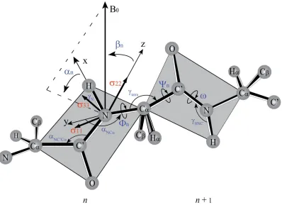
tot (1.18)In this analytical framework, a molecular frame associated with the peptide plane is
introduced, the x-axis is chosen along the NH bond, and z-axis is perpendicular to the plane
containing NH and NC’ bonds. The orientation of applied magnetic field relative to the
molecular frame of the nth peptide plane is described by angles αn and βn. Hence, 15N chemical shift anisotropy and 1H-15N dipolar coupling can be written as:
15 2 2 2 2 2
11 22 33
( ) sin sin cos sin cos
N (1.19)
2 21 15 3sin cos 1 2
H N (1.20)Aiming at calculating the protein structure directly from its solid-state NMR spectrum in an
ab initio fashion, we should determine the minimum number of experimental angular
constraints that are necessary to determine a complete atomic-resolution structure of a
protein.
However, in solid-state NMR, both spatial and angular constraints are the observables in the
measurement, so a coordinate system, which is called rank-1 irreducible spherical basis,
23 project, therefore, we choose this basis to relate the protein structure to its multidimensional
solid-state NMR spectrum.
Since the bond lengths
x
2
y
2z
2 remain constant, the spherical basis is obtained from theCartesian basis by the transformation matrix T:
1 1
0
2 2
0
2 2 2 2
0 1 0
sin sin cos
2 2
i i
i i x iy x iy
x y z z
r e e
1 1 0 2 2 0 2 2
0 1 0
i i T (1.21)
Consequently, the rotation matrix is transformed into the so-called “Rank-1 Wigner Rotation
Matrix” (Arfken 1985):
, ,
1 cos sin 1 cos
2 2 2
sin sin
cos
2 2
1 cos sin 1 cos
2 2 2
tot
i i i i i
i i
i i i i i
T R T
e e e e e
e e
e e e e e
D
(1.22)
In this irreducible spherical basis, all the frequencies obtained in the experiment can be
rewritten in a unified manner as a much more compact quadratic form.
=Y
,
D
MP MD1
MP Y
,
24 Here, Wigner rotation matrix D(ΩMP) describes the transformation from the molecular frame to the principal axis system of each tensor. The superscript “+” denotes the Hermitian
conjugate. The row vector of unnormalized spherical harmonics Y(β, α) is given by the
following formulation:
sin sin( cos )
2 2
,
i i
e e
Y (1.24)
In Eq. (1.23), M is the corresponding interaction matrix. For chemical shift anisotropy, M is
described by the principal components σ11, σ22, and σ33, given that σ33> σ22> σ11:
11 22 22 11
33
22 11 11 22
0 2 2 0 0 0 2 2
M
(1.25)For dipolar couplings, M is expressed by the product of the dipolar coupling constant and a
single diagonal matrix:
1 / 2 0 0
0 1 0
0 0 1 / 2
M
(1.26)The rotation of the subsequent peptide planes is achieved by the so-called propagator matrix.
Mathematically, the propagator matrix P(Φn, Ψn) given by the product of two rank-1 Wigner
25 calculated via operating the propagator matrix on the spherical harmonics of the n’th peptide plane.
(
n,
n)
NC,
n,
tetra
0,
n
,
C CP
D
D
(1.27)
1, 1
,
,
n n n n P n n
Y Y (1.28)
In the propagator matrix, the first Euler angle in the first Wigner matrix is the angle between
the y-axis of the molecular frame and the N-Cα bond of the nth peptide plane, NC =151.8º; the third Euler angle in the first Wigner matrix is the tetrahedral angle, γideal=109.47º, but in real protein typically γ=110º-112º; the third Euler angle in the second Wigner matrix is the
angle between the Cα-C bond and the y-axis of the molecular frame of the (n+1)th peptide
plane, C C =34.9º. These numerical values of Euler angles are assumed to be constants for
each peptide residue of the structure, so as long as the torsion angles Φn and Ψn are
determined, the backbone conformation of the complete protein can be constructed residue
by residue. The peptide plane can be also described by three directional vectors μ1, μ2 and μ3 with formulation expressed by Eq. (1.29) in the irreducible spherical basis.
2 2
k k k k
k k
x iy x iy
z (1.29)
Here, μ1 denotes the directional vector ending at carbonyl carbon, μ2 ending at nitrogen and μ3 ending at the α-carbon. (xk, yk, zk) are the vector coordinates measured relative to the
26 peptide plane relative to the laboratory frame can be calculated using Eq. (1.30), while Eq.
(1.31) works for the succeeding residues.
1
11 1
0, ,
T
k kD (1.30)
1 1
(
,
,
)
n T
n T
k k
P
n n n (1.31)1.4 Prediction of Helical Membrane Proteins Structures using Rosetta
1.4.1 De Novo Prediction using Membrane Ab Initio in Rosetta
Many research groups analyzed the available alpha-helical membrane protein structures
statistically and summarized the amino acid environmental preferences within hydrophobic,
amphiphilic (interface) and polar layers of the membrane. Based on this information,
Yarov-Yarovoy et al. have adapted original Rosetta de novo structure prediction method to predict
the helical transmembrane protein structures. (Vladimir Yarov-Yarovoy 2006) In the tests on
12 membrane proteins with known structure, such as rhodopsin, V-type Na+-ATPase,
bacteriorhodopsin and lactose permease transporter, 51-145 residues were predicted with
RMSD less than 4Å to the corresponding native structure.
The energy of predicted structure is calculated by Eq.1.32 (Vladimir Yarov-Yarovoy 2006),
considering residue-environment interaction, residue-residue interaction, steric overlapping,
packing density of membrane proteins and strand pairings. The energy maximizes exposure
of hydrophobic residues within the membrane and minimizes hydrophobic exposure outside
the membrane. The membrane protein database is constituted by 28 helical transmembrane
protein structures in PDB.
27 First of all, the amino acid sequence is used to generate three- and nine-residue peptide
fragments on Robetta server (http://robetta.bakerlab.org/), which is more convenient and
accurate than the traditional PSIPRED (Jones 1999), JUFO (Meiler 2003) and SAM-T99
(Kevin Karplus 2001).
Different from de novo prediction for soluble protein structures, besides the FASTA primary
sequence file, three-residue and nine-residue peptide fragments files, transmembrane
topology prediction file and lipophilicity prediction file are also necessary and significant in
membrane ab initio simulation.
Transmembrane region is predicted on OCTOPUS server (http://octopus.cbr.su.se/) with
primary sequence in FASTA format as input file, and expressed by i, o and M in the output file. (Elofsson 2008) M, standing for membrane, is assigned to residues < 13 Å from the membrane center. i and o are assigned to residues in loop regions, which is 13-23 Å from the membrane center. inside (i) or outside (o) depends on the side of the membrane they reside on. Figure 1.17 demonstrates the definition of membrane and the allowed region for
transmembrane hairpins by OCTOPUS. Then the transmembrane topology prediction file,
i.e. SPAN file, is generated using the OCTOPUS file. The number of transmembrane helices
and the start and end residue numbers of each single predicted transmembrane helix are
shown in the SPAN file. Finally, with sequence file and SPAN file as input, the predicted
lipophilicity file, i.e. LIPS4 file, is produced.
The membrane ab initio protocol sets the initial membrane center as the center of the mass of
the protein and the membrane normal unit vectors as the average direction of all the helices