Boosting Data Center Performance
Through Non-Uniform Power Allocation
∗Mark E. Femal Vincent W. Freeh
Department of Computer Science
North Carolina State University
{mefemal,vwfreeh}@ncsu.edu
Abstract
Data center power management is evolving fromad hocmethods based on maximum node power usage to systematic methods that employ power-scalable compo-nents. In addition, it is possible to exploit the power and throughput relationship to increase the total work per-formed and safely overprovision the rack space while staying below an aggregate power limit. This research describes a general framework for boosting throughput at a local level while load-balancing the available ag-gregate power under a set of operating constraints. Our solution is useful for those data centers that cannot ex-pand the number of power circuits or seek effective us-age of their available power budget due to unplanned power fluctuations. The framework is particularly well suited for environments with a heterogeneous workload and hence, a non-uniform power allocation requirement. Based on a representative workload for a two minute pe-riod, this paper shows a non-uniform power allocation scheme increases throughput by over 16% versus a uni-form power allocation mechanism.
1. Introduction
The tremendous increase in computer performance has come with an even greater increase in power us-age. As a result, power consumption is a primary con-cern. According to Eric Schmidt, CEO of Google, what matters most to Google “is not speed but power—low power, because data centers can consume as much elec-tricity as a city” [23]. This does not imply speed is not important for computing centers, but more and more
∗ This research was supported in part by an IBM UPP award.
sites find themselves operating with a power constraint due to increased performance. Such a limit might ex-ist due to either a limited power supply or heat dissipa-tion and removal capacity. In addidissipa-tion, reducing the me-tered energy or associated power and cooling infrastruc-ture costs might be a high priority. Regardless of the
rea-son, a power constraint is aperformance-limitingfactor.
Many data center operators utilize manually intensive methods that are prone to error to avoid exceeding power circuit capacity. A conservative power management ap-proach is to ensure the maximum power consumption of all nodes never exceeds the power circuit capacity based
on a global limit,G. In such a cluster, this conservative
approach first defines the maximum power a single node
might consume,Lmax. Data center personnel then
sub-sequently deploy as many similarly configured nodes as
possible under the global limit (i.e.,n = b G
Lmaxc). In
general, the maximum power consumption of a node is much more than the average power consumption. There-fore, the conservative approach under utilizes power and
artificially lowers the limit ton · Lavg < G.
One can overprovision by deploying m > n
nodes; however, unsupervised methods risk exceed-ing the global limit. Exceedexceed-ing the limit will likely trig-ger a reaction that reduces power consumption. This reaction could be as drastic as a circuit breaker trip-ping or less severe as to require other manual in-tervention in the recovery process. Both of these situations are undesirable, but are typically the nor-mal plan of action in many environments. Therefore, we have developed a mechanism to facilitate safe over-provisioning that automatically controls power usage while avoiding excessive, long-term power consump-tion [10].
This paper presents improvements to our prior work, as well as a novel, dynamic algorithm to manage power
This extension performspower load balancingto effi-ciently utilize available power given the circuit capacity. Because power consumption is irregular, as is task de-mand, one needs a dynamic and adaptive solution.
There are two autonomic managers within our frame-work. One manages a node’s target power consumption, beneath a local power limit. The other component as-signs this local power limit based on aggregate cluster workload and the global power circuit capacity. For sim-plicity, we confine the remaining discussion to manag-ing instantaneous power. Because energy is power inte-grated over time, managing energy is merely managing average power. Similarly, heat generation is a function of energy consumption and can be addressed in a simi-lar fashion.
This paper makes three contributions. First, it intro-duces the idea of power load balancing and motivates its necessity. Second, it establishes the need for and creates a global power allocation mechanism to assign power in order to achieve efficient application throughput. Fi-nally, this paper presents refinements to our local power controller to ensure a node is assigned a local power limit indicative of its workload contribution in a clus-ter.
The remainder of the paper is organized as follows. The next section presents related work. Section 3 de-scribes the overall model and Section 4 discusses the im-plementation. Section 5 presents our results and we con-clude with a summary and discussion of future work.
2. Related Work
The case for a closer relationship between the op-erating system and power management is explored in [32, 8]. Flinn and Satyanarayanan [12, 13] show that co-ordination with applications can yield significant power savings. Dynamic voltage scaling (changing both fre-quency and voltage) to reduce power consumption is ex-plored in [11, 15, 26, 29, 19]. In [21], forecast meth-ods are used on a single node to minimize power con-sumption. Unlike this work, we choose to automatically change the forecast model based on past prediction ef-ficiency as well as increase throughput subject to power limits.
Power management in commercial servers is impor-tant for web servers [4, 22]. Much of this work relies on load balancers to distribute work. An investigation of load balancing was done in [27, 28] to turn cluster nodes on or off based on load. Additional research has
also been done by Elnozahy et al. [9] for developing
mechanisms for energy-efficient clusters using
combi-nations of IVS, CVS, and VOVO policies. Although the VOVO policy is not considered in our initial implemen-tation, its importance is less significant with heteroge-nous workloads. In [7], an economic approach is chosen to determine the minimal number of servers required to handle the load. Unlike [7] we favor a decentralized ap-proach and seek to increase throughput. In [31], Sharma
et al.applies real-time techniques to web servers in or-der to conserve energy and maintain QoS. Managing to service metrics is an instance of a target power alloca-tion mechanism in our model once a power limit is de-fined.
The approach of estimating power consumption us-ing performance counters is taken in [2, 20, 14] and is complementary to our notion of target power as-signment. We are investigating the usage of program counters as a means of identifying intra-node perfor-mance bottlenecks. Identifying such occurrences may provide the opportunity for an additional power reduc-tion in other power-scalable components with no loss in throughput.
In server farms, disk energy consumption is also im-portant. One study of four energy conservation schemes concludes by stating that reducing spindle speed is the only option for clusters [6]. DRPM is a scheme to mod-ulate the speed of the disk dynamically to save energy [16, 17] rather than stopping disk rotation. We plan to investigate this approach in future efforts.
While analyzing energy efficiency and operat-ing points in [25], it is found that the most energy ef-ficient gear is not always the lower performance point.
All past power research for server clusters (i.e., as in
[5, 7, 9]) has focused on uniform workload distribu-tion with migratable loads. This work has a contribu-tion towards policy development in the management of power limits, but not all environments have the lux-ury of migrating work due to expense, complexity, or other factors.
3. Non-Uniform Power Allocation
With more than one node, power can be allocated to nodes non-uniformly. A uniform allocation is best only when the workload (and application performance) is identical on each node. There are four primary goals in global power allocation. The first goal ensures to-tal power consumption is below the global limit and
available power is equitably distributed (e.g., no node
pro-vided a degredation in the power supply occurs (i.e., de-creases due to partial power loss). The final power allo-cation goal ensures the solution is easy to deploy, main-tain, and operate transparently with minimal tuning. To this end, a distributed algorithm is used to learn and react to cluster modifications automatically. No central point of failure exists and the per-node computational re-quirement is minimal. In addition, all current power con-sumption and minimum power requirements are avail-able to administrators. This information offers a site the ability to identify power deficiencies and facilitates safe overprovisioning.
The global power allocation model dynamically and non-uniformly allocates power among nodes to increase aggregate performance given irregular workloads. To make this work in practice, time must be divided into
discrete processing intervals. At timet, the data for past
intervals is evaluated for the next interval. From this in-formation, a forecast of expected work is calculated on each node. Given this knowledge, a prediction is made of expected need for each node and is then used in the next reallocation. Each node’s expected need is weighed in conjunction with the expected aggregate workload. There are two power limits in our framework. The first exists to limit local node power consumption and is a calculated quantity based on cluster constraints. The sec-ond is the global limit and is assigned to a cluster based on circuit capacity. Each of these limits will now be cov-ered in greater detail.
3.1. Local Power Limit
The calculated, locally assigned power limit,L, for
each participant in the network is regarded as a mutual
decision based on all node and global constraints (e.g.,
power reserve). Using its assigned local limit, a node is responsible for suballocation of power at a fine-grain level. To ensure local minimum service constraints are
met,Lmin represents the power needed to guarantee a
minimum service level. In addition,Lmaxis the
maxi-mum quantity of power a node uses due to technical
lim-itations (i.e., maximum consumption possible given
con-nected devices).
At the node architectural level, each device in a node has an interface to relay or provide information related to power draw, performance states, as well as minimum and maximum power required to function. Although el-ements of this are available in laptop systems using the ACPI specification [18], future development of con-sistent interfaces to hardware should promote similar
hardware sensors and functionality for servers using the same methods.
Each node manages average power consumption
ac-cording to a target,T (a value less thanL). Ideally, this
average is close to the assigned local limit, but a burst
term represented by B is used to reflect an additional
quantity above T needed to properly manage average
power consumption (there is a delay in reacting to power usage). The power consumption target is adjusted lo-cally as needed and no restrictions are imposed in the
general model (i.e., this concept allows an energy
con-servation or other model to be employed). In general, the local node power relationship is governed by:
Lmin≤T+B ≤L≤Lmax.
Intuitively, based on the magnitude ofL−(T+B)
a node signals to other nodes it has either a surplus or deficit. If this value is zero, a node is using its full al-location. If less than zero, a node has a power surplus. However, these conditions are not the sole means of re-allocation. Additional consideration is needed when de-mand exceeds supply and this is discussed in the next section.
3.2. Global Power Limit
The global power limit itself is known and quantifi-able based on circuit capacity. The allocation problem
is to calculateLfor each nodeisuch thatPni=1Li ≤
G. Furthermore, given knowledge of the workload
de-mand for each node, increase the efficiency in allocat-ing available power for each node given the contribu-tion of its work with respect to the aggregate demand,
Wtotal =
Pn
i=1Wi(Li). This problem is not solvable
because work performed for a given power limit changes dynamically and is not known a priori. Therefore, we first allocate as much of the available power as
possi-ble to keepG−Pni=1Lismall. Second, an estimate is
performed for the work contribution of each node in the next interval. This estimate ensures nodes with greater need have a higher priority. Finally, a reassignment of
all node local power limits is done fort+ 1.
Based on the estimate of aggregate global power
de-mand, if it is less thanGthe predicted aggregate power
power is needed than available, nodes receive an addi-tional allocation of power.
3.2.1. Preconditions. In order for the global allocation model to function, the following preconditions must be satisfied. First, a mechanism is required to manipulate hardware power consumption. In our current framework, this is accomplished using DVS. Second, a means of controlling power locally at each node must exist. This condition is met using a software component discussed in Section 4. Third, a system to forecast and track work-load on all nodes must exist. In addition, an estimation of the expected change of workload for each node must be made. Finally, any available power must be allocated to ensure the global limit is not exceeded, yet nodes re-ceive an appropriate value of additional power indica-tive of demand. The next two sections discuss the latter two requirements in greater detail.
3.2.2. Forecasting Workload. Given the unique
char-acteristics of power and throughput that exist in a clus-ter environment, the general trend of work completed,
Waverage, is determined based on short-term historical
demand. Using this same information, a predicted value
of demand,Wpredicted, is calculated and utilized to
fore-cast demand for the next interval. Given current node power need, an approximation is now possible for the next interval using:
A= (T +B)·Wpredicted
Waverage
The value A is bounded by several technical
con-straints. First, node power consumption cannot exceed
Lmax. In addition, a fundamental (if a node is to make
any progress) or explicit service constraint establishes a
power limit lower boundary,Lmin. In instances where
G≥Pni=1Ai, all node limits can be assigned
success-fully with no node receiving less than its desired power limit. However, if this condition does not hold, some nodes lose desired power as a result of successive itera-tions of the algorithm. This node power loss depends on its power need with respect to all nodes. Any node re-ceiving less power experiences increased local demand if its need increases faster with respect to other nodes in future intervals. This, in turn, subsequently causes addi-tional local limit increases as the global power alloca-tion method balances aggregate power based on demand throughout the whole cluster.
3.2.3. Additional Node Power. If available power is
denoted asp, then
p=G−
n
X
i=1 Ai.
Withpknown, a node specific additional power
al-location,S, is found based on work contribution,c =
Wpredicted
Wtotal . Thus,S = p · cand this value is added to
the initial approximationA. In addition,Sis bounded by
an administrative limit to prevent excessive allocation.
Intuitively,S is determined from the fractional amount
of total available power after meeting all power need
(i.e., Pn
i=1ci = 1). To further illustrate the
determi-nation of per nodeS values, consider an environment
with two cluster nodes, an available power quantity of 20 watts, and an administrative threshold of 15 watts. If each were equally contributing to aggregate workload,
the resultant per nodeS values are 10. However, if one
node is idle and its contribution is zero while the other node remains busy, the busy node receives 15 watts and the other receives none. This example is simplistic
be-cause from an implementation standpoint,Wpredictedis
restricted to nonzero values. This is to avoid dividing by zero in a completely idle environment as well as ensur-ing a minimum additional allocation is given to ensure
short-term, upward mobility forT in the next interval.
3.3. Global Allocation Solution
The need to maximize the total power used in the cluster given the current and forecasted workload under a set of constraints is actualized as a Linear Program-ming (LP) solution. This is a multi-step process and is informally defined as follows:
1. Based on the broadcast data of all nodes, calcu-late the aggregate workload for the entire cluster,
Wtotal.
2. For each node, determine its contribution,c, to
ag-gregate workload. Changes inc will reflect a gain
or loss of power from the prior interval.
3. Next, calculate the local power limit subject to all
nodeLmin,Lmax,BandTvalues.
4. For each local power limit, bound it according to
its uniqueAvalue. This value accounts for all
clus-ter demand and provides additional power to a node if needed.
5. Finally, ensure a sufficient reserve,R, is kept and
maximize:
Pn i=1Li
subject to:
Li≥Lmini Li≤Lmaxi Li≤Ai+Si
Pn
i=1Li≤G−R
Figure 1. LP model to assignLi∀i∈[1, n].
The informal steps outlined above are translated into the LP model shown in Figure 1. It is important to
rec-ognize this model is infeasible ifPn
i=1Lmini > G. One
policy to handle this occurrence is to perform a con-trolled shutdown of all or some nodes based on quality of service constraints, minimizing lost revenue, or some other measure. The current implementation does not ad-dress such an instance.
The LP objective function solution is the current total power allocation. In addition, the amount of power after allocations are made and the minimum power needed to
meet all node constraints is determined, Pn
i=1Lmini.
However, the critical outputs are all node local power limits for the next time interval. Each node determines its local limit by saving its offset within the objective function as the model is built at runtime. It is important
to notice thatAaccounts for the relative power need for
each node (either surplus or deficit). Thus, each node
in-directly decreases or increasesLby adjustingTorB. In
addition, the upwards pressure of bothWpredicted and
the administratively assigned upper threshold set forS
provide additional power to nodes.
Given the model in Figure 1, a linear program-ming solver [3] calculates the outputs using the simplex method. All values are considered to be real, con-tinuous values within their respective bounds. The complete model is built dynamically using current
clus-ter data. Rather than add additional constraints forLmin
andLmax, lower and upper variable bounds on L are
used to limit the number of true constraints. This re-duces the internal model size and solves the problem more efficiently. There is no technical limit to the
num-ber of constraints (i.e., only one additional solver
con-straint is needed for each node) and a timeout is used to generate suboptimal solutions.
4. Implementation
Two per-node autonomic managers comprise the core framework. Starting at the lowest level, device interface drivers provide the intelligence to determine and ma-nipulate the state of a device in a cluster node. Each node aggregates multiple drivers into a cohesive entity
referred to as the Local Power Agent (LPA). It is
re-sponsible for determining the power consumption tar-get, given the local power limit. The LPA selects device gears to meet the power consumption target. A message queue is used by the LPA as the bridge to device drivers as well as for other external requestors, such as the next major component.
The second major software component of the
frame-work is the Global Power Agent (GPA). The GPA is
responsible for the coordination and interchange of re-lated messages between nodes. It analyzes messages from the network and makes the appropriate requests to the LPA using the message queue. Communication be-tween multiple GPAs is done based on a group identi-fier, subsequently referred to as a Power Management Group (PMG). The GPA learns the state of all other nodes by broadcasting to and receiving relevant infor-mation from all nodes in its PMG. There is not a one-to-one correspondence between a PMG and subnet; how-ever, the current implementation limits PMG nodes to the same broadcast network. In addition to receiving state information from all other nodes, the GPA responds
to other administrative control requests (i.e., global limit
changes).
The interaction of both the LPA and GPA is depicted in Figure 2. The GPA calculates and assigns the local power limit based on external information provided by all nodes in the PMG in addition to the knowledge of the global power limit. The LPA is responsible for en-suring the target power goal of an individual node is met as well as managing the target itself, subject to its lo-cal limit. Each of these entities is a separate daemon process and both are implemented as non-priviledged processes. Each of these components is now covered in greater depth.
4.1. Local Power Agent
LPA GPA
NIC DISK CPU
Cluster Node local limit
target
global limit
Figure 2. Relationship of the GPA, LPA, and power-scalable devices.
performance states to meet the target. The CPU is the major power consumer and is the initial focus in the LPA. Other devices, such as disks and network cards, might offer the ability to reduce power consumption, but the CPU is the only component that offers gears.
Transi-tioning other devices (i.e., disks) to an off state must be
carefully weighed against idle time mispredictions and break-even points. This is not yet considered in our cur-rent implementation.
The default gear for the CPU is fastest and has the highest frequency and voltage setting. Because it is the default gear and all processors have a top gear, we de-note this performance state as Gear 0. All other gears have less performance with lower frequency and volt-age settings. Thus, the gear number increases as the fre-quency and voltage decrease.
The LPA determines the target power based on the assigned local limit. This derivation remains flexible to have different policies implemented depending on de-sired behavior. Two such sample policies include one based on load and another to optimize for a performance delay characteristic. This policy is not restricted to a single rule; a combination of rules could certainly be employed. In addition, as device-specific performance bounds are reached the LPA could reduce target
con-sumption with no loss in overall performance (i.e., if
tasks are memory bound, a reduction in the CPU per-formance may be possible). The implementation of this effort is currently a work in progress.
The LPA manipulates device gears to meet the tar-get system power set by its policy. To maintain the local power limit, the controller employs a predictor to deter-mine the expected usage in the next epoch. We currently
regard the local power limit as asoftupper bound on
in-stantaneous power usage. A sampling window facilitates keeping system power consumption close to the target. To prevent excessive gear switching and allow stabiliza-tion, a minimum time between changes is enforced. This
delay also helps manage the differing capabilities of de-vices and their subsequent ability to transition to differ-ent performance settings in a specified time interval. The core LPA controller uses a PID algorithm [24] to meet the power target and is discussed in [10].
4.2. Global Power Agent
Each node’s GPA assigns the local power limit,L,
based on information received from all nodes (includ-ing itself). This limit is calculated us(includ-ing knowledge of
the administratively defined global limit,G. This global
limit is assigned to all PMG nodes with a support tool. For reliability and scalability, each node’s GPA is
re-sponsible for determining its respectiveL. Although
ex-plicit trust exists for well-behaved nodes, this precon-dition should be acceptable in most managed environ-ments. All nodes in the PMG are synchronized by pe-riodic UDP broadcasts. Nodes are added or removed from the subnet with corresponding changes done au-tomatically to local power limits in the next time inter-val. Because the algorithm is shared on all nodes, each must have a notion of the current state of all other nodes. However, the only relevant output of the global
alloca-tion algorithm for the LPA isL.
All relevant LPA-GPA shared data structures are con-tained in memory managed by the LPA. Thus, the GPA is restartable with no immediate adverse impact; how-ever, the state of the cluster still depends on the data sent and received by the GPA. A GPA that restarts does not make any local power limit changes while it relearns cluster state. The global allocation mechanism considers its restart as either a new cluster addition or an update to the last state of the node based on an administratively defined retention time. Network disruptions can hinder the algorithm from proper operation. In such instances, there are likely other prerequisite recovery steps and no-tification systems in place. Given a catastrophic network disruption, the last known state of all cluster nodes is used during the retention period. So in this case, real-location of power is unlikely to significantly differ as the state of all nodes only changes when new informa-tion is available. A more conservative policy is to tran-sition nodes to their lowest power consumption state. To account for several short-term failures, the value for the
power reserve,R, in global allocation can be increased.
4.2.1. Power Management Group. To allow for
PMG. In normal operation, there is a one-to-one corre-spondence between the physical power circuit and the PMG.
The cluster data structure to manage the PMG is an
AVL tree, so tree operations are bounded byO(lg n)
where n is the number of PMG nodes (non-member
broadcasts are simply ignored). Another important facet
of this structure is a consistent (i.e., sorted) handling of
processing in the allocation. A dedicated thread is re-sponsible for receiving UDP packets describing the state of other nodes in the PMG as well as reacting to admin-istrative requests (further explained below). This thread usesselect()with a timeout to prune the tree based on the time stamp of the last broadcast received for a clus-ter node and a predeclus-termined maximum broadcast reten-tion value.
In the current implementation, the retention time is 30 seconds and the broadcast rate is once per second. It is important to note the trade-off in retention time. Re-moving data too soon might adversely impact the state of power allocation. For instance, a server may temporar-ily lose network connectivity yet still remains powered and connected to the circuit. In addition, having a re-tention time too large might impact efficient allocation. In normal maintenance or to complement other policies
(i.e., controlled shutdown if work is migrated to another
node),servers are intentionally removed from the power circuit and should therefore increase the available power for other PMG participants. As a result, retention time should reflect an appropriate site policy.
4.2.2. Broadcast Messages. There are two types of
broadcast messages sent to participants in a PMG. First, broadcast utilization data packets are sent containing a node’s power and current workload information. The
power data consists of Lmin, Lmax, B, and T. The
workload information consists of the number of tasks running or runnable since the last broadcast. As the server workload increases, this number subsequently in-creases. The preceding data metrics can be easily modi-fied or extended should the need arise.
In addition to broadcast data packets, administrative messages can be broadcast to all PMG nodes. Such no-tifications consist of modifications to the overall power limit as well as provisions for setting an immediate ad-ministrative limit for all nodes used by a support tool. Membership in a PMG is further refined to be either
activeorpassive. In passive mode, broadcasts are sent and received as normal, but inbound administrative mes-sages are ignored. In active mode, the node responds to administrative messages. This capability is exploited by
a monitoring tool discussed in Section 4.3.
Workload data is fed into a dynamic programming solution that updates the most recent forecast for the next interval as new node data is received. The number of data points kept for statistical significance is configured at compile-time. Empirically, ten data points provide a reasonable short-term approximation and this is the min-imum needed for the GPA to begin local power limit management. The current implementation is focused on short-term prediction, but a more comprehensive solu-tion should account for hourly, daily, or longer trends. Multiple estimation models are used by the forecast al-gorithm simultaneously. At the point the node forecast is needed for the next time interval, a quick sort is done based on mean square error (MSE). The lowest MSE represents the best forecast.
4.3. Support Tools
The current implementation utilizes two support tools to send some messages and monitor cluster activity. The
Agent Controller Tool (agentctl) provides a
command-line interface to send messages to the Local and Global
Power Agents. The Cluster Monitor Tool (dashboard)
receives broadcast data and monitors the state of the entire cluster. Each of these tools is now discussed in greater detail.
4.3.1. Agent Controller. For administrative control of a given node, a tool exists to interface directly with the LPA (as does the GPA) through shared memory or by using the message queue. For remote requests, the tool communicates indirectly through the remote node’s GPA using Remote Procedure Call (RPC). This tool fa-ciliates setting an immediate and administrative local power limit for all nodes. In addition, it is the only tool available for broadcasting the global power limit to the Power Management Group (PMG).
4.3.2. Cluster Monitor. Similar to the handling of
messages by the GPA, the distributed allocation
algo-rithm is also utlized in a console, monitoring tool (
dash-board). This tool utilizes the broadcast data to monitor the state of either a specific PMG or all nodes on a sub-net. Per the cluster participation modes previously
dis-cussed, dashboard listens in passive mode. This tool
Gear Frequency (Mhz) Voltage CPU (watts)
0 2000 1.5 89
1 1800 1.4 66
2 1600 1.35 added
3 1400 1.3 added
4 1200 1.2 added
5 1000 1.1 22
6 800 1.0 added
Table 1. AMD64 3000+ CPU gears and power consumption.
5. Results
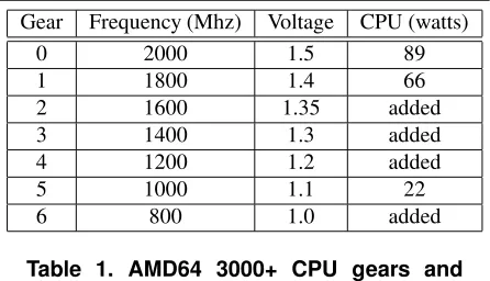
To evalute the implementation a cluster of ten servers was built using frequency scaling processors. Each node consists of the following hardware: 40 GB Maxtor EIDE 7200 RPM disk drives, ASUS K8V motherboards (on-board 1Gb NIC), 1 GB of PC3200 DDR SDRAM, and an AMD64 3000+ CPU. All nodes were interconnected on a dedicated 100 Mb switch. The entire cluster used the Linux 2.6 kernel. For frequency and voltage scaling,
the AMD PowerNowcpufreqmodule was used.
Modifi-cations were done to this module to augment the ACPI device tables from the BIOS. These modifications to add performance states, along with the original settings, are shown in Table 1. The CPU power usage in this table is from [1].
For system power measurements, two digital multi-meters (DMMs) were connected to serial ports on a non-cluster server. Custom software was created to commu-nicate with these DMMs located on this host across the network. Each meter was inserted serially in the main power line of a node to measure amperes. Thus, a max-imum of two nodes could be measured concurrently. To calculate power, a fixed supply voltage was used after first measuring voltage with one meter and obtaining little deviation (3% maximum). A TCP-based request server was created to allow the measured node to query power usage as needed. The overhead of network ac-cess is relatively small and a mechanism such as this was needed due to a lack of on-board hardware sensors on each node. Isolating the measurement activity from the measured node helps reduce the inaccuracy associ-ated with evaluating the efficiency of developed software components.
To quantify the efficiency and performance of our so-lution, a series of low-level benchmarks was performed. The first reflects the end to end cost of switching to
dif-Execution Interval (t)
5 10 15 20 30
Minimum 0.3 0.3 0.4 0.4 1.1
Average 1.9 3.5 4.8 6.5 9.2
Maximum 12.7 17.3 16.1 17.9 18.1
Table 2. Minimum, average and maximum time (milliseconds) to determine the LP solution on one node with different execu-tion intervals (seconds).
ferent gears. This cost was measured by first
construct-ing a kernel module that utilized the cpufreq
notifica-tion mechanism to measure the internal kernel cost for state changes. Our implementation cost was measured
usingagentctl to control gear changes. The measured
values from the LPA ranged from 23-363 microseconds. A gear change to either one immediately above or one below from the current was typically the most efficient change when considering the end-to-end cost. This con-firms the incremental model used to maintain the target power in the LPA. Even so, the maximum overhead im-posed by the LPA is negligible and in the worst case, represents only 6.5% of the total time cost to switch
gears usingcpufreq. This module handles the low-level
architectural details to control the frequency and volt-age changes in the processor. Note that there is addi-tional overhead to connect and disconnect from shared
memory by agentctl that added between 164-242
mi-croseconds. The GPA only incurs this cost once when first started.
0 2 4 6 8 10 12
0 5 10 15 20 25 30 35
Execution Time (milliseconds)
Runtime Interval (seconds) Measured LP Solution Performance
1 node 2 nodes 4 nodes 6 nodes 8 nodes 10 nodes
Figure 3. Execution run times to solve the allocation problem with increasingn.
time decreases due to cache behavior. Running the algo-rithm more often allows adjustments to node power lim-its to meet demand more quickly. This, in turn, balances the power more efficiently and is the reason the five sec-ond interval is the default.
Intuitively, the general problem size grows as the number of nodes increases due to the additional con-straints. In Figure 3, the same measurement method as the prior result was used but in addition, multiple clus-ter nodes were each configured with a GPA to broadcast data. There is a slight variation that grows as the run-time interval increases, but run-times are typically clustered near the same execution time. There is no reason to as-sume a cluster of 64 nodes is solvable in the 2 millisec-ond range, but the data does support lowering the inter-val to make the allocation mechanism as responsive as possible.
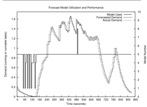
To consider the precision of the short-term forecast method, a series of ten models was constructed and workload data was fed into each of these models simul-taneously. There were two model variants, one relied on a weighted average and the other used a moving average based on a last specified number of values. The differ-ent models were generated with either differdiffer-ent weights or moving average window sizes. These models were then utilized for each inbound update from all nodes and a quick sort performed to find the model with the least mean square error when determining the new node local power limit. Figure 4 shows Model 5, a weighted
aver-age withα= 0.9, was the most effective to both classify
0 0.2 0.4 0.6 0.8 1 1.2 1.4 1.6
0 60 120 180 240 300 360 420 480 540 600 660 720 780 840 900 960 0 1 2 3 4 5 6 7 8 9 10
Demand (running or runnable tasks)
Model Number
Time (seconds) Forecast Model Utilization and Performance
Model Used Forecasted Demand Actual Demand
Figure 4. Forecast model utilization.
prior workload and make a prediction for the next inter-val. Notice that three other models were selected dur-ing this benchmark, although the total time they were used was small relative to Model 5. The global power limit was changed during this, and all other results,
us-ing theagentctltool. In addition, the standard workload
applied in this and remaining results was a gcc compiler run of the linux kernel. It is expected that changing the global allocation interval would likely impact the esti-mation model; however, the same model selection pro-cess would still choose the most applicable model dy-namically.
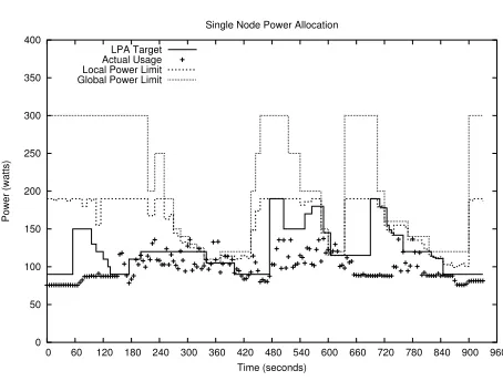
Utilizing this same data, the effectiveness of the LPA in maintaining the limit on a single node is shown in
Figure 5. For this and all other results,Lmin = 90and
Lmax = 190. These values were approximated using
cpuburn[30]. Notice as G decreases and node
work-load exists,Lsubsequently decreases between 220 and
360 seconds into the run. The measured power usage
ex-ceededLwithin three intervals due to a high power
tar-get and accumulated feedback error in the LPA. This is not a deficiency of the global allocation mechanism or policy, but does represent the most severe conditions that could occur when considering an LPA policy. It is also
important to consider that L represents the next
inter-val limit while usage is a measure of the last interinter-val. To maintain the indicated power usage, the CPU gear lization is shown in Table 3. The full spectrum was uti-lized with lower gears used when idle. There was a min-imum of 5 seconds imposed between gear changes ex-cept when the current node usage temporarily exceeded
0 50 100 150 200 250 300 350 400
0 60 120 180 240 300 360 420 480 540 600 660 720 780 840 900 960
Power (watts)
Time (seconds) Single Node Power Allocation
LPA Target Actual Usage Local Power Limit Global Power Limit
Figure 5. Single node effectiveness adher-ring to the local power limit.
Gear Count Time (msec) %
0 29 578,863 58.88
1 42 92,344 9.39
2 19 51,213 5.21
3 11 70,152 7.14
4 9 19,046 1.94
5 8 39,152 3.99
6 4 132,275 13.46
Table 3. LPA state utilization performance.
second.
In Figure 5, notice that as recovery in G occurred
near t = 430, the node power limit subsequently
in-creased for the next interval. Neart= 500andt= 600,
the global power supply again forced node power
reduc-tions for bothT andL. Because demand was high, we
still try to boost throughput even with little difference between the global and local power limits. In this and
all other results, global power reserve isR = 5. A site
with a more conservative requirement could make this higher.
To quantify the results with multiple servers, two
cluster nodes were used withG = 400watts. The
re-sults, shown in Figure 6, reflect that even under high load the resultant aggregate local power limits of both nodes follows any degredation in the global power limit.
When Node 1 first enters the cluster, at t = 20, it
0 100 200 300 400 500
0 60 120 180 240 300 360 420 480 540 600 660 0 1 2 3 4 5 6 7 8 9 10
Power (watts)
Demand (running or runnable tasks)
Time (seconds) Multiple Node Power Allocation
Global Power Limit Local Power Limit 1 Local Power Limit 2 Node Demand 1 Node Demand 2 Total Power Allocated
Figure 6. Multiple node power allocation with varying workloads and global power fluctuations.
ceives nearly the maximum allocation. Its limit subse-quently decreases given its workload and no aggregate
work to be performed. Notice that from nearlyt = 100
tot= 180, the power limit for Node 2 is atLmaxwhile
Node 1 is idle with a limit ofLmin. As demand on both
nodes rises to approximately the same level, the node lo-cal power limits are balanced appropriately. This situa-tion is later reversed when the demand on Node 2 falls while Node 1 continues processing. Later, as both nodes
become idle and the global power supply increases,L
on both nodes subsequently increases to slightly below
Lmax, with the aggregate limit well belowG. This
al-lows either node to quickly make use of available power as needed and rapidly react to additional processing re-quirements.
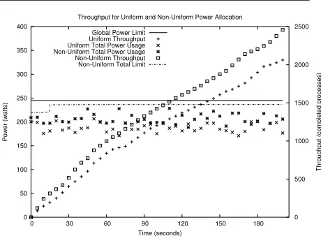
With non-uniform power allocation, it is possible to leverage the available power to increase throughput. To illustrate this benefit, two cluster nodes were configured withL = 120watts each. The value forG was fixed
at 245 watts (includes a 5 watt global reserve) so each node had an equal power allocation. Next, the standard load was applied to one of the nodes and the LPA was used to manage to the assigned local power limit. On
both nodes, the GPA was configured to not changeLand
the results are shown in Figure 7. In addition, this same graph shows the result of running the GPA to manipulate the local node power limit according to our model. No-tice the total power allocated, when the load is applied to
0 50 100 150 200 250 300 350 400
0 30 60 90 120 150 180 0
500 1000 1500 2000 2500
Power (watts)
Throughput (completed processes)
Time (seconds)
Throughput for Uniform and Non-Uniform Power Allocation
Global Power Limit Uniform Throughput Uniform Total Power Usage Non-Uniform Total Power Usage Non-Uniform Throughput Non-Uniform Total Limit
Figure 7. Throughput benefit using non-uniform power allocation.
power allocation scheme uses more than or equal to the power of the uniform method. However, from the start of the run, the node with load can easily transition to higher gears and increase throughput due to the higher local limit. The local power limit for the other idle node was
forced toLmin. After just 200 seconds, the workload
was terminated and the resultant throughput, in number of completed processes, shows a 16% gain using the dy-namic, non-uniform power allocation method.
The throughput gain in the previous result is depen-dent on the particular application and the length of time needed to service normal demand. Long running pro-cesses, such as web or database servers, would experi-ence a boost in throughput based on the relative work-loads on each server (or multiple servers in the whole cluster). A data center with a hetereogenuos mix of ap-plications, with non-migratable workloads, would ex-perience gains if one server is busier than others dur-ing different time periods. This is the typical configura-tion at many hosting centers that provide managed, ded-icated services for customers. Such configurations are typically used to address security, performance, reliabil-ity, or other customer requirements.
6. Summary
This paper investigates a non-uniform, automatic dis-tribution of power for server clusters based on forecasted workload. Because the speed and performance of servers continues to increase, the additional power such servers
consume must be accounted for in both the provisioning and financial planning processes. Power can be an auto-matically controlled resource within defined limits. Ef-fective control yields greater utilization within the global limit as well as boosts application throughput. It is not always necessary to run a server at maximum perfor-mance. As a result, safe overprovisioning can occur by managing a cluster of servers to meet power limits.
A number of improvements are planned for the cur-rent implementation. First, a more robust local power mechanism based on multiple power scalable compo-nents is being developed. This controller will account for the power usage and performance of multiple devices. The second enhancement is to ensure a tight bound on the local limit. This is possible by forcing CPU idle time at a per-task level with the objective to increase lo-cal throughput. These throughput gains are possible by slowing down higher power consuming tasks. The final planned improvements are to synchronize simultaneous local limit changes and supplement the short-term fore-cast model with additional medium or long-term mod-els.
We have presented a global power allocation mecha-nism based on both local and global power limits. The additional throughput gains possible from a strategy to manage power limits can increase the computational effectiveness of data centers that have non-migratable workloads, suffer from the inability to expand their power infrastructure, or seek an effective solution to transition from ad-hoc management methods. Our dis-tributed and autonomic power control policy not only yields gains in throughput but also handles balancing the load across a heterogeneous mix of applications and ar-chitectures.
References
[1] AMD Athlon 64 processor data sheet. http://www. amd.com/us-en/assets/content_type/ white_papers_and_tech_docs%/24659.PDF, February 2004.
[2] F. Bellosa. The benefits of event-driven energy account-ing in power-sensitive systems. InProceedings of the 9th ACM SIGOPS European Workshop, September 2000. [3] M. Berkelaar. Mixed integer programming solver.
http://groups.yahoo.com/lp_solve/, Jan-uary 2005.
[5] D. Bradley, R. Harper, and S. Hunter. Workload-based power management for parallel computer systems. IBM Journal of Research and Development, 47(5):703–718, September 2003.
[6] E. V. Carrera, E. Pinheiro, and R. Bianchini. Conserving disk energy in network servers. InProceedings of Inter-national Conference on Supercomputing, pages 86–97, San Fransisco, CA, 2003.
[7] J. S. Chase, D. C. Anderson, P. N. Thakar, A. Vahdat, and R. P. Doyle. Managing energy and server resources in hosting centers. InSymposium on Operating Systems Principles, pages 103–116, 2001.
[8] C. Ellis. The case for higher-level power management.
Proceedings of the 7th Workshop on Hot Topics in Oper-ating Systems, March 1999.
[9] E. M. Elnozahy, M. Kistler, and R. Rajamony. Energy-efficient server clusters. InWorkshop on Mobile Com-puting Systems and Applications, February 2002. [10] M. E. Femal and V. W. Freeh. Safe overprovisioning:
Using power limits to increase aggregate throughput. InWorkshop on Power-Aware Computer Systems, Dec. 2004.
[11] K. Flautner, S. Reinhardt, and T. Mudge. Automatic performance-setting for dynamic voltage scaling. In Pro-ceedings of the 7th Conference on Mobile Computing and Networking MOBICOM ’01, July 2001.
[12] J. Flinn and M. Satyanarayanan. Energy-aware adapta-tion for mobile applicaadapta-tions. InSymposium on Operating Systems Principles, pages 48–63, 1999.
[13] J. Flinn and M. Satyanarayanan. Powerscope: A tool for profiling the energy usage of mobile applications. In Pro-ceedings of the Second IEEE Workshop on Mobile Com-puting Systems and Applications, February 1999. [14] C. Gniady, Y. C. Hu, and Y.-H. Lu. Program counter
based techniques for dynamic power management. In
Proceedings of the 10th International Symposium on High-Performance Computer Architecture, Feb. 2004. [15] F. Gruian. Hard real-time scheduling for low-energy
us-ing stochastic data and DVS processors. InProceedings of the International Symposium on Low-Power Electron-ics and Design ISPLED ’01, August 2001.
[16] S. Gurumurthi, A. Sivasubramaniam, M. Kandemir, and H. Franke. Dynamic speed control for power manage-ment in server class disks. InProceedings of Interna-tional Symposium on Computer Architecture, pages 169– 179, June 2003.
[17] S. Gurumurthi, A. Sivasubramaniam, M. Kandemir, and H. Franke. Reducing disk power consumption in servers with DRPM.IEEE Computer, pages 41–48, Dec. 2003. [18] http://www.acpi.info. Advanced Configuration and
Power Interface Specification, Revision 3.0. Hewlett-Packard Corporation, Intel Corporation, Microsoft poration, Phoenix Technologies Ltd., and Toshiba Cor-poration, September 2004.
[19] C. Im, H. Kim, and S. Ha. Dynamic voltage schedul-ing technique for low-power multimedia applications us-ing buffers. InProceedings of the International Sympo-sium on Low-Power Electronics and Design ISPLED ’01, August 2001.
[20] R. Joseph and M. Martonosi. Run-time power estimation in high performance microprocessors. InProceedings of the International Symposium on Low-Power Electronics and Design ISPLED ’01, August 2001.
[21] N. Kandasamy, S. Abdelwahed, and J. P. Hayes. Self-optimization in computer systems via on-line control: Application to power management. InProceedings of the 1st IEEE International Conference on Autonomic Com-puting (ICAC ’04), pages 54–61, May 2004.
[22] C. Lefurgy, K. Rajamani, F. Rawson, W. Felter, M. Kistler, and T. W. Keller. Energy management for commerical servers.IEEE Computer, pages 39–48, Dec. 2003.
[23] J. Markoff and S. Lohr. Intel’s huge bet turns iffy. New York Times Technology Section, September 29, 2002. Section 3, Page 1, Coumn 2.
[24] R. J. Minerick, V. W. Freeh, and P. M. Kogge. Dynamic power management using feedback. In Workshop on Compilers and Operating Systems for Low Power, pages 6–1–6–10, Charlottesville, Va, September 2002. [25] A. Miyoshi, C. Lefurgy, E. V. Hensbergen, R. Rajamony,
and R. Rajkumar. Critical power slope: Understanding the runtime effects of frequency scaling. InProceedings of the 16th International Conference on Supercomputing, pages 35–44, 2002.
[26] T. Pering, T. Burd, and R. Brodersen. The simulation and evaluation of dynamic voltage scaling algorithms. In
ISLPED 1998, Aug. 1998.
[27] E. Pinheiro, R. Bianchini, E. Carrera, and T. Heath. Load balancing and unbalancing for power and performance in cluster-based systems. InProceedings of the Workshop on Compilers and Operating Systems, September 2001. [28] E. Pinheiro, R. Bianchini, E. V. Carrera, and T. Heath.
Dynamic cluster reconfiguration for power and perfor-mance. InCompilers and Operating Systems for Low Power, September 2001.
[29] J. Pouwelse, K. LangenDoen, and H. Sips. Energy pri-ority scheduling for variable voltage processors. In Pro-ceedings of the International Symposium on Low-Power Electronics and Design ISPLED ’01, August 2001. [30] R. Redelmeier. cpuburn.
http://pages.sbcglobal.net/redelm/, June 2001.
[31] V. Sharma, A. Thomas, T. Abdelzaher, and K. Skadron. Power-aware QoS management in web servers. In24th Annual IEEE Real-Time Systems Symposium, Cancun, Mexico, Dec. 2003.