ABSTRACT
BABAEI, SAMAN. Control Structures for VSC-based FACTS Devices under Normal and Faulted AC-systems. (Under the direction of Dr. Subhashish Bhattacharya.)
Control Structures for VSC-based FACTS Devices under Normal and Faulted AC-systems
by Saman Babaei
A dissertation submitted to the Graduate Faculty of North Carolina State University
in partial fulfillment of the requirements for the degree of
Doctor of Philosophy
Electrical Engineering
Raleigh, North Carolina 2014
APPROVED BY:
_______________________________ ______________________________ Dr. Subhashish Bhattacharya Dr. Iqbal Husain
Committee Chair
DEDICATION
BIOGRAPHY
The author, Saman Babaei, was born in Tehran, Iran. He received the B.Sc. and M.Sc. degrees in electrical engineering from Iran University of Science and Technology, Tehran Iran, and Chalmers University of Technology, Gothenburg, Sweden respectively. He had four years of working experience in the area of power system operation and protection.
ACKNOWLEDGMENTS
This work has been done at the Department of Electrical and Computer Engineering at North Carolina State University.
I would like to express my sincere gratitude to my advisor Professor Subhashish Bhattacharya for his guidance and support throughout the course of this work. He particularly taught me how to strategize solving a scientific problem and also how to conduct a research independently. It has been a great pleasure to work at the National Science Foundation funded Future Renewable Electric Energy Delivery and Management (FREEDM) Systems Center. I would like to acknowledge the effort of all the FREEDM faculty members to create and maintain an excellent research and education environment. I would like to gratefully thank Professor Iqbal Husain for the innumerable technical discussions that I had with him and also for his valuable help and support when I was looking for a job. I would like to thank Dr. Colin Schauder for giving me some time out of his precious time to discuss about my research whenever I met him at a conference or a meeting.
My sincere gratitude goes toward all the people at the FREEDM System centers for providing really nice and friendly atmosphere specially my friends Dr. Babak Parkhideh, Nima Yousefpoor, Hesam Mirzaee, Behzad Nabavi, Maziar Vanooni, Vahraz Zamani, Ghazal Fallahi, Mohammad Etemadrezaei, Daniel Fregosi, and Nicolas Park. I particularly would like to thank Karen Autry for her help and for her friendly good morning on every single day that I came to the FREEDM Systems Center.
TABLE OF CONTENTS
LIST OF TABLES ... ix
LIST OF FIGURES ... x
Chapter 1: Introduction ... 1
1.1 Background ... 1
1.2 Relevance ... 2
1.3 Contributions... 4
1.4 Organization ... 5
Chapter 2: Review of different control structure for the STATCOM ... 7
2. 1 Introduction ... 7
2. 2 Derivation of the STATCOM Mathematical Model ... 8
2.2.1 Stationary (αβ) and synchronous (dq) coordinate systems ... 8
2.2.2 STATCOM equations and controllers ... 13
2. 3 Comparison between the PWM-controlled and angle-controlled STATCOM performances ... 21
2.3.1 PWM-controlled VSC-based STATCOM ... 22
2.3.2 Line-frequency-switched pulse inverter ... 24
2.3.2.1 PSCAD simulation results of the angle-controlled STATCOM ... 28
2.3.2.2 Real Time Digital Simulation (RTDS) results of the angle-controlled STATCOM ... 30
2.3.2.3 Transient Network Analyzer (TNA) Results of the Angle-Controlled STATCOM ... 35
2. 4 Appendix (2-A) ... 42
Chapter 3: Dual Angle Control for Line-Frequency-Switched Static Synchronous Compensators under System Faults ... 48
3. 1 Introduction ... 48
3. 2 Angle-controlled STATCOM under normal and system faults ... 51
3.2.1 Description of Conventional Angle-Controller Structure ... 51
3.2.2 Angle-Controlled STATCOM under Unbalanced Conditions and System Faults………... ... 53
3. 4 Proposed Control Structure ... 60
3.4.1 Derivation of STATCOM equations in the negative synchronous frame ... 60
3.4.2 Control input to control the negative sequence current ... 63
3.4.3 Control structure ... 66
3. 5 PSCAD/EMTDC simulation results ... 67
3. 6 Experimental verification ... 71
3.6.1 Brief description of Transient Network Analyzer (TNA)... 71
3.6.2 Experimental Results ... 74
3. 7 Summary ... 81
3. 8 Appendix (3-A) ... 83
Chapter 4: DC-side Series Active Power Filter for STATCOM Performance under System Faults ... 84
4.1 Introduction ... 84
4.2 VSC under unbalanced conditions ... 88
4.3 Proposed Control Structure Development ... 93
4.3.1 Derivation of STATCOM equations in the negative synchronous frame ... 93
4.3.2 Proposed Controller ... 96
4.3.3 Controller Design Consideration ... 98
4.4 PSCAD simulation results ... 103
4.5 Summary ... 116
Chapter 5: Oscillatory Angle Control Scheme for PWM Static ... 117
Synchronous Compensators under Unbalanced Conditions and System Faults ... 117
5.1 Introduction ... 117
5.2 Backgrounds on controlling the VSC under unbalanced conditions ... 121
5.3 Analysis of VSC under unbalanced operating conditions ... 122
5.4 Voltage spectral content ... 126
5.5 Proposed Control Structure Development ... 129
5.5.1 Derivation of STATCOM equations in the negative synchronous frame ... 129
5.5.2 DC-link voltage dynamics ... 132
5.5.3 Proposed Controller ... 136
5.6 PSCAD Simulation Results ... 140
5.7 Hardware-In-the-Loop- test ... 145
5.8 Summary ... 147
5.9 Appendix 5-A... 150
Chapter 6: Instantaneous Fault Current Limiter for PWM-Controlled VSCs Faults... 151
6.1 Introduction ... 151
6.2 Proposed Control Structure ... 153
6.3 PSCAD simulation results ... 157
6.4 Hardware-In-the-Loop- test ... 163
6.5 Summary ... 168
Chapter 7: A control structure to increase the controllability range of the Unified Power Flow Controller ... 169
7.1 Introduction ... 169
7.2 Basic principle of the UPFC ... 170
7.3 UPFC steady state operation ... 171
7.4 Series inverter dynamics ... 173
7.5 Different series inverter control structures ... 175
7.5.1 Cross-coupling control method ... 175
7.5.2 Advanced control method ... 176
7.6 Shunt inverter (STATCOM) controller ... 181
7.7 Simulation system configuration ... 184
7.8 Simulation results of the UPFC connected to the 2-Machine AC-System ... 186
7.9 UPFC operational limit ... 194
7.10 Proposed Solution ... 195
7.11 Simulation Results of the UPFC Connected to the New York Power Authority 3-Bus Ac-system model ... 199
7.12 Summary ... 208
Chapter 8: Summary of the work ... 209
LIST OF TABLES
Table 2-1. Converter 1 output voltage phase shifting ... 44
Table 2-2. Converter 2 output voltage phase shifting ... 44
Table 2-3. Converter 3 output voltage phase shifting ... 45
Table 2-4. Converter 4 output voltage phase shifting ... 45
Table 3-1: calculation and simulation results of one three level NPC 48-pulse inverter ... 59
Table 4-1: calculation and simulation results of one three level NPC 48-pulse inverter ... 92
Table 4-2: Simulation parameters ... 106
Table 5-1 Test system parameters ... 142
LIST OF FIGURES
Figure 2-1. Instantaneous current vector ... 9
Figure 2-2. Instantaneous vectors in αβ coordinate system ... 10
Figure 2-3. Instantaneous vectors in synchronous frame (dq) ... 13
Figure 2-4. STATCOM connected to the AC-system ... 14
Figure 2-5. Vector controlled STATCOM control structure ... 16
Figure 2-6. Angle controller ... 20
Figure 2-7. 2-level VSC-based PWM controlled inverter ... 22
Figure 2-8. 2-level VSC-based PWM controlled inverter voltage spectrum with different modulation index ... 23
Figure 2-9. Power circuit of the NYPA three-level NPC 48-pulse inverter ... 25
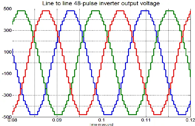
Figure 2-10. 48-pulse inverter line to line output voltages ... 27
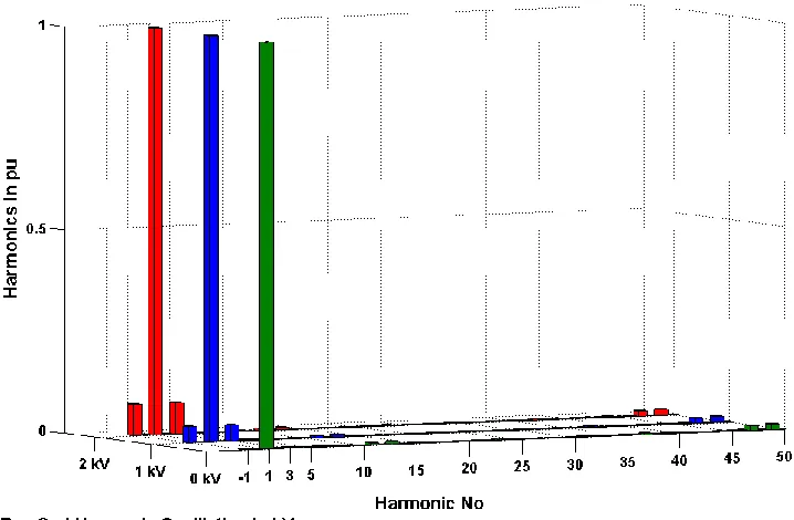
Figure 2-11. 48-pulse inverter output voltage harmonic content ... 27
Figure 2-12. The angle-controlled STATCOM connected to the NYPA 3-bus AC system. Per unit values are based on 345kV, and 100 MVA ... 28
Figure 2-13. 48-pulse angle-controlled STATCOM performance with different current references. Per unit values are based on 345kV, and 100 MVA ... 29
Figure 2-14. RTDS Racks at NCSU ... 31
Figure 2-15. Rack 1 (column (a)), and 2 (column (b)) processor usage for the angle-controlled STATCOM simulation ... 31
Figure 2-16. Angle-controlled STATCOM performance with iq=0 ... 32
Figure 2-17. Angle-controlled STATCOM performance with iq=1 pu inductive ... 32
Figure 2-18. Angle-controlled STATCOM performance with iq=-1 pu capacitive ... 33
Figure 2-19. Angle-controller performance in transition from capacitive (iq=-1 pu) to zero current ... 33
Figure 2-20. Angle-controlled STATCOM performance in transition from zero current to fully inductive (iq=1pu) ... 34
Figure 2-21. Interface of Control equipment to TNA ... 36
Figure 2-22. Scaled down model of the NYPA 3-bus AC system used for experimental verification ... 36
Figure 2-23. Inverter and control panels ... 37
Figure 2-24. One-Line Diagram Screen... 38
Figure 2-26. Operator Control Screen for STATCOM ... 38
Figure 2-27. Operator Control Screen for UPFC ... 38
Figure 2-28. STATCOM transition from inductive mode Iq=0.6 pu to capacitive mode Iq=-0.7 pu... 39
Figure 2-29. The STATCOM transition from inductive mode Iq=0.6 pu to zeroe current Iq=0 ... 40
Figure 2-30. The STATCOM transition from zero current Iq=0 pu to capacitive mode Iq=-0.7... 40
Figure 2-31. NPC converter output voltage ... 42
Figure 2-32. illustrative harmonic elimination of the 48-pulse inverter using the gate drive phase shift and also auxiliary and shunt transformers phase shifting. All the harmonics up to the 49th are illustrated. Blue, red, green, and black represent the NPC converter 1, 2, 3, and 4 respectively. ... 47
Figure 3-1. Control structure of a vector controlled (PWM) STATCOM ... 52
Figure 3-2. Control structure of an angle-controlled STATCOM ... 52
Figure 3-3. 48-pulse inverter line to line output voltages ... 52
Figure 3-4. Angle-controlled STATCOM performance with two different instantaneous reactive current (Iq) references ... 54
Figure 3-5. Equivalent circuit of a VSC connected to AC system ... 56
Figure 3-6. Equivalent circuit of the 3-Level NPC VSC used for calculation of the fundamental negative sequence voltage vector at VSC output terminals ... 59
Figure 3-7. 48-pulse inverter output voltage harmonic content with different 2nd harmonic oscillations added to the DC-link voltage ... 60
Figure 3-8. STATCOM equivalent circuit with series negative sequence voltage sources .... 61
Figure 3-9. STATCOM instantaneous vectors in the negative synchronous frame ... 61
Figure 3-10. Bode plots of the DC-link voltage perturbation against α perturbation around a capacitive (a)/inductive (b) equilibrium point ... 65
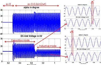
Figure 3-11. DC-link voltage 2nd harmonic oscillations generated by introducing 2nd harmonic oscillations to the α in both capacitive and inductive operation modes ... 65
Figure 3-12. Proposed Control structure ... 68
Figure 3-13. 3-bus AC system model. All the pu values are based on 345 kV and 100 MVA ... 69
Figure 3-15. STATCOM performance with (b) and without (a) proposed DAC when STATCOM is working in inductive mode and SLG fault at phase C is applied right at
STATCOM bus. (PSCAD/EMTDC simulation results) ... 72 Figure 3-16. STATCOM performance with (b) and without (a) proposed DAC when
STATCOM is working in capacitive mode and SLG fault at phase C is applied in the middle of the Marcy-Bus1 345 kV outgoing transmission line in the 3-bus AC system .
(PSCAD/EMTDC simulation results)... 72 Figure 3-17. STATCOM performance with (b) and without (a) proposed DAC when
STATCOM is working in capacitive mode and SLG fault at phase C is applied in the middle of the Marcy-Bus2 345 kV outgoing transmission line in the 3-bus AC system .
(PSCAD/EMTDC simulation results)... 73 Figure 3-18. Interface of Control equipment to TNA ... 74 Figure 3-19. Control and magnetic panels ... 75 Figure 3-20. Scaled down model of the NYPA 3-bus AC system used for experimental verification ... 75 Figure 3-21. Power circuit topology of the inverters connected to auxiliary and shunt
transformers to construct 48-pulse output voltage waveform ... 75 Figure 3-22. STATCOM performance with and without DAC in capacitive operation mode when there is 25% of negative sequence voltage injection at STATCOM bus. All pu values are based on 12 VA and 100 V RMS (L-L) ac system. (Experimental results) ... 77 Figure 3-23. Capacitive mode performance of STATCOM under single line to ground fault with (b) and without (a) DAC. All pu values are based on 12 VA and 100 V RMS (L-L) ac system. (Experimental results) ... 78 Figure 3-24. Inductive mode performance of STATCOM under single line to ground fault with (b) and without (a) DAC. All pu values are based on 12 VA and 100 V RMS (L-L) ac system. (Experimental results) ... 79 Figure 4-1. Control structure of an angle-controlled STATCOM ... 86 Figure 4-2. Simultaneous and independent control of positive and negative-sequence voltages ... 87 Figure 4-3. Equivalent circuit of a VSC connected to AC system. ... 91 Figure 4-4. Equivalent circuit of the inverter used for calculation of the fundamental
Figure 4-9. d and q current control loop ... 102
Figure 4-10. Notch filter bode plots ... 102
Figure 4-11. Block diagram of the Phase Locked Loop ... 103
Figure 4-12. Power circuit of the NYPA three-level NPC 48-pulse inverter ... 104
Figure 4-13. The 48-pulse output voltage when the DC-link is not connected to the single phase inverter. ... 105
Figure 4-14. NYPA 3-bus AC system ... 105
Figure 4-15. STATCOM performance with and without proposed solution under phase a SLG fault right at STATCOM bus (fault location1) when STATCOM is working in capacitive (a) and inductive (b) mode of operation. The current THD reaches from 1.2% before fault to around 2.9% after fault with proposed controller in both inductive and capacitive modes ... 107
Figure 4-16. STATCOM performance with and without proposed solution under phase a SLG fault in the middle of the Marcy-Bus1 345 kV transmission line (fault location2) when STATCOM is working in capacitive (a) and inductive (b) mode of operation. The current THD reaches from 1.2% before fault to around 2.3% after fault with proposed controller in both inductive and capacitive modes ... 108
Figure 4-17. STATCOM performance with and without proposed solution under Line to Line fault between phase b , and c in the middle of the Marcy-Bus1 345 kV transmission line (fault location2) when STATCOM is working in capacitive (a) and inductive (b) mode of operation. The current THD reaches from 1.2% before fault to around 23% after fault with proposed controller in both inductive and capacitive modes. ... 111
Figure 4-18. STATCOM performance with (b) and without (a) proposed solution under phase a SLG fault right at STATCOM bus (fault location1) when STATCOM is working in capacitive mode of operation ... 112
Figure 4-19. STATCOM negative-sequence current and single phase inverter current and voltage under a Line to Line fault in the middle of the Marcy-Bus1 345 kV transmission line ... 114
Figure 5-1. Voltage regulation of a load sensitive to voltage dip using a PWM VSC-based STATCOM ... 119
Figure 5-2. Simultaneous controlling of Neg. Seq. and Pos. Seq. voltages... 120
Figure 5-3. Equivalent circuit of an VSC connected to AC system ... 125
Figure 5-4. 2- level inverter with variable AC-sources used to calculate the generated negative sequence voltage at VSC terminals ... 126
Figure 5-6. Inverter output voltage with modulation index of 0.8(a), and 0.9 (b) and switching frequency of 1260 Hz when different percentages of 2nd harmonic oscillations
(with respect to the DC-link average voltage ) are added to the DC-link voltage. ... 128
Figure 5-7. STATCOM equivalent circuit with series negative sequence voltage sources .. 130
Figure 5-8. STATCOM instantaneous voltage vectors in the negative synchronous reference frame ... 130
Figure 5-9. STATCOM vectors in the positive synchronous frame ... 130
Figure 5-10. Bode plots of the DC-link voltage perturbation against α perturbation around different inductive and capacitive equilibrium points. Positive and negative Iq corresponds to the capacitive and inductive mode of operations respectively ... 134
Figure 5-11. Bode plots of the DC-link voltage perturbation against α perturbation around one capacitive (a)/inductive (b) equilibrium point with different modulation index. ... 134
Figure 5-12. DC-link voltage 2nd harmonic oscillations generated by introducing 2nd harmonic oscillations to α in both capacitive (a) and inductive (b) operation modes. ... 135
Figure 5-13. Proposed control structure... 137
Figure 5-14. Block diagram of the compensated and ... 140
Figure 5-15. Closed loop rout locus of the compensated and with three different values of i.e. 0, 90, and -90 ... 141
Figure 5-16. Single line diagram of the simulated test system ... 142
Figure 5-17. STATCOM performance with (b) and without (a) proposed controller when STATCOM is working in capacitive mode ... 143
Figure 5-18. STATCOM performance with (b) and without (a) proposed controller when STATCOM is working in inductive mode... 144
Figure 5-19. Hardware-in-the-Loop test system ... 145
Figure 5-20. Capacitive mode performance of the STATCOM under SLG fault without proposed controller. Voltage scale: 100V/div. and Current scale:5A/div. ... 146
Figure 5-21. Capacitive mode performance of STATCOM under SLG fault with proposed controller. Voltage scale: 100V/div. and Current scale:5A/div ... 146
Figure 5-22. Inductive mode performance of STATCOM under SLG fault without proposed controller. Voltage scale: 100V/div. and Current scale:5A/div. ... 146
Figure 5-23. Inductive mode performance of the STATCOM under SLG fault with proposed controller. Voltage scale: 100V/div. and Current scale:5A/div. ... 147
Figure 6-1. VSC connected to the grid ... 153
Figure 6-2. Converter equivalent circuit with series negative sequence voltage sources ... 154
Figure 6-3. Proposed control structure... 156
Figure 6-5. Converter performance with and without proposed controller when there is negative (a)/3rd harmonic (b) voltage injection as big as 20% of the nominal system voltage
in series with grid AC sources ... 160
Figure 6-6. Converter performance with (b) and without (a) proposed controller under SLG fault at phase A right at PCC ... 161
Figure 6-7. Converter performance with and without proposed controller under SLG fault at phase A right at PCC... 162
Figure 6-8. Hardware-in-the-Loop test system ... 164
Figure 6-9. Rectifier voltages and current under normal condition. Voltage scale: 100V/div. and Current scale: 10A/div. ... 164
FIGURE 6-10. PCC and DC-link voltages under SLG fault at phase A when converter works with conventional controller. Chanel 1, 2, 3, and 4 indicate the Va, Vb, Vc, and DC-link voltage respectively. Voltage scale: 100V/div... 165
FIGURE 6-11. Converter currents under SLG fault at phase A when it works with conventional controller. Chanel 1, 2, and 3indicate Ia, Ib, and Ic respectively. Current scale:10A/div. ... 165
Figure 6-12. PCC and DC-link voltages under SLG fault at phase A when converter works with the proposed controller. Chanel 1, 2, 3, and 4 indicate the Va, Vb, Vc, and DC-link voltage respectively. Voltage scale: 100V/div... 166
Figure 6-13. Converter currents under SLG fault at phase A when converter works with the proposed controller. Chanel 1, 2, and 3 indicate the Ia, Ib, and Ic respectively. Current scale:10A/div ... 166
Figure 6-14. Converter performance with conventional controller under SLG fault at phase A. Voltage scale: 100V/div. and Current scale:10A/div ... 167
Figure 6-15. Converter performance with the proposed conroller under SLG fault at phase A. Voltage scale: 100V/div. and Current scale:10A/div. ... 167
Figure 7-1. UPFC single line ... 171
Figure 7-2. Simplified model of the UPFC connected to the sending end of the transmission line... 172
Figure 7-3. Bode plots of the direct and cross transfer functions. R=4Ω, L=0.123 H ( X/R=11.6 ). The R, and L values are based on the 345 kV simulation AC-system explained in the section 7.7 ... 175
Figure 7-4. Cross-coupling controller ... 176
Figure 7-5. UPFC advanced controller ... 177
Figure 7-6. Angle-controlled STATCOM control structure ... 182
Figure 7-8. Power circuit of the UPFC used in the simulation verification. This UPFC model is developed based on the NYPA UPFC at Marcy substation ... 184 Figure 7-9. Series 48-pulse inverter control ... 186 Figure 7-10. PSCAD UPFC model developed based on the NYPA UPFC at Marcy substation connected to the 2-Machine AC-system ... 187 Figure 7-11. The UPFC performance with a step change in the d component of the series inverter voltage reference value. (The UPFC works in the voltage injection mode) ... 188 Figure 7-12. The UPFC performance with a step change in the q component of the series inverter voltage reference value. (The UPFC works in the voltage injection mode) ... 188 Figure 7-13. UPFC performance with a step change in the (active power reference). UPFC works in power flow controller mode with series inverter in cross-coupling method190 Figure 7-14. UPFC performance with a step change in the (active power reference). UPFC works in power flow controller mode and series inverter is controlled with advanced control method ... 190 Figure 7-15. UPFC performance with a step change in the (active power reference). UPFC series inverter is controlled with cross-coupling method ... 191 Figure 7-16. UPFC performance with a step change in the (active power reference). UPFC series inverter is controlled with advanced control method. ... 192 Figure 7-17. UPFC performance with a step change in the (reactive power reference). UPFC series inverter is controlled with advanced control method ... 193 Figure 7-18. UPFC performance with a step change in the (reactive power reference) when the series inverter is controlled with advanced control method. ... 193 Figure 7-19. Fundamental voltage amplitude and the output voltage THD of the simulation system 48-pulse inverter when σ increases from zero to 90˚. Per unit values are based on 345kV, and 100 MVA... 197 Figure 7-20. Proposed control structure... 198 Figure 7-21. Simulation system, UPFC model based on the NYPA UPFC at Marcy substation is connected to the NYPA 3-bus AC-system. All the per unit values are based on 100 MVA and 345kV system. ... 199 Figure 7-22. Simulated UPFC performance with different active and reactive power
references ... 200 Figure 7-23. UPFC performance when the shunt inverter operating point changes form fully capacitive to fully inductive with and without proposed solution. The desired DC-link
voltage is set to 12kv ( =27.6˚). ... 203 Figure 7-24. UPFC performance when the shunt inverter operating point changes form fully capacitive to fully inductive with and without proposed solution. The desired DC-link
Figure 7-25. UPFC performance when the shunt inverter operating point changes form fully capacitive to fully inductive with and without proposed solution. The desired DC-link
voltage is set to 11.5kv ( =22.4˚). ... 205 Figure 7-26. UPFC performance when the shunt inverter operating point changes form fully capacitive to fully inductive with and without proposed solution. The desired DC-link
Chapter 1: Introduction
1.1 Background
At the present time, by daily increasing the electricity demand, power systems are forced to operate at their full capacity which puts too much stress on the system. Moreover, generation patterns frequently result in overloading of the transmission systems that tend to incur greater losses as well as decrease in the system stability margin and security level [1]. Therefore, the power system needs to be reinforced to increase its capacity and become smarter, aware, more fault-tolerant, self-healing and statically and dynamically controllable.
The traditional alternative to reinforce the power system is to build up new power infrastructures such as transmission lines, electrical substations, and associated equipment. However, due to the environmental issues and also high cost of the reinforcing power system through the addition of the new infrastructures, the power system expansions are often restricted [1],[2].
(UPFC), can be connected in series or shunt (or a combination of the two) to achieve numerous control functions including voltage regulation, power flow control, and system damping [2]-[24]. In this way, the system performance can be considerably improved. Following are few examples of the long list of the benefits that FACTS devices offer:
- Utilizing the power system infrastructures up to their thermal limits without sacrificing the system stability and security.
- Continuous control over the system voltage profile.
-Reactive power support functionality to improve the system voltage profile, decreasing the system losses and also improving the system voltage stability
-Power flow controllability
-Power system oscillation damping
1.2 Relevance
This thesis is concerned with improving the FACTS devices performance by proposing new control structures and also converter topologies. As mentioned in the preceding section, the combination of the increasing electricity demand and restrictions in expanding the power system has urged the utility owners to use the FACTS devices.
tripped under utility system faults or severe unbalanced conditions when its reactive power support functionality is really needed.
Basically, the inverter power components and switches must be designed for the peak continuous operating current and for the peak continuous operating voltage. Generally there is a designed margin beyond this point to accommodate some percentage overload as well as specified abnormal operating condition particularly unbalanced condition and grid faults. The MVA rating of the equipment and hence the cost is derived from the product of peak voltage and current (considering the fault and unbalanced condition), regardless of whether they occur at the same time or not [26]. Hence, the appropriate controller which is capable of limiting the fault current and consequently decrease the converter design margin will significantly reduce the converter equipment rating and cost.
The other example of the challenges regarding the VSC-based FACTS devices is the controllability range of the specific type of the UPFC in which the DC-link voltage is not fixed and is regulated over the range of the values. Many of the UPFC installations around the world are of this kind. In this type of the UPFCs, the controllability range is varied with shunt inverter operating point.
1.3 Contributions
The key contributions of this thesis are enumerated as follows:
1. Design a new control structure (Dual Angle Controller) to improve the line-frequency-switched (angle-controlled) STATCOM performance under unbalanced conditions and system faults. (Chapter 3)
2. Application of the DC-side active power filters to improve the line-frequency-switched (angle-controlled) STATCOM performance under unbalanced conditions and system faults. (Chapter 4)
3. An alternative control structure to improve the PWM-controlled VSC-based STATCOMs under AC-system faults. (Chapter 5)
4. Designing an alternative controller for the PWM-controlled VSC which is capable of instantaneous limiting the negative sequence current under fault conditions. When the line voltage is distorted by the specific harmonics, this controller can also be used to eliminate those harmonics in the current spectrum.
(Chapter 6)
1.4 Organization
Followed by the introduction, chapter 2 provides a literature survey on essential topics of this research. It starts with calculating a mathematical model for generally a VSC and particularly a STATCOM connected to the grid. That is followed by introduction of the existing control structures for the STATCOM (PWM-based vector controller, and angle-controller) and discussing the pros and cons of each of them for the transmission level application. For the literature review part of this chapter which provides the basic dynamic and static equations of the STATCOM that will be used afterward in the thesis, a close look has been taken to the Dr. Colin Schauder paper [19].This paper has been referred wherever possible through this chapter.
Chapter 3 addresses the issues regarding the angle-controlled STATCOM performance under AC-system faults. It starts with calculation of the DC, and AC-sides waveforms of the STATCOM under unbalanced condition and afterward these equations are particularly used to develop the Dual angle controller (DAC). DAC limits the STATCOM fault currents and removes the DC-link voltage 2nd harmonic oscillation under severe unbalanced conditions and AC-system faults. The proposed DAC performance has been validated by the simulation and experimental results.
sequence currents under system faults. The proposed solution is validated by the simulation results.
Chapter 5 uses the basic idea of the chapter 3 to develop an alternative control structure that improves the PWM-controlled VSC-based STATCOM performance under AC-system fault conditions. The theoretical results of this chapter are supported by the simulation and Hardware-In-the- Loop-test results.
Chapter 6 proposes a control structure that improves the grid-connected PWM-controlled VSC currents Total Harmonic Distortion (THD) and removes the DC-link voltage oscillations when the input voltage is distorted by the low/high order harmonics. The input voltage harmonic can range from (-1) which corresponds to the unbalanced AC-system conditions to any high order harmonic (providing that the switching frequency is high enough). In particular, when the input voltage is unbalanced due to the fault condition, the proposed controller instantly limits the negative sequence current and removes the DC-link voltage oscillations. The proposed controller performance is validated by the precise simulation and Hardware-In-the- Loop-test results.
Chapter 2: Review of different control structure for the STATCOM
2. 1Introduction
VSC-based STATCOMs are used for voltage regulation in transmission and distribution systems. The VSC-based STATCOM operation is based on the principle that a VSC inverter can be connected between the three phase AC-system and an energy storage device such as a capacitor and controlled to exchange mainly reactive current with AC-system[19]. Basically from the power system point of view the STATCOM is seen as a controllable current source that injects (almost) 90 degrees leading or lagging current to the AC-system. This provides the capability to act as either sink or source of the reactive power to the grid. And finally this reactive power support functionality is used to regulate the AC-bus voltage at the point of connection.
2. 2Derivation of the STATCOM Mathematical Model
2.2.1 Stationary (αβ) and synchronous (dq) coordinate systems
The main function of the STATCOM is to regulate the AC-bus voltage at the point of connection by acting as a source or sink of the reactive power. From the power system point of view the STATCOM is seen as a controllable reactive current source. Reactive current is part of the current associated with reactive power and does not have any effect on the active power.
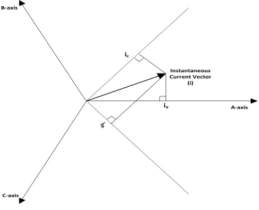
The reactive power and current are well known, however, for designing a controller with response time as fast as a fraction of a cycle a broader definition of the reactive power (current) is required which is valid on an instantaneous basis. The instantaneous active power at a point on the line is given by [19]:
(2-1)
The instantaneous reactive current can be defined as that part of the three phases current that can be eliminated at any instance without altering the real power [19]. To obtain the algebraic equation of the active and reactive instantaneous current, it is needed to transfer all the variables into a domain in which the instantaneous calculation is possible.
Figure 2-1.Instantaneous current vector
Based on instantaneous vector theory, a coordinate system is introduced in which the α-axis is coincident to the phase A-α-axis and β-α-axis is perpendicular to the α-α-axis. The transformation from abc domain to the αβ domain is defined as in:
[ ]
[
√ √
√ √ √ ]
[ ]
(2-2)
Figure 2-2 indicates the current and voltage instantaneous vectors in the αβ coordinate system. Equation (2-1) can be rewritten in the αβ-coordinate system as in:
A-axis Instantaneous
Current Vector (i)
C-axis B-axis
ia
ic
Figure 2-2.Instantaneous vectors in αβ coordinate system
( ) (2-3)
Inspection of (2-3) indicates that the instantaneous active power is the dot (scalar) product of the instantaneous voltage and current vectors in the stationary αβ-coordinate system. Therefore (2-3) can be rewritten as in:
| || | ) (2-4)
where ϕ is the angle between the instantaneous current and voltage vector. Therefore, the part of the current which is aligned with the instantaneous voltage vector (| | contributes to the active power and the remaining part (| | has no part in the active power construction and therefore is the reactive current. The instantaneous reactive power is
Instantaneous Current Vector
(i)
α-Axis (A-axis)
C-axis B-axis
iα
β-Axis
iβ
vα
vβ
Instantaneous Voltage Vector
(v)
defined as the cross product of the instantaneous voltage vector by the instantaneous current vector:
| || | (2-5)
Equation (2-5) can be rewritten as in (2-6):
(2-6)
Inspection of Figure 2-2, and considering (2-4), and (2-5) indicates that defining a rotatory co-ordinate system in which one of the axes is always coincident with instantaneous voltage vector, leads to useful separation of the variables for the active and reactive power control. Therefore, the synchronous frame (dq coordinate system) is designed in a way that d-axis is always coincident with instantaneous voltage vector and q-axis is perpendicular to the d-axis. Note should be taken that synchronous frame is not a stationary frame and d and q-axis rotate with instantaneous voltage vector. The equation (2-5), and (2-6) can be simply rewritten in the synchronous frame as in:
| | (2-7)
| | (2-8)
The instantaneous voltage and current vectors in the synchronous reference frame are illustrated in Figure 2-3.
vector and only contributes to the active power while is always perpendicular to the instantaneous voltage vector and only contributes to the reactive power.
Transformation from abc to the synchronous frame is defined as: [19],[28].
(2-9)
(2-10)
Where:
[
√ √ √ ]
(2-11)
and is the ac-bus phase locked loop output.
Writing the abc domain variables in terms of dq variables based on (2-10) and substitute them in (2-1), then the active and reactive powers in terms of dq variables are obtained as in:
(2-12)
(2-13)
Figure 2-3.Instantaneous vectors in synchronous frame (dq)
2.2.2 STATCOM equations and controllers
Figure 2-4 indicates the equivalent circuit of the STATCOM connected to the AC-system. The derivative of the STATCOM tie line currents with respect to the time can be written as in:
[ ] [ ] [ ] [ ] (2-14)
For controller design, it is always easier to work with per-unit value. The per-unit system can be obtained according the following equations [19]:
Figure 2-4.STATCOM connected to the AC-system (2-15) (2-16) (2-17) (2-18) (2-19) (2-20)
Per-unitizing (2-14) based on (2-15)-(12-20), we obtain:
[ ] [ ] [ ] [ ] (2-21)
Transferring (2-21) from abc domain to the synchronous frame based on (2-11) yields:
i
dci
an
e
ae
be
cL
R
L
R
L
R
v
av
bv
cC
dci
bi
c[ ] [ ] [ ] [ | | ] (2-22)
Rearranging (2-22) we obtain:
[ ] [ | | ] (2-23)
Inspection of equation (2-23) clearly indicates that and can easily be controlled using and respectively. The coupling between the d and q components can be removed by adding proper terms to the controller output. Feed-forwarding the | | to the d-axis controller output also improves the converter dynamic performance. Therefore, the control structure of the vector controlled (PWM-controlled) STATCOM can be illustrated as in Figure 2-5.
From the control point of view a converter can be considered as an ideal power transformer with a time delay. The output voltage of the converter is assumed to follow a voltage reference signal with an average time delay due to the PWM switching. Let's assume that the switching frequency is high enough such that the average time delay is negligible. Therefore, we will have:
[
] [
]
(2-24)
Considering the control structure of Figure 2-5 and equation (2-24), then , and
Figure 2-5.Vector controlled STATCOM control structure
( ) ( ) | | (2-25)
( ) ( ) (2-26)
These two equations show that the reference voltage of the inverter can be split into two components. One of them is obtained from the PI controller and the other one is feed-forward term to remove the coupling between d and q axis and also improve the transient response. The reference for the q component of the STATCOM current is calculated based on the required capacitive or inductive reactive power at the point of the connection. The d component reference value is calculated by a PI controller that regulates the DC-link voltage at a fixed value.
The PWM-controlled STATCOM may be uneconomical for many transmission level FACTS devices due to the high switching losses of the PWM VSCs. Apart from the PWM-controlled STATCOM; there is another STATCOM controller which is based on controlling
Vbus
d
q Iq pu
Id pu
Phase and Amplitude Calculation ∑ + -∑ +
-Id ref pu
Iqref pu
ed pu eq pu
PLL
Ө abc/dq
Inverter curent sensors PWM Switching Pattern Lpu Lpu ∑ ∑ i p s K K i p s K K
-vd pu + +
-+
Vdc pu
∑ +
-Vdc ref pu
only the angle of the output voltage. It has been shown in [19] that by a slight change of the inverter output voltage angle (α) for a controlled time; the inverter is able to provide inductive/capacitive reactive power. Basically, by controlling the α toward the positive/negative direction , for a controlled time, the DC-link voltage is driven lower/higher and therefore the VSC output voltage decreases/increases accordingly[29].In this type of inverter, the ratio between AC and DC voltages is kept constant and the VSC output voltage magnitude is varied indirectly by changing the DC-bus voltage. Since angle α is the only control input in this control strategy, it is called angle control.
Since in the angle-controlled STATCOM the inverter output voltage is controlled by changing the DC-link voltage level, it is necessary to include the DC-side equation in the STATCOM model. The instantaneous active power at the AC and DC-side of the inverter are identical. Therefore we have:
( ) (2-27)
And the DC-side circuit equation is:
(2-28)
is a shunt resistance at DC-side that models the converter losses. In all the converters the absolute value of the fundamental inverter output voltage is proportional with DC link voltage.
(2-29)
(2-30)
(2-31)
k is the factor for inverter which relates the DC-side voltage to the amplitude of the phase to neutral voltage at the inverter AC-side terminals.
Combining equations (2-22), (2-27), (2-28), (2-30), and (2-31), yields:
[ ] [ ] [ ] [ | | ] (2-32)
Rearranging (2-32), we will have:
State space equations in (2-32) are nonlinear if α is considered as one of the system input. However, by linearizing equation (2-32) around an equilibrium point, it is possible to analyze the perturbation of the d and q component of the current and also DC-link voltage about a chosen steady state point. f1, f2, and f3 are nonlinear differential equations defined in (2-33). The linearization process is carried out based on (2-34):
[ ] [ ] [ ] [ | | | | | | ] ⌈ | | ⌉ (2-34)
and therefore linearizing (2-33) based on (2-34) yields:
[ ] [ ] [ ] [ ] ⌈ | | ⌉ (2-35)
equations of (2-35), the transfer function between the perturbations ( and is calculated as in [19]:
( ) (2-36) Where [19]: (2-37) (2-38)
Note should be taken that to obtain this transfer function the AC-system cupper losses and also converter switching losses are ignored ( , , and ). Having obtained the transfer function between the and and using the well-known
control rules it is possible to design an appropriate controller. Figure 2-6 illustrates the control structure of the STATCOM working with angle controller.
∑
I
q ref2
1
K
K
S
α
∑
Phase
Locked Loop
V
busInverter
Voltage
Command
I
inverter
I
q+
-+
+
2. 3Comparison between the PWM-controlled and angle-controlled STATCOM performances
2.3.1 PWM-controlled VSC-based STATCOM
Figure 2-7 indicates a simple 2-level VSC-based inverter. This inverter is controlled using the PWM technique. The link is connected to the series connection of two DC-voltage sources. In this inverter the DC-link DC-voltage is being chopped with the PWM pulses to any arbitrary voltage vector with desired amplitude and angle.
Figure 2-7.2-level VSC-based PWM controlled inverter
Figure 2-8 indicates the voltage spectrum of this inverter with different modulation index. The switching frequency is set to 21 times of the line frequency (21×60=1260). As can be seen in this figure the harmonics value around the switching frequency and its multiple is
Ea Eb Ec
(VSI)
very large. Usually the switching frequency is set to a large number to push the harmonics far from the line frequency. The inductor that connects the inverter to the grid is seen as the open circuit for the high order harmonics and prevents them to reach to the grid (providing that the switching frequency is large enough). However, the larger the switching frequency the more converter losses we will have. Therefore, for transmission level applications the PWM-controlled inverter is uneconomical.
2.3.2 Line-frequency-switched pulse inverter
It was mentioned in the previous section that the PWM-controlled inverters are uneconomical for the transmission level application due to the high converter losses. The type of the inverter that suits for the transmission level application must have two basic following characteristics:
1- Low switching frequency (low converter losses)
2- High quality voltage at Point of Common Coupling (PCC) (low Total Harmonic Distortion(THD))
With PWM-controlled inverters we could not have both of the mentioned characteristics at the same time. To decrease the voltage THD at PCC we had to increase the switching frequency that lead to high converter loses. There is another type of the inverter that perfectly meets the mentioned transmission level requirements. The line –frequency-switched pulse inverters synthesize a very high quality voltage at their output terminals with switching frequency as low as the line frequency.24, and 48-pulse inverters are commonly used in the FACTS devices. A group of Neutral Point Clamped (NPC) inverters are electromagnetically coupled using transformers to synthetize the high quality output voltage. The inverter output voltage magnitude is changed indirectly by changing the DC-link voltage level.
Figure 2-9.Power circuit of the NYPA three-level NPC 48-pulse inverter[30].
Compensator (CSC) at the Marcy substation. This inverter has been used in different chapter of the thesis. The entire angle controlled STATCOM simulation and experimental results throughout the thesis are based on this 48-pulse inverter. The UPFC model used in the last chapter of the thesis is also based on this inverter.
Figure 2-10.48-pulse inverter line to line output voltages
Figure 2-11 indicates the harmonic content of the 48-pulse inverter output voltage. As it can be seen in this figure the quality of the output voltage is very high and there is not any considerable high or low order harmonics rather than the fundamental frequency. The output voltage THD is 3%.
2.3.2.1 PSCAD/ EMTDC simulation results of the angle-controlled STATCOM
In this part of the thesis the 48-pulse inverter has been modeled in the PSCAD/EMTDC platform and has been controlled with angle control structure to have the STATCOM functionality. This STATCOM has been connected to the reduced order 3-bus AC-system model of the NYPA power system as shown in Figure 2-12. All the per unit values are based on 100 MVA, and 345 kV base system.
Figure 2-12.The angle-controlled STATCOM connected to the NYPA 3-bus AC system. Per unit values are based on 345kV, and 100 MVA.
Marcy Bus1 0.01 pu
0.0183 pu 0.0329 pu
0.039 pu
0.1135 pu
0.067 pu 0.0077 pu
Bus 2
0.788 pu
1.173 pu 1.173 pu STATCOM
0.0609 pu 0.788 pu
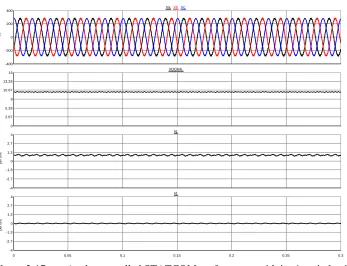
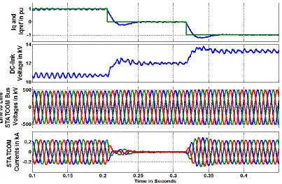
Results in Figure 2-13 illustrate the STATCOM performance under different control command. Initially STATCOM works in the inductive mode of operation and absorbs 1 pu (167.347 A equivalent to 100 MVA reactive power) of inductive current form the grid. The reference of iq is set to be zero at around t=0.21 seconds and finally at around t=0.32 seconds it starts to work in capacitive mode of operation and injects 1 pu of capacitive current to the grid. As can be seen in this figure the reactive current follows its reference value quickly and smoothly. It is also important to note that the DC-link voltage value is not fixed and changes over the range of the values. That is due to the reason that the angle controller changes the inverter output voltage indirectly by changing the DC-link voltage level.
2.3.2.2 Real Time Digital Simulation (RTDS) results of the angle-controlled STATCOM
The 48-pulse inverter along with the angle controller has been implements in the RTDS platform. Four GPC processor cards plus two PB5 cards have been used to simulate the entire angle-controlled STATCOM along with the 3-bus AC-system. 48 GTO valves are distributed between two small time step bridge boxes. Small time step bridge box is designed for the power electronics simulations and all the components inside the bridge boxes are ran with small time step (very fast). The number of the small time component that can be placed inside a bridge box cannot exceed a specific number (this number varies depending on the processor usage of each component). In our case for simulation of the 4 NPC inverters and auxiliary and shunt transformers 3 bridge boxes have been used. The 3-bus AC system has been simulated in the large time step. Bridge boxes must be connected to each other using the transmission line or transformer model. The small time step part of the simulation is also being connected to the large time step part using a transmission line. These transmission lines do not exist in the real model and although their impedance have been set to the minimum possible value, but they affect the simulation results. The other constraint in our RTDS simulation was that using too many small time step components dramatically increases the minimum possible time step. In our case it was not possible to lower the time step below the 70 μs.
Figure 2-14.RTDS Racks at NCSU
(a) (b)
Figure 2-16. Angle-controlled STATCOM performance with iq=0
Figure 2-17. Angle-controlled STATCOM performance with iq=1 pu inductive
0 0.05 0.1 0.15 0.2 0.25 0.3
-4 -2.7 -1.3 0 1.3 2.7 4 p e r u n it Id -4 -2.7 -1.3 0 1.3 2.7 4 pe r un it Iq 0 2.67 5.33 8 10.67 13.33 16 kV VDClink -400 -200 0 200 400 kV
VaVbVc
0 0.05 0.1 0.15 0.2 0.25 0.3
-4 -2.7 -1.3 0 1.3 2.7 4 p e r u n it Id -4 -2.7 -1.3 0 1.3 2.7 4 pe r un it Iq 0 2.67 5.33 8 10.67 13.33 16 kV VDClink -400 -200 0 200 400 kV
Figure 2-18.Angle-controlled STATCOM performance with iq=-1 pu capacitive
Figure 2-19.Angle-controller performance in transition from capacitive (iq=-1 pu) to zero current
0 0.05 0.1 0.15 0.2 0.25 0.3
-4 -2.7 -1.3 0 1.3 2.7 4 p e r u n it Id -4 -2.7 -1.3 0 1.3 2.7 4 pe r un it Iq 0 2.67 5.33 8 10.67 13.33 16 kV VDClink -400 -200 0 200 400 kV
VaVbVc
0 0.05 0.1 0.15 0.2 0.25 0.3
-4 -2.7 -1.3 0 1.3 2.7 4 p e r u n it Id -4 -2.7 -1.3 0 1.3 2.7 4 pe r un it Iq 0 2.67 5.33 8 10.67 13.33 16 kV VDClink -400 -200 0 200 400 kV
Figure 2-20. Angle-controlled STATCOM performance in transition from zero current to fully inductive (iq=1pu)
Results in Figure 2-16, Figure 2-17, and Figure 2-18 indicate the steady-state STATCOM performance under different control commands i.e. different iq reference values. Waveforms of Figure 2-16 are associated with STATCOM performance when the iq is set to zero. The results in Figure 2-17, and Figure 2-18 illustrate the STATCOM performance in fully inductive (iq=1 pu), and fully capacitive (iq=-1pu) respectively. Results in Figure 2-19, and Figure 2-20 show the STATCOM transition from fully capacitive to zero current and from zero current to fully inductive respectively. As can be seen in these figures the STATCOM response time is longer that the PSCAD simulation. This is due the mentioned constraints in the RTDS.
0 0.05 0.1 0.15 0.2 0.25 0.3
-4 -2.7 -1.3 0 1.3 2.7 4 p e r u n it Id -4 -2.7 -1.3 0 1.3 2.7 4 pe r un it Iq 0 2.67 5.33 8 10.67 13.33 16 kV VDClink -400 -200 0 200 400 kV
2.3.2.3 Transient Network Analyzer (TNA) Results of the Angle-Controlled STATCOM
Figure 2-21.Interface of Control equipment to TNA
Figure 2-22.Scaled down model of the NYPA 3-bus AC system used for experimental verification
AC-system panels
Figure 2-23.Inverter and control panels
Figure 2-23 shows the inverter and control panels of the TNA. Inverter panel consists of two 48-pulse inverters. The 48-pulse inverter board shown in Figure 2-23 is the scaled model of the inverter used in the RSCAD, and PSCAD simulation which was built based on the NYPA 48-pulse inverter.
The TNA is controlled by a software package called Genesis made by Iconics, which features a specialized database and custom designed graphical displays to convey the equipment status and receive operator input. Through these displays the operator may start and stop the equipment, change equipment configuration, change equipment operating mode or set points, and access both summary and detailed status and diagnostic information. The operator would use the One Line Diagram Screen to verify the AC-system switch position prior to start up. The One-Line Diagram screen shown in Figure 2-24 is a single line
48-pulse Inverter Board
Figure 2-24.One-Line Diagram Screen Figure 2-25.Circuit Configuration Selection
Figure 2-26.Operator Control Screen for STATCOM
Figure 2-27.Operator Control Screen for UPFC
The STATCOM mode operation of the TNA has been analyzed here. The emphasize has been given to the STATCOM mode because later in this thesis a new control structure has been proposed to improve the angle-controlled STATCOM performance under AC-system faults and the TNA has been used to verify the controller performance. The TNA inverter 1 is set to work in the STATCOM mode and the inverter 2 is left idle. Figure 2-28 indicates the STATCOM transition from inductive mode to the capacitive mode. Initially it works in the inductive mode and absorbs Iq=0.6 inductive current from the grid. The STATCOM is commended to work in the capacitive mode and inject Iq=-0.7 pu to the grid then. As cane be seen in this figure, the DC-link voltage increases and the STATCOM smoothly and quickly reaches to the steady state capacitive mode. Results in Figure 2-29, and Figure 2-30 illustrate the STATCOM transition from inductive to the zero current and zero current to the capacitive mode respectively.
Figure 2-29.The STATCOM transition from inductive mode Iq=0.6 pu to zeroe current Iq=0
2. 4Appendix (2-A)
The voltage spectrum of the three-level NPC inverter output voltage of Figure 2-31 is calculated as:
Figure 2-31.NPC converter output voltage
(
)
(2-39)
In this equation n denotes the number of the harmonic. The (+) sign applies when while negative (-) applies when . Note should be taken that in the voltage spectrum those harmonics that are positive sequence and those that are negative sequence.
Expanding (2-39) yields: ( ) ( ) ( ) ( ) ( ) ( ) ( ) ( ) ( ) (2-40)
Therefore, the line to line voltage will be:
√ ( ) ( ) ( ) ( ) ( ) ( ) ( ) ( ) ( ) ( ) ( ) ( ) ( ) ( ) ( ) ( ) ( ) (2-41)
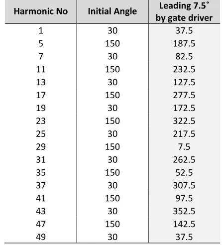
Table 2-1. Converter 1 output voltage phase shifting
Harmonic No Initial Angle Leading 7.5˚
by gate driver
1 30 37.5
5 150 187.5
7 30 82.5
11 150 232.5
13 30 127.5
17 150 277.5
19 30 172.5
23 150 322.5
25 30 217.5
29 150 7.5
31 30 262.5
35 150 52.5
37 30 307.5
41 150 97.5
43 30 352.5
47 150 142.5
49 30 37.5
Table 2-2. Converter 2 output voltage phase shifting
Harmonic No Initial Angle
Leading 172.5˚ by gate driver
Shift 180˚ using transformer
1 30 202.5 22.5
5 150 1012.5 112.5
7 30 1237.5 337.5
11 150 2047.5 67.5
13 30 2272.5 292.5
17 150 3082.5 22.5
19 30 3307.5 247.5
23 150 4117.5 337.5
25 30 4342.5 202.5
29 150 5152.5 292.5
31 30 5377.5 157.5
35 150 6187.5 247.5
37 30 6412.5 112.5
41 150 7222.5 202.5
43 30 7447.5 67.5
47 150 8257.5 157.5
Table 2-3. Converter 3 output voltage phase shifting
Harmonic No Initial Angle Leading 37.5˚
by gate driver
Lagging 30˚ using Aux. transformer
1 30 67.5 37.5
5 150 337.5 7.5
7 30 292.5 262.5
11 150 562.5 232.5
13 30 517.5 127.5
17 150 787.5 97.5
19 30 742.5 352.5
23 150 1012.5 322.5
25 30 967.5 217.5
29 150 1237.5 187.5
31 30 1192.5 82.5
35 150 1462.5 52.5
37 30 1417.5 307.5
41 150 1687.5 277.5
43 30 1642.5 172.5
47 150 1912.5 142.5
49 30 1867.5 37.5
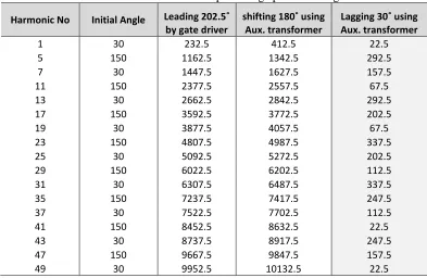
Table 2-4. Converter 4 output voltage phase shifting
Harmonic No Initial Angle Leading 202.5˚
by gate driver
shifting 180˚ using Aux. transformer
Lagging 30˚ using Aux. transformer
1 30 232.5 412.5 22.5
5 150 1162.5 1342.5 292.5
7 30 1447.5 1627.5 157.5
11 150 2377.5 2557.5 67.5
13 30 2662.5 2842.5 292.5
17 150 3592.5 3772.5 202.5
19 30 3877.5 4057.5 67.5
23 150 4807.5 4987.5 337.5
25 30 5092.5 5272.5 202.5
29 150 6022.5 6202.5 112.5
31 30 6307.5 6487.5 337.5
35 150 7237.5 7417.5 247.5
37 30 7522.5 7702.5 112.5
41 150 8452.5 8632.5 22.5
43 30 8737.5 8917.5 247.5
47 150 9667.5 9847.5 157.5
7.5˚
22.5˚
7.5˚
22.5˚
5th Harmonic
7.5˚ 7.5
22.5˚
7th Harmonic
22.5˚ 67.5˚
11th Harmonic
52.5˚
22.5˚
13th Harmonic
37.5˚
22.5˚ 17th Harmonic
7.5˚ 7.5˚
22.5˚
22.5˚
19th Harmonic
7.5˚
7.5˚
Figure 2-32.illustrative harmonic elimination of the 48-pulse inverter using the gate drive phase shift and also auxiliary and shunt transformers phase shifting. All the harmonics up to the 49th are illustrated. Blue, red, green, and black represent the NPC converter 1, 2, 3, and 4 respectively.
7.5˚ 29th Harmonic
22.5˚ 7.5˚
22.5˚
7.5˚
31st Harmonic
22.5˚ 7.5˚
22.5˚
35th Harmonic
52.5˚
67.5˚
37th
Harmonic
52.5˚ 22.5˚
41st Harmonic
7.5˚
22.5˚
7.5˚
22.5˚
43rd Harmonic
7.5˚ 67.5˚ 7.5˚
Chapter3: Dual Angle Control for Line-Frequency-Switched Static
Synchronous Compensators under System Faults
3. 1 Introduction
Despite the superior feature on voltage waveform quality and efficiency, the practical
angle-controlled STATCOMs suffer from the over-current (and trips) and possible saturation of the interfacing transformers caused by negative sequence current during unbalanced conditions and faults, when the VAR support is needed the most. It is important to note that solutions proposed in the literature to improve the PWM based VSC performance under unbalanced conditions are not applicable to angle-controlled STATCOMs. Angle-controlled
STATCOMs do not have the same degree of freedom as PWM-controlled STATCOM. The main motivation to use Angle-controlled STATCOM is to obtain higher waveform quality of voltage with lower losses compared to PWM VSC. This becomes especially important for utility application of large rated STATCOMs in the range of 100-150 MVA where standard PWM VSC for drives cannot be directly applied.
This chapter presents a new control structure for high power angle-controlled
STATCOMs during normal and fault conditions. As discussed earlier, the only control input in the angle-controlled STATCOM is phase angle difference between VSC and AC bus instantaneous voltage vector (α) [19]. In the proposed controller, α is split into two parts, αdc and αac .The DC part (αdc) which is the conventional angle-controller output is in charge of controlling the positive sequence VSC output voltage. The oscillating part (αac) controls the DC-link voltage oscillations with twice the line frequency to generate required fundamental negative sequence voltages at the VSC output terminals to limit the negative sequence current. Since this control scheme uses two angles (αdc and αac) as control inputs, it is called
without tripping.
In this chapter, we address the issue of limiting the STATCOM negative sequence current, and thus the resulting DC-link voltage oscillations, in high-power angle-controlled
STATCOMs, to enable the STATCOM to operate without tripping in the presence of power system faults and AC-system voltage unbalances. This is done by control action, which makes it unnecessary to constrain the design of STATCOM power components to achieve the same task. We give an analysis of STATCOM unbalanced operation, followed by a description of the proposed dual angle control method.
3. 2 Angle-controlled STATCOM under normal and system faults 3.2.1 Description of Conventional Angle-Controller Structure
The description of the angle-controlled STATCOM was presented in detail in the last chapter. To make this chapter self-sufficient a brief outline is also given in this chapter.All the VSCs, which are building block of FACTS devices, regardless of their topology can be divided into two types depending on their control methods. One type is vector controlled or PWM-based converter. The function of generating arbitrary voltage vector is already known for this type of inverters. This holds because the DC link voltage which is regulated to a constant reference value can be chopped with the PWM pulses to any arbitrary voltage vector with desired amplitude and angle. Figure 3-1indicates the control structure of a STATCOM working with vector controlled inverter. However, this type of inverter may be uneconomical for many transmission level FACTS devices due to the high switching losses of the PWM VSCs.
Figure 3-1.Control structure of a vector controlled (PWM) STATCOM.
Figure 3-2.Control structure of an angle-controlled STATCOM.
Figure 3-3.48-pulse inverter line to line output voltages.
based on the NYPA STATCOM (which was presented in the previous chapter) has been simulated in PSCAD/EMTDC. Voltage construction of this STACOM is carried out by a 48-pulse inverter as shown in Figure 3-3.Throughout this chapter, all the PSCAD/EMTDC simulation results, presented in different sections of this chapter are based on this STACOM simulation. The performance of this STATCOM under normal operating condition and variable instantaneous reactive current (iq) references is illustrated in Figure 3-4.
3.2.2 Angle-Controlled STATCOM under Unbalanced Conditions and System Faults
The VSC is the main building block of the STATCOM and many other converter-based FACTS devices. Therefore, the study on the methods to improve the VSC performance under unbalanced ac voltage condition is important and practical. Many different control structures have been proposed by the researchers to improve the VSC performance under fault conditions [36]- [54]. These are focused on mainly generating the current reference in both positive and negative synchronous frame to regulate the power or voltage at the point of common coupling (PCC). However, all these methods are based on controlling both the angle and magnitude of the VSC output voltage and are not applicable for angle-controlled
Figure 3-4.Angle-controlled STATCOM performance with two different instantaneous reactive current (Iq) references