Fusion global-local-topology particle swarm optimization for global optimization problems

Research Article

Fusion Global-Local-Topology Particle Swarm Optimization

for Global Optimization Problems

Zahra Beheshti, Siti Mariyam Shamsuddin, and Sarina Sulaiman

UTM Big Data Centre, Universiti Teknologi Malaysia, Skudai, 81310 Johor, Malaysia Correspondence should be addressed to Siti Mariyam Shamsuddin; [email protected]

Received 22 February 2014; Revised 18 May 2014; Accepted 24 May 2014; Published 25 June 2014

Academic Editor: Dan Simon

Copyright © 2014 Zahra Beheshti et al. This is an open access article distributed under the Creative Commons Attribution License, which permits unrestricted use, distribution, and reproduction in any medium, provided the original work is properly cited.

In recent years, particle swarm optimization (PSO) has been extensively applied in various optimization problems because of its structural and implementation simplicity. However, the PSO can sometimes find local optima or exhibit slow convergence speed when solving complex multimodal problems. To address these issues, an improved PSO scheme called fusion global-local-topology particle swarm optimization (FGLT-PSO) is proposed in this study. The algorithm employs both global and local topologies in PSO to jump out of the local optima. FGLT-PSO is evaluated using twenty (20) unimodal and multimodal nonlinear benchmark functions and its performance is compared with several well-known PSO algorithms. The experimental results showed that the proposed method improves the performance of PSO algorithm in terms of solution accuracy and convergence speed.

1. Introduction

PSO is a population-based metaheuristic algorithm intro-duced by Kennedy and Eberhart [1] in 1995. The algorithm imitates the social behavior of bird flocking or fish schooling to find the global best solution. Due to the simple concept, having a few parameters and being easy to implement, PSO has received much more attention to solve real-world opti-mization problems [2–6] in recent years. Nevertheless, PSO may easily get trapped in local optima when solving complex multimodal problems [7]. Hence, a number of variant PSO algorithms have been proposed in the literature to avoid the local optima and to find the best solution promptly.

The algorithm applies two different topologies to find a good solution: global and local topologies. In global topology, the position of each particle is affected by the best-fitness particles of the entire population in the search space while each particle is influenced by the best-fitness particles of its neighborhood in the local topology. Kennedy and Mendes proposed local (ring) topological structure PSO (LPSO) [8] and the Von Neumann topological structure PSO (VPSO) [9]. Mendes et al. [10] introduced the fully informed particle swarm (FIPS) algorithm and Ratnaweera et al. [11] suggested self-organizing hierarchical particle swarm optimizer with time-varying acceleration coefficients (HPSO-TVAC). Other

researchers presented the several variants of PSO algorithms such as dynamic multiswarm PSO (DMS-PSO) [12], com-prehensive learning PSO (CLPSO) [13], median-oriented particle swarm optimization (MPSO) [14], centripetal accel-erated particle swarm optimization (CAPSO) [15], quadratic interpolation PSO (QIPSO) [16], quantum-behaved particle swarm optimization (QPSO) [17], and adaptive particle swarm optimization (APSO) [18].

Although the aforementioned algorithms have obtained satisfactory results, there are still some disadvantages in their utilization. For example, LPSO presents a slow convergence rate in unimodal functions [14, 15] or CLPSO is not good for solving unimodal problems [13]. Moreover, some of the algorithms have a better performance than PSO but their structures are not as simple as PSO.

To overcome the disadvantages, this study introduces fusion global-local-topology particle swarm optimization (FGLT-PSO). The proposed algorithm performs a global search over the entire search space with a fast convergence speed using hybridizing two local and global topologies in PSO to jump out from local optima.

The remainder of this paper is organized as follows. In Section 2, a brief review of PSO is provided followed by some well-known PSO algorithms. The proposed algorithm Volume 2014, Article ID 907386, 19 pages

is described in Section 3 in detail. In Section 4, FGLT-PSO is used to solve several benchmark functions and its performance is compared with the other PSO algorithms in the literature. Finally, conclusions and the future research directions are presented inSection 5.

2. Particle Swarm Optimization (PSO)

2.1. PSO Framework. The PSO algorithm is a population-based metaheuristic algorithm that applies two approaches of global exploration and local exploitation to find the optimum solution. The exploration is the ability of expanding search space, where the exploitation is the ability of finding the optima around a good solution. The algorithm is initialized by creating a swarm, that is, population of particles, with ran-dom positions. Every particle is shown as a vector( ⃗𝑋_𝑖, ⃗𝑉_𝑖, ⃗𝑃_𝑖) in a 𝑑-dimensional search space where ⃗𝑋_𝑖 and ⃗𝑉_𝑖 are the position and velocity, respectively, and _𝑖⃗𝑃is the personal best position(𝑃best)found by the𝑖th particle:

⃗𝑋𝑖= (𝑥1𝑖, 𝑥2𝑖, . . . , 𝑥𝑑𝑖) for 𝑖 = 1, 2, . . . , 𝑁,

⃗𝑉

𝑖= (V1𝑖,V2𝑖, . . . ,V𝑑𝑖) for𝑖 = 1, 2, . . . , 𝑁,

⃗𝑃

𝑖= (𝑝𝑖1, 𝑝2𝑖, . . . , 𝑝𝑖𝑑) for 𝑖 = 1, 2, . . . , 𝑁.

(1)

In addition, the best position obtained by the entire popula-tion ( ⃗𝑃𝑔) is computed to update the particle velocity:

⃗𝑃𝑔 = (𝑝1

𝑔, 𝑝2𝑔, . . . , 𝑝𝑔𝑑) . (2)

Based on _𝑖⃗𝑃and ⃗𝑃𝑔, the next velocity and position of the𝑖th particle are computed using (3) and (4) as follows:

V_𝑖𝑑(𝑡 + 1) = 𝑤 ×V𝑑_𝑖 (𝑡) + 𝐶1×rand1× (𝑝𝑑𝑖 (𝑡) − 𝑥𝑑𝑖 (𝑡)) + 𝐶2

×rand₂× (𝑝_𝑔𝑑(𝑡) − 𝑥𝑑_𝑖 (𝑡)) ,

(3)

𝑥𝑑_𝑖 (𝑡 + 1) = 𝑥𝑑_𝑖 (𝑡) +V_𝑖𝑑(𝑡 + 1) , (4)

whereV𝑑_𝑖(𝑡 + 1)andV𝑑_𝑖(𝑡)are the next and current velocity of the𝑖th particle, respectively.𝑤is inertia weight,𝐶₁and𝐶₂ are acceleration coefficients, and rand₁and rand₂are random numbers in the interval[0, 1].𝑁is the number of particles; 𝑥𝑑

𝑖(𝑡+1)and𝑥𝑑𝑖(𝑡)are the next and current position of the𝑖th

particle.

Also, |V𝑑_𝑖(𝑡 + 1)| < V_max and V_max is set to a constant bounded based on the search space bound. A larger value of

wencourages global exploration (searching new areas), while a smaller value provides a local exploitation.

In (3), the second and the third terms are called cognition and social term, respectively. The two models applied to choose ⃗𝑃𝑔are known as𝑔best (for global topology) and𝑙best (for local topology) models. In this paper, the𝑔best model and𝑙best model are called PSO and LPSO, respectively.

2.2. Improved PSO Algorithms. Since Kennedy and Eberhart introduced PSO algorithm, the algorithm and its improved schemes have been extensively applied in many problems [20–25]. Many researchers have proposed the variants of modified PSO through swarm topology [8, 9], parameter selection [19,26], combining PSO with other evolutionary computation (EC) techniques [27,28], integration of its self-adaptation [29], and so on.

LPSO [8] and VPSO [9] were proposed based on a local topology to avoid premature convergence rate in solving multimodal problems. FIPS algorithm [10] is another PSO algorithm which uses the information of the entire neigh-borhood to guide the particles for finding the best solution. Dynamic multiswarm PSO (DMS-PSO) [12] was suggested by Liang and Suganthan to dynamically enhance the topo-logical structure. Ratnaweera et al. [11] proposed HPSO-TVAC algorithm based on linearly time-varying acceleration coefficients where a larger 𝐶₁ and a smaller 𝐶₂ are set at the beginning and gradually reversed throughout the search. Liang et al. [13] presented comprehensive learning particle swarm optimization (CLPSO) which focused on avoiding the local optima by encouraging each particle to learn its behavior from other particles on different dimensions.

In another research, a selection operator for PSO was first introduced by Angeline [30]. It is similar to what was used in a genetic algorithm (GA). Other researchers used a part of crossover [31] and mutation [29] operations from GA into PSO. Pant et al. proposed a quadratic crossover oper-ator to PSO algorithm called quadratic interpolation PSO (QIPSO) [16]. An adaptive fuzzy particle swarm optimization (AFPSO) [19] was proposed to utilize fuzzy inferences for adjusting acceleration coefficients. Meanwhile, the quadratic crossover operator [16] was used in the proposed AFPSO algorithm (AFPSO-QI) [19] to have better performance in solving multimodal problems. Zhan et al. presented an adaptive particle swarm optimization (APSO) [18] using a real-time evolutionary state estimation procedure and an elitist learning strategy. A variant of PSO algorithm based on orthogonal learning strategy (OLPSO) [32] was introduced to guide particles for discovering useful information from their personal best positions and from their neighborhood’s best position in order to fly in better directions. Gao et al. [33] used PSO with chaotic opposition-based population initialization and stochastic search technique to solve complex multimodal problems. The algorithm called CSPSO finds new solutions in the neighborhoods of the previous best positions in order to escape from local optima in multimodal functions. Beheshti et al. proposed median-oriented particle swarm optimization (MPSO) [14] and centripetal accelerated particle swarm optimization (CAPSO) [15] based on Newton’s laws of motion to accelerate the learning and convergence of optimization problems.

3. FGLT-PSO: The Proposed Method

→

Xi(t)

→

Pi(t)−

→

Xi(t)

→

Pi(t)

→

Vi(t)

→

Pgbest(t)−

→

Xi(t)

→

Pgbest(t)

→

Plbest(t)−

→

Xi(t)

→

Plbest(t)

→

Xi(t + 1)

C1(t)×rand₁×(Pi→ (t)−→Xi(t))

C2(t)×rand2×(

→

Plbest(t)−

→

Xi(t))

C3(t)×rand3×(

→

Pgbest(t)−

→

Xi(t))

w(t)×V→i(t)

Figure 1: Graphical representation of the particle movement using FGLT-PSO algorithm.

and LPSO illustrates good results in multimodal problems. Hence, both local and global topologies are hybridized in FGLT-PSO to increase the convergence rate and to avoid trapping into local optima.

In FGLT-PSO algorithm, each particle uses the best position found by its neighbors ( _𝑙⃗𝑃best) to update the particles’

velocities: ⃗𝑃

𝑙best= (𝑝_𝑙1best, 𝑝2𝑙best, . . . , 𝑝𝑙𝑑best) , (5) V𝑑_𝑖 (𝑡 + 1) = 𝑤 (𝑡) ×V𝑑_𝑖 (𝑡) + 𝐶₁(𝑡) ×rand₁

× (𝑝_𝑖𝑑(𝑡) − 𝑥𝑑_𝑖 (𝑡)) + 𝐶₂(𝑡) ×rand₂ × (𝑝_𝑙𝑑best(𝑡) − 𝑥𝑑𝑖 (𝑡)) .

(6)

The next position of each particle is computed based on the current position,𝑥𝑑_𝑖(𝑡), the next velocity,V𝑑_𝑖(𝑡 + 1), and the best position found by the swarm, _𝑔⃗𝑃best, as follows:

𝑥𝑑_𝑖 (𝑡 + 1) = 𝑥𝑑_𝑖 (𝑡) +V𝑑_𝑖 (𝑡 + 1) + 𝐶₃(𝑡) ×rand₃ × (𝑝_𝑔𝑑best(𝑡) − 𝑥𝑑𝑖 (𝑡)) ,

(7)

⃗𝑃

𝑔best= (𝑝1_𝑔best, 𝑝2𝑔best, . . . , 𝑝𝑑𝑔best) . (8)

In (6),𝑤is computed as

𝑤 (𝑡) = 𝑤max−𝑡 × (𝑤max_𝑇− 𝑤min). (9)

Also,𝐶₁(𝑡), 𝐶₂(𝑡), and𝐶₃(𝑡)are acceleration coefficients and modified according to (10):

𝐶_𝑗(𝑡) = 𝐶𝑗min+

𝑡 × (𝐶_𝑗max− 𝐶_𝑗min)

𝑇 , 𝑗 = 1, 2, 3, (10) where𝑡and𝑇are the current iteration and the number of maximum iterations, respectively.

The second term in (6) is called the cognition term, and the third terms in (6) and (7) are named the social terms. In (7),|𝑥𝑑_𝑖(𝑡 + 1)| < 𝑥_maxand𝑥_maxis set to a constant based on the search space bound.

3.2. Analysis of FGLT-PSO. A metaheuristic algorithm ex-plores new spaces to avoid trapping in a local optimum in the initial steps. Due to the poor exploration in the standard PSO (PSO), it can sometimes find local optima in multimodal problems. Sometimes, if a particle falls into a local optimum, it will not be able to get out of it. That is, if _𝑔⃗𝑃best obtained

through the population lies in a local optimum while the current position and the personal best position of particle𝑖 are in the same local optimum, the second and third terms of (3) tend to zero and 𝑤decreases linearly to near zero. Consequently, the next velocity of particle𝑖 tends to zero, and its next position in (4) does not change; thus, the particle remains in the local optimum. Hence, the main aim in FGLT-PSO is to overcome the poor exploration and to increase the convergence rate by combining the local and global searches as shown inFigure 1. The particles move in the search space based on the best solutions found by their neighbors ( _𝑙⃗𝑃best)

and the swarm ( _𝑔⃗𝑃best). At the beginning, the particles search

new spaces. By lapse of iterations, the exploration should fade out and the exploitation should fade in. It means the particles accelerate to the good solution and make search around it to find the best solution.

4. Experimental Results

Table 1: Dimensions, ranges, and global optimum values of test functions used in the experiments.

Test

function Dimension (𝑛) [Range]

𝑛 _𝑋

opt 𝐹opt

𝐹1(𝑥) 10/30/50 [−100, 100]𝑛 0 0

𝐹2(𝑥) 10/30/50 [−10, 10]𝑛 0 0

𝐹3(𝑥) 10/30/50 [−100, 100]𝑛 0 0

𝐹4(𝑥) 10/30/50 [−1.28, 1.28]𝑛 0 0

𝐹₅(𝑥) 10/30/50 [−10, 10]𝑛 1 0 𝐹₆(𝑥) 10/30/50 [−500, 500]𝑛 [420.96]𝑛 −418.9829 × 𝑛 𝐹₇(𝑥) 10/30/50 [−32, 32]𝑛 0 0 𝐹₈(𝑥) 10/30/50 [−50, 50]𝑛 0 0 𝐹9(𝑥) 10/30/50 [−5.12, 5.12]𝑛 0 0

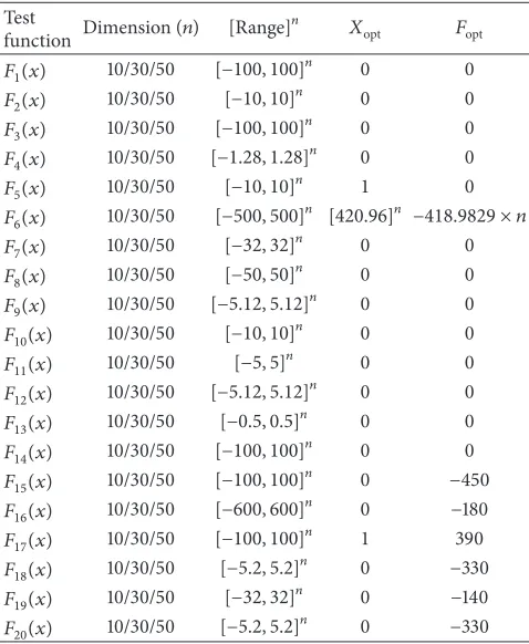
𝐹10(𝑥) 10/30/50 [−10, 10]𝑛 0 0

𝐹11(𝑥) 10/30/50 [−5, 5]𝑛 0 0

𝐹12(𝑥) 10/30/50 [−5.12, 5.12]𝑛 0 0

𝐹₁₃(𝑥) 10/30/50 [−0.5, 0.5]𝑛 0 0 𝐹₁₄(𝑥) 10/30/50 [−100, 100]𝑛 0 0 𝐹₁₅(𝑥) 10/30/50 [−100, 100]𝑛 0 −450 𝐹₁₆(𝑥) 10/30/50 [−600, 600]𝑛 0 −180 𝐹17(𝑥) 10/30/50 [−100, 100]𝑛 1 390

𝐹18(𝑥) 10/30/50 [−5.2, 5.2]𝑛 0 −330

𝐹19(𝑥) 10/30/50 [−32, 32]𝑛 0 −140

𝐹20(𝑥) 10/30/50 [−5.2, 5.2]𝑛 0 −330

4.1. Benchmark Functions. Twenty (20) minimization func-tions are applied in the experimental study including uni-modal, multiuni-modal, rotated, shifted, and shifted-rotated functions as detailed inTable 1. In the table,Range and 𝑛 are the feasible bound and the dimension of each func-tion, respectively. 𝐹opt is the optimum value of function.

Among the benchmarks, functions (1)–(5) are unimodal functions and functions(6)–(9)are in the class of multimodal functions. Functions (10)–(14) are rotated and functions (15)–(18) are shifted unimodal and multimodal functions. Two functions (19) and (20) are shifted-rotated multimodal functions.

In unimodal functions, the convergence rate of search algorithm is more interesting than the final results because other methods have been designed to optimize these kinds of functions. In multimodal functions, finding an optimal (or a good near-global optimal) solution is important. These functions are more difficult to optimize because the num-ber of local optima exponentially increases as the dimen-sion increases. Therefore, the search algorithms should not become trapped in a local optimum and should be able to obtain good solutions.

The rotation of function increases the function complex-ity. It does not affect the shape of function. The variable ⃗𝑌is computed using an orthogonal matrix𝑀[36] and applied to obtain the fitness value of rotated function as follows:

⃗𝑌 = 𝑀 × ⃗𝑋. (11)

In shifted functions, the global optimum𝑋∗⃗ = (𝑥∗₁, 𝑥₂∗, . . . , 𝑥∗

𝑛)is shifted to the new position ⃗𝑂 = (𝑜1, 𝑜2, . . . , 𝑜𝑛). All

the test functions are shown as follows.

(1) Sphere Model (unimodal function).Consider

𝐹₁(𝑥) =∑𝑛

𝑖=1

𝑥_𝑖2. (12)

(2) Shifted’s Schwefel’s Problem (unimodal function).Consider

𝐹2(𝑥) = 𝑛

∑

𝑖=1󵄨󵄨󵄨󵄨𝑥𝑖󵄨󵄨󵄨󵄨 + 𝑛

∏

𝑖=1󵄨󵄨󵄨󵄨𝑥𝑖󵄨󵄨󵄨󵄨. (13)

(3) Schwefel’s Problem 1.2 (unimodal function). Consider

𝐹₃(𝑥) =∑𝑛

𝑖=1

(∑𝑖

𝑗=1

𝑥_𝑗)

2

. (14)

(4) Quartic Function, That Is, Noise (unimodal function).

Consider

𝐹₄(𝑥) =∑𝑛

𝑖=1

𝑖𝑥4_𝑖 +random[0, 1) . (15)

(5) Rosenbrock’s Function (multimodal function).Consider

𝐹₅(𝑥) =𝑛−1∑

𝑖=1

[100(𝑥2_𝑖 − 𝑥_𝑖+1)2+ (𝑥_𝑖− 1)2] . (16)

𝐹₅ is unimodal in a 2-dimension or 3-dimension search space but can be treated as a multimodal function in high-dimensional cases.

(6) Generalized Schwefel’s Problem 2.26 (multimodal func-tion). Consider

𝐹₆(𝑥) =∑𝑛

𝑖=1

−𝑥_𝑖sin(√󵄨󵄨󵄨󵄨𝑥_𝑖󵄨󵄨󵄨󵄨). (17)

(7) Ackley’s Function (multimodal function). Consider

𝐹₇(𝑥) = −20exp(−0.2√1 𝑛

𝑛

∑

𝑖=1

𝑥2 𝑖)

−exp(1 𝑛

𝑛

∑

𝑖=1

cos2𝜋𝑥_𝑖) + 20 + 𝑒.

(18)

(8) Generalized Penalized Function (multimodal function). Consider

𝐹₈(𝑥) = 𝜋_𝑛{10sin(𝜋𝑦₁) +

𝑛−1

∑

𝑖=1

(𝑦_𝑖− 1)2

× [1 + 10sin2(𝜋𝑦_𝑖+1)] + (𝑦_𝑛− 1)2}

+∑𝑛

𝑖=1

Table 2: Minimization results for the unimodal and multimodal functions (maximum iteration = 5000 and𝑛 = 10).

Function FGLT-PSO PSO LPSO QIPSO

𝐹1

Avg. best solution 0.000e + 000 1.405e−135 1.452e−063 1.526e−138

SD 0.000e + 000 6.789e−135 5.681e−063 5.723e−138

Median best solution 0.000e+ 000 1.243e−139 7.381e−065 3.961e−142 Avg. iteration for finding the best solution 2646 5000 5000 5000

𝐹₂

Avg. best solution 2.741e−273 2.992e−077 4.130e−038 6.663e−079

SD 0.000e + 000 1.490e−076 7.564e−038 1.234e−078

Median best solution 6.578e−277 3.849e−079 9.945e−039 1.019e−079 Avg. iteration for finding the best solution 4952 5000 4999 5000

𝐹3

Avg. best solution 1.637e−116 3.215e−044 5.110e−014 3.919e−044

SD 8.969e−116 1.565e−043 1.126e−013 2.117e−043

Median best solution 2.369e−127 1.857e−048 5.320e−015 3.570e−048 Avg. iteration for finding the best solution 4630 4999 4999 4999

𝐹₄

Avg. best solution 3.209e−004 4.738e−004 1.269e−003 6.514e−004 SD 3.006e−004 2.057e−004 4.861e−004 3.241e−004 Median best solution 2.114e−004 4.595e−004 1.197e−003 5.797e−004 Avg. iteration for finding the best solution 3715 4404 4414 4459

𝐹5

Avg. best solution 2.973e−001 1.820e+ 000 1.661e+ 000 2.040e+ 000

SD 1.015e + 000 1.336e+ 000 1.281e+ 000 1.622e+ 000

Median best solution 4.614e−004 2.014e+ 000 1.727e+ 000 1.862e+ 000 Avg. iteration for finding the best solution 4537 4811 4988 4837

𝐹6

Avg. best solution −3.910e + 003 −3.452e+ 003 −3.892e+ 003 −3.424e+ 003

SD 1.184e + 002 2.307e+ 002 1.843e+ 002 2.775e+ 002

Median best solution −3.953e+ 003 −3.475e+ 003 −3.834e+ 003 −3.475e+ 003 Avg. iteration for finding the best solution 2974 2726 3918 2635

𝐹7

Avg. best solution 4.441e−015 4.322e−015 4.441e−015 4.441e−015

SD 0.000e + 000 6.486e−016 0.000e + 000 0.000e + 000

Median best solution 4.441e−015 4.441e−015 4.441e−015 4.441e−015 Avg. iteration for finding the best solution 376 3147 3772 3109

𝐹8

Avg. best solution 4.712e−032 4.712e−032 4.712e−032 4.712e−032

SD 1.670e−047 1.670e−047 1.670e−047 1.670e−047

Median best solution 4.712e−032 4.712e−032 4.712e−032 4.712e−032 Avg. iteration for finding the best solution 420 3166 3895 2687

𝐹9

Avg. best solution 9.495e−002 9.667e−001 1.574e+ 000 0.000e + 000 SD 2.720e−001 4.560e+ 000 1.065e+ 000 0.000e + 000 Median best solution 9.236e−008 0.000e+ 000 2.000e+ 000 0.000e+ 000 Avg. iteration for finding the best solution 4856 3357 4366 3401

Avg. rank 1.1 2.9 3.4 2.6

Final rank 1 3 4 2

Algorithms FGLT-PSO PSO LPSO QIPSO

𝑦_𝑖= 1 +𝑥𝑖+ 1

4 ,

𝑢 (𝑥_𝑖, 𝑎, 𝑘, 𝑚) ={{_{{ {

𝑘(𝑥_𝑖− 𝑎)𝑚 𝑥_𝑖> 𝑎

0 −𝑎 ≤ 𝑥𝑖≤ 𝑎

𝑘(−𝑥_𝑖− 𝑎)𝑚 𝑥_𝑖< −𝑎.

(19)

(9) Noncontinuous Rastrigin’s Function (multimodal function). Consider

𝐹₉(𝑥) =∑𝑛

𝑖=1

[𝑦_𝑖2− 10cos(2𝜋𝑦_𝑖) + 10] ,

where 𝑦_𝑖={_{ {

𝑥_𝑖 󵄨󵄨󵄨󵄨𝑥_𝑖󵄨󵄨󵄨󵄨 ≤ 0.5 round(2𝑥_𝑖)

2 󵄨󵄨󵄨󵄨𝑥𝑖󵄨󵄨󵄨󵄨 ≥ 0.5.

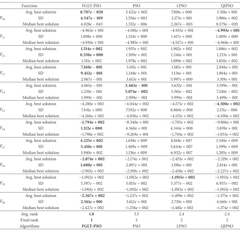
Table 3: Minimization results for the rotated and shifted unimodal and multimodal functions (maximum iteration = 5000 and𝑛 = 10).

Function FGLT-PSO PSO LPSO QIPSO

𝐹₁₀

Avg. best solution 7.056e−208 4.585e−059 2.358e−021 1.127e−058

SD 0.000e + 000 8.736e−059 7.425e−021 5.346e−058

Median best solution 1.930e−209 7.785e−060 3.417e−022 1.023e−060 Avg. iteration for finding the best solution 4741 4999 4997 4999

𝐹₁₁

Avg. best solution −6.602e +001 −6.645e + 001 −6.616e +001 −6.613e +001 SD 1.736e +000 1.175e + 000 9.989e−001 1.720e +000 Median best solution −6.606e +001 −6.614e +001 −6.607e +001 −6.588e +001 Avg. iteration for finding the best solution 3408 2930 3099 3185

𝐹12

Avg. best solution 1.604e + 001 2.352e +001 2.319e +001 2.278e +001

SD 2.974e + 000 3.762e +000 4.012e +000 4.387e +000

Median best solution 1.589e +001 2.358e +001 2.351e +001 2.240e +001 Avg. iteration for finding the best solution 2394 3656 3786 3660

𝐹13

Avg. best solution 0.000e + 000 1.351e +000 7.438e−008 7.957e−001

SD 0.000e + 000 3.079e +000 4.072e−007 2.428e +000

Median best solution 0.000e +000 0.000e +000 0.000e +000 0.000e +000 Avg. iteration for finding the best solution 448 3192 4877 3446

𝐹₁₄

Avg. best solution 1.165e−001 1.032e−001 9.987e−002 1.132e−001 SD 3.790e−002 1.826e−002 0.000e + 000 3.457e−002 Median best solution 9.987e−002 9.987e−002 9.987e−002 9.987e−002 Avg. iteration for finding the best solution 1998 2916 3268 2795

𝐹15

Avg. best solution −4.500e + 002 −4.396e +002 −4.480e +002 −4.406e +002

SD 8.039e−014 7.334e +000 2.470e +000 7.991e +000

Median best solution −4.500e +002 −4.450e +002 −4.500e +002 −4.450e +002 Avg. iteration for finding the best solution 1324 757 3561 1213

𝐹16

Avg. best solution −1.798e + 002 −1.745e +002 −1.793e +002 −1.766e +002

SD 3.789e−001 8.186e +000 5.222e−001 3.309e +000

Median best solution −1.800e +002 −1.780e +002 −1.789e +002 −1.780e +002 Avg. iteration for finding the best solution 2922 2592 3398 2711

𝐹₁₇

Avg. best solution 3.915e + 002 9.048e +006 6.752e +004 6.596e +006

SD 6.315e + 000 1.678e +007 3.676e +005 1.638e +007

Median best solution 3.900e +002 2.014e +006 3.933e +002 4.867e +002 Avg. iteration for finding the best solution 4831 3983 4884 4090

𝐹18

Avg. best solution −3.287e + 002 −3.215e +002 −3.247e +002 −3.233e +002

SD 1.113e + 000 5.979e +000 3.144e +000 4.822e +000

Median best solution −3.290e +002 −3.225e +002 −3.250e +002 −3.225e +002 Avg. iteration for finding the best solution 4809 3193 4509 3331

𝐹19

Avg. best solution −119.744 −119.745 −119.804 −119.746 SD 5.750e−002 7.142e−002 5.558e−002 6.911e−002 Median best solution −119.731 −119.748 −119.804 −119.73 Avg. iteration for finding the best solution 1849 2240 2072 2414

𝐹₂₀

Avg. best solution −3.196e + 002 −3.091e +002 −3.137e +002 −3.078e +002

SD 4.236e + 000 7.174e +000 5.338e +000 7.995e +000

Median best solution −3.196e +002 −3.102e +002 −3.130e +002 −3.079e +002 Avg. iteration for finding the best solution 3252 3315 4721 3479

Avg. rank 1.8 3.2 2.1 2.9

Final rank 1 4 2 3

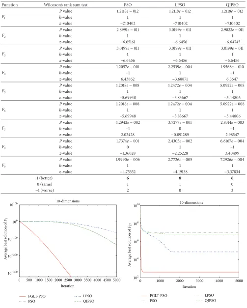
Table 4: Comparison of FGLT-PSO with PSO, LPSO, and QIPSO for the unimodal and multimodal functions using Wilcoxon’s rank sum test (𝑛 = 10).

Function Wilcoxon’s rank sum test PSO LPSO QIPSO

𝐹₁ 𝑃

value 1.2118e−012 1.2118e−012 1.2118e−012

ℎ-value 1 1 1

𝑧-value −7.10402 −7.10402 −7.10402

𝐹2

𝑃value 3.0199e−011 3.0199e−011 3.0199e−011

ℎ-value 1 1 1

𝑧-value −6.6456 −6.6456 −6.6456

𝐹₃ 𝑃

value 3.0199e−011 3.0199e−011 3.0199e−011

ℎ-value 1 1 1

𝑧-value −6.6456 −6.6456 −6.6456

𝐹₄ 𝑃

value 1.0576e−003 6.1210e−010 3.5923e−005

ℎ-value 1 1 1

𝑧-value −3.27475 −6.18728 −4.13225

𝐹5

𝑃value 1.5581e−008 1.8731e−007 1.0095e−008

ℎ-value 1 1 1

𝑧-value −5.65504 −5.21151 −5.72912

𝐹₆ 𝑃

value 6.3474e−011 1.2724e−001 9.3829e−010

ℎ-value 1 0 1

𝑧-value −6.53532 −1.52509 −6.11957

𝐹₇ 𝑃

value 3.3371e−001 — —

ℎ-value 0 0 0

𝑧-value 0.966667 — —

𝐹8

𝑃value — — —

ℎ-value 0 0 0

𝑧-value — — —

𝐹₉ 𝑃

value 1.9097e−005 1.6703e−006 6.2470e−010

ℎ-value −1 1 −1

𝑧-value 4.27519 −4.7897 6.18407

1 (better) 6 6 6

0 (same) 2 3 2

−1 (worse) 1 0 1

(10) Rotated Schwefel’s Problem 2.22 (unimodal function). Consider

𝐹₁₀(𝑥) =∑𝑛

𝑖=1󵄨󵄨󵄨󵄨𝑦𝑖󵄨󵄨󵄨󵄨 + 𝑛

∏

𝑖=1󵄨󵄨󵄨󵄨𝑦𝑖󵄨󵄨󵄨󵄨, 𝑦 = 𝑀 × 𝑥.

(21)

(11) Rotated 2𝑛 Minima Function (multimodal function).

Consider

𝐹₁₁(𝑥) =1 𝑛

𝑛

∑

𝑖=1

(𝑦_𝑖4− 16𝑦_𝑖2+ 5𝑦_𝑖) , 𝑦 = 𝑀 × 𝑥. (22)

(12) Rotated Rastrigin’s Function (multimodal function). Con-sider

𝐹₁₂(𝑥) =∑𝑛

𝑖=1

[𝑦2_𝑖 − 10cos(2𝜋𝑦_𝑖) + 10] , 𝑦 = 𝑀 × 𝑥. (23)

(13) Rotated Weierstrass’ Function (multimodal function). Consider

𝐹₁₃(𝑥) =∑𝑛

𝑖=1

(𝑘∑max

𝑘=0

[𝑎𝑘cos(2𝜋𝑏𝑘(𝑦_𝑖+ 0.5))])

− 𝑛𝑘∑max

𝑘=0

[𝑎𝑘cos(2𝜋𝑏𝑘× 0.5)] ,

𝑦 = 𝑀 × 𝑥, 𝑎 = 0.5, 𝑏 = 3, 𝑘max= 20.

(24)

(14) Rotated Salomon’s Function (multimodal function). Con-sider

𝐹₁₄(𝑥) = 1 −cos(2𝜋√

𝑛

∑

𝑖=1

𝑦2

𝑖) + 0.1√ 𝑛

∑

𝑖=1

𝑦2

𝑖, 𝑦 = 𝑀 × 𝑥.

Table 5: Comparison of FGLT-PSO with PSO, LPSO, and QIPSO for the rotated and shifted unimodal and multimodal functions using Wilcoxon’s rank sum test (𝑛 = 10).

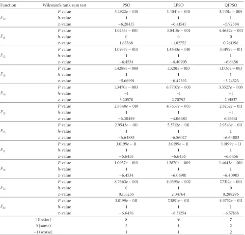
Function Wilcoxon’s rank sum test PSO LPSO QIPSO

𝐹₁₀ 𝑃

value 3.0199e−011 3.0199e−011 3.0199e−011

ℎ-value 1 1 1

𝑧-value −6.6456 −6.6456 −6.6456

𝐹11

𝑃value 4.1191e−001 7.3940e−001 8.4180e−001

ℎ-value 0 0 0

𝑧-value 0.820536 0.33265 0.19959

𝐹₁₂ 𝑃

value 1.8567e−009 1.8500e−008 5.5329e−008

ℎ-value 1 1 1

𝑧-value −6.00987 −5.62547 −5.43328

𝐹₁₃ 𝑃

value 2.1577e−002 2.1577e−002 8.1523e−002

ℎ-value 1 1 0

𝑧-value −2.29773 −2.29773 −1.74192

𝐹14

𝑃value 1.1439e−001 1.4425e−004 7.7181e−001

ℎ-value 0 −1 0

𝑧-value 1.57878 3.80076 0.290007

𝐹₁₅ 𝑃

value 1.5553e−011 1.2883e−011 1.7966e−008

ℎ-value 1 1 1

𝑧-value −6.74264 −6.76995 −5.63053

𝐹₁₆ 𝑃

value 1.2755e−010 1.9667e−003 5.5338e−010

ℎ-value 1 1 1

𝑧-value −6.43006 −3.09521 −6.20317

𝐹17

𝑃value 7.3270e−011 3.6443e−008 5.0030e−010

ℎ-value 1 1 1

𝑧-value −6.51381 −5.50727 −6.21901

𝐹₁₈ 𝑃

value 5.7512e−006 3.5043e−007 4.0269e−005

ℎ-value 1 1 1

𝑧-value −4.53533 −5.09408 −4.10593

𝐹19

𝑃value 9.2344e−001 2.3885e−004 8.6499e−001

ℎ-value 0 −1 0

𝑧-value 0.0960988 3.67393 0.170021

𝐹20

𝑃value 5.2991e−008 9.2051e−005 4.6756e−008

ℎ-value 1 1 1

𝑧-value −5.44097 −3.91064 −5.46322

1 (better) 8 8 7

0 (same) 3 1 4

−1 (worse) 0 2 0

(15) Shifted Schwefel’s Problem 2.21 (unimodal function). Con-sider

𝐹₁₅(𝑥) =max_𝑖{󵄨󵄨󵄨󵄨𝑧_𝑖󵄨󵄨󵄨󵄨, 1 ≤ 𝑖 ≤ 𝑛} + 𝑓bias₁₅,

𝑓bias₁₅= −450, 𝑧 = 𝑥 − 𝑜. (26)

(16) Shifted Generalized Griewank’s Function (multimodal function). Consider

𝐹₁₆(𝑥) = ₄₀₀₀1 ∑𝑛

𝑖=1

𝑧_𝑖2−∏𝑛

𝑖=1

cos(𝑧𝑖

√𝑖) + 1 + 𝑓bias16,

𝑓bias₁₆= −180, 𝑧 = 𝑥 − 𝑜. (27)

(17) Shifted Rosenbrock’s Function (multimodal function). Consider

𝐹₁₇(𝑥) =𝑛−1∑

𝑖=1

[100(𝑧2_𝑖 − 𝑧_𝑖+1)2+ (𝑧_𝑖− 1)2] + 𝑓bias₁₇,

𝑓bias₁₇= 390, 𝑧 = 𝑥 − 𝑜 + 1. (28)

(18) Shifted Rastrigin’s Function (multimodal function). Con-sider

𝐹₁₈(𝑥) =∑𝑛

𝑖=1

[𝑧2_𝑖 − 10cos(2𝜋𝑧_𝑖) + 10] + 𝑓bias₁₈,

𝑓bias₁₈= −330, 𝑧 = 𝑥 − 𝑜.

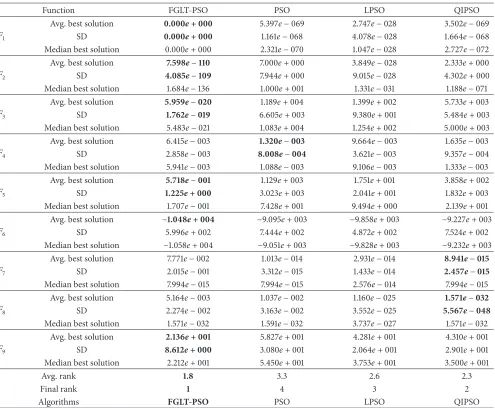
Table 6: Minimization results for the unimodal and multimodal functions (maximum iteration = 10000 and𝑛 = 30).

Function FGLT-PSO PSO LPSO QIPSO

𝐹₁

Avg. best solution 0.000e + 000 5.397e−069 2.747e−028 3.502e−069

SD 0.000e + 000 1.161e−068 4.078e−028 1.664e−068

Median best solution 0.000e +000 2.321e−070 1.047e−028 2.727e−072

𝐹2

Avg. best solution 7.598e−110 7.000e +000 3.849e−028 2.333e +000

SD 4.085e−109 7.944e +000 9.015e−028 4.302e +000

Median best solution 1.684e−136 1.000e +001 1.331e−031 1.188e−071

𝐹3

Avg. best solution 5.959e−020 1.189e +004 1.399e +002 5.733e +003

SD 1.762e−019 6.605e +003 9.380e +001 5.484e +003

Median best solution 5.483e−021 1.083e +004 1.254e +002 5.000e +003

𝐹4

Avg. best solution 6.415e−003 1.320e−003 9.664e−003 1.635e−003 SD 2.858e−003 8.008e−004 3.621e−003 9.357e−004 Median best solution 5.941e−003 1.088e−003 9.106e−003 1.333e−003

𝐹₅

Avg. best solution 5.718e−001 1.129e +003 1.751e +001 3.858e +002

SD 1.225e + 000 3.023e +003 2.041e +001 1.832e +003

Median best solution 1.707e−001 7.428e +001 9.494e +000 2.139e +001

𝐹6

Avg. best solution −1.048e + 004 −9.095e +003 −9.858e +003 −9.227e +003 SD 5.996e +002 7.444e +002 4.872e +002 7.524e +002 Median best solution −1.058e +004 −9.051e +003 −9.828e +003 −9.232e +003

𝐹7

Avg. best solution 7.771e−002 1.013e−014 2.931e−014 8.941e−015 SD 2.015e−001 3.312e−015 1.433e−014 2.457e−015 Median best solution 7.994e−015 7.994e−015 2.576e−014 7.994e−015

𝐹₈

Avg. best solution 5.164e−003 1.037e−002 1.160e−025 1.571e−032 SD 2.274e−002 3.163e−002 3.552e−025 5.567e−048 Median best solution 1.571e−032 1.591e−032 3.737e−027 1.571e−032

𝐹₉

Avg. best solution 2.136e + 001 5.827e +001 4.281e +001 4.310e +001

SD 8.612e + 000 3.080e +001 2.064e +001 2.901e +001

Median best solution 2.212e +001 5.450e +001 3.753e +001 3.500e +001

Avg. rank 1.8 3.3 2.6 2.3

Final rank 1 4 3 2

Algorithms FGLT-PSO PSO LPSO QIPSO

(19) Shifted Rotated Ackley’s Function (multimodal function). Consider

𝐹₁₉(𝑥) = −20exp(−0.2√1 𝑛

𝑛

∑

𝑖=1

𝑧2 𝑖)

−exp(1 𝑛

𝑛

∑

𝑖=1

cos2𝜋𝑧_𝑖) + 20 + 𝑒 + 𝑓bias₁₉, (30)

where 𝑓bias₁₉ = −140; 𝑧 = (𝑥 − 𝑜) × 𝑀󸀠 is a linear transformation matrix with condition number = 100.

(20) Shifted Rotated Rastrigin’s Function (multimodal func-tion). Consider

𝐹₂₀(𝑥) =∑𝑛

𝑖=1

[𝑧_𝑖2− 10cos(2𝜋𝑧_𝑖) + 10] + 𝑓bias₂₀, (31)

where 𝑓bias₂₀ = −330; 𝑧 = (𝑥 − 𝑜) × 𝑀󸀠 is a linear transformation matrix with condition number = 2.

4.2. Results of FGLT-PSO. The results of FGLT-PSO are provided in three sections. InSection 4.2.1, the acceleration coefficients 𝐶₁, 𝐶₂, and 𝐶₃ in the proposed method are changed according to (10) and inSection 4.2.2, these factors are constant. In these sections, FGLT-PSO is evaluated using the benchmark functions with dimensions 10, 30, and 50. The number of maximum iterations is set at 5000 for𝑛 = 10, at 10000 for𝑛 = 30, and at 15000 for𝑛 = 50. The population size is set to 50 (𝑁 = 50). Also,𝑤decreases linearly from 0.9 to 0.4.

InSection 4.2.3, the results of FGLT-PSO are compared with those of several well-known PSO algorithms from [19] on the common functions. In this section, the population size is set to 30 (𝑁 = 30),𝑛is 30, and the number of maximum iterations is set at 10000.

Table 7: Minimization results for the rotated and shifted unimodal and multimodal functions (maximum iteration = 10000 and𝑛 = 30).

Function FGLT-PSO PSO LPSO QIPSO

𝐹10

Avg. best solution 8.707e−020 3.422e+ 002 7.818e+ 000 5.318e+ 001

SD 4.547e−019 1.556e+ 003 2.173e+ 001 1.986e+ 002

Median best solution 4.028e−043 1.332e−006 2.267e−003 8.579e−020

𝐹₁₁

Avg. best solution −4.963e+ 001 −4.981e+ 001 −4.933e+ 001 −4.993e + 001 SD 1.098e+ 000 1.324e+ 000 1.417e+ 000 1.489e+ 000 Median best solution −4.930e+ 001 −4.985e+ 001 −4.927e+ 001 −4.968e+ 001

𝐹12

Avg. best solution 1.514e + 002 1.935e+ 002 1.902e+ 002 1.886e+ 002

SD 8.330e + 000 1.509e+ 001 1.246e+ 001 1.233e+ 001

Median best solution 1.511e+ 002 1.978e+ 002 1.899e+ 002 1.850e+ 002

𝐹₁₃

Avg. best solution 7.160e−001 3.101e+ 001 1.185e+ 001 2.046e+ 001

SD 9.412e−001 1.248e+ 001 1.136e+ 001 1.804e+ 001

Median best solution 2.067e−001 3.613e+ 001 5.997e+ 000 3.319e+ 001

𝐹₁₄

Avg. best solution 4.065e−001 3.465e−001 3.632e−001 3.599e−001 SD 1.230e−001 5.074e−002 5.561e−002 7.240e−002 Median best solution 3.999e−001 2.999e−001 3.999e−001 3.499e−001

𝐹15

Avg. best solution −4.280e+ 002 −4.044e+ 002 −4.175e+ 002 −4.500e + 002 SD 7.441e+ 000 7.592e+ 000 8.860e+ 000 2.151e−006 Median best solution −4.266e+ 002 −4.056e+ 002 −4.155e+ 002 −4.500e+ 002

𝐹₁₆

Avg. best solution −1.794e + 002 −8.340e+ 001 −1.705e+ 002 −9.806e+ 001

SD 1.112e + 000 4.560e+ 001 4.344e+ 000 3.839e+ 001

Median best solution −1.798e+ 002 −9.269e+ 001 −1.704e+ 002 −1.053e+ 002

𝐹17

Avg. best solution 4.225e + 002 1.658e+ 009 8.168e+ 007 1.549e+ 009

SD 5.410e + 001 1.409e+ 009 5.644e+ 007 1.599e+ 009

Median best solution 3.940e+ 002 1.136e+ 009 6.932e+ 007 1.205e+ 009

𝐹18

Avg. best solution −2.874e + 002 −2.174e+ 002 −2.455e+ 002 −2.219e+ 002

SD 1.680e + 001 2.897e+ 001 1.196e+ 001 2.614e+ 001

Median best solution −2.902e+ 002 −2.199e+ 002 −2.458e+ 002 −2.227e+ 002

𝐹₁₉

Avg. best solution −1.1912e+ 002 −1.1912e+ 002 −1.1915e + 002 −1.1913e+ 002 SD 5.597e−002 5.015e−002 5.377e−002 6.957e−002 Median best solution −1.1911e+ 002 −1.1911e+ 002 −1.1915e+ 002 −1.1913e+ 002

𝐹20

Avg. best solution −2.367e + 002 −1.237e+ 002 −1.499e+ 002 −1.375e+ 002

SD 2.561e + 001 3.612e+ 001 2.719e+ 001 4.160e+ 001

Median best solution −2.427e+ 002 −1.256e+ 002 −1.481e+ 002 −1.374e+ 002

Avg. rank 1.8 3.5 2.4 2.4

Final rank 1 3 2 2

Algorithms FGLT-PSO PSO LPSO QIPSO

4.2.1. The Results of Proposed Method with Variable Accelera-tion Coefficients. Four algorithms of FGLT-PSO, PSO, LPSO, and QIPSO are randomly initialized and run on benchmark functions. The average best solution, the standard deviation (SD), and the median of the best solution in the last iteration are reported in Tables2, 3,6,7,10, and11. The best results from among the algorithms are shown in bold numbers. In the tables, the algorithms are ranked based on the average best results.

Moreover, Wilcoxon’s rank sum test [37] is conducted in order to determine whether the results obtained by the FGLT-PSO are different from those generated by other algorithms with a statistical significance. The tests are shown in Tables 4, 5, 8, 9, 12, and13, where ℎ-value = 1 indicates the case

in which proposed algorithm significantly outperformed the compared algorithm with 95% certainty, ℎ-value = −1 represents that the compared algorithm is significantly better than the proposed algorithm, andℎ-value = 0 denotes that the results of the two considered algorithms are not significantly different. In these tables, rows 1 (better), 0 (same), and −1 (worse) give the number of functions that the FGLT-PSO performs significantly better than, almost the same as, and significantly worse than the compared algorithm, respectively.

Table 8: Comparison of FGLT-PSO with PSO, LPSO, and QIPSO for the unimodal and multimodal functions using Wilcoxon’s rank sum test (𝑛 = 30).

Function Wilcoxon’s rank sum test PSO LPSO QIPSO

𝐹₁ 𝑃

value 1.2118e−012 1.2118e−012 1.2118e−012

ℎ-value 1 1 1

𝑧-value −7.10402 −7.10402 −7.10402

𝐹2

𝑃value 2.8991e−011 3.0199e−011 2.9822e−011

ℎ-value 1 1 1

𝑧-value −6.65161 −6.6456 −6.64745

𝐹₃ 𝑃

value 3.0199e−011 3.0199e−011 3.0199e−011

ℎ-value 1 1 1

𝑧-value −6.6456 −6.6456 −6.6456

𝐹4

𝑃value 1.2057e−010 2.2539e−004 1.9568e−010

ℎ-value −1 1 −1

𝑧-value 6.43862 −3.68871 6.3647

𝐹5

𝑃value 1.2018e−008 1.2472e−004 5.0922e−008

ℎ-value 1 1 1

𝑧-value −5.69948 −3.83667 −5.44806

𝐹₆ 𝑃

value 1.2018e−008 1.2472e−004 5.0922e−008

ℎ-value 1 1 1

𝑧-value −5.69948 −3.83667 −5.44806

𝐹7

𝑃value 4.2942e−002 3.7277e−001 2.8314e−003

ℎ-value −1 0 −1

𝑧-value 2.02428 −0.891289 2.98547

𝐹8

𝑃value 1.7374e−001 2.4305e−002 6.6167e−004

ℎ-value 0 1 −1

𝑧-value −1.36028 −2.25228 3.40499

𝐹₉ 𝑃

value 1.9990e−006 2.7726e−005 7.2926e−004

ℎ-value 1 1 1

𝑧-value −4.75352 −4.19138 −3.37834

1 (better) 6 8 6

0 (same) 1 1 0

−1 (worse) 2 0 3

0 500 1000 1500 2000 2500 3000 3500 4000 4500 5000

10-dimensions _{10-dimensions}

FGLT-PSO PSO

LPSO QIPSO

FGLT-PSO PSO

LPSO QIPSO Iteration

0 1000 2000 3000 4000 5000

Iteration 10−300

10−200

10−100

100

10100

102

104

106

108

1010

A

verag

e b

est s

o

lu

tio

n o

f

F1

A

verag

e b

est s

o

lu

tio

n o

f

F17

Table 9: Comparison of FGLT-PSO with PSO, LPSO, and QIPSO for the rotated and shifted unimodal and multimodal functions using Wilcoxon’s rank sum test (𝑛 = 30).

Function Wilcoxon’s rank sum test PSO LPSO QIPSO

𝐹₁₀ 𝑃

value 3.2922e−010 1.4041e−010 3.1451e−009

ℎ-value 1 1 1

𝑧-value −6.28435 −6.41545 −5.92384

𝐹11

𝑃value 1.0233e−001 3.0418e−001 4.4642e−001

ℎ-value 0 0 0

𝑧-value 1.63368 −1.02752 0.761398

𝐹₁₂ 𝑃

value 1.0937e−010 1.4643e−010 3.0199e−011

ℎ-value 1 1 1

𝑧-value −6.4534 −6.40905 −6.6456

𝐹₁₃ 𝑃

value 1.4288e−008 1.3281e−010 1.1736e−003

ℎ-value 1 1 1

𝑧-value −5.66991 −6.42392 −3.24523

𝐹14

𝑃value 1.3470e−003 6.7707e−003 3.5527e−003

ℎ-value −1 −1 −1

𝑧-value 3.20578 2.70792 2.91537

𝐹₁₅ 𝑃

value 2.8840e−010 4.7657e−005 2.8252e−011

ℎ-value 1 1 −1

𝑧-value −6.30489 −4.06683 6.65541

𝐹₁₆ 𝑃

value 2.9543e−011 5.3712e−011 2.9543e−011

ℎ-value 1 1 1

𝑧-value −6.64883 −6.56027 −6.64883

𝐹17

𝑃value 3.0199e−11 3.0199e−11 3.0199e−11

ℎ-value 1 1 1

𝑧-value −6.6456 −6.6456 −6.6456

𝐹₁₈ 𝑃

value 1.0937e−010 1.2870e−009 1.4643e−010

ℎ-value 1 1 1

𝑧-value −6.4534 −6.06901 −6.40905

𝐹₁₉ 𝑃

value 8.7663e−001 4.0595e−002 7.7312e−001

ℎ-value 0 1 0

𝑧-value 0.155236 2.04764 0.288296

𝐹20

𝑃value 3.0199e−011 7.3891e−011 4.9752e−011

ℎ-value 1 1 1

𝑧-value −6.6456 −6.51254 −6.57168

1 (better) 8 9 7

0 (same) 2 1 2

−1 (worse) 1 1 2

In these tables, the benchmark functions are divided to two categories:(1)unimodal and multimodal functions and (2)rotated, shifted, and shifted-rotated unimodal and multimodal functions. The experimental results demonstrate that FGLT-PSO performs superior results for most of the functions in all tested dimensions.

Tables 2 and 3 show the experimental results for all benchmark functions with dimension𝑛 = 10. As illustrated, the FGLT-PSO algorithm surpasses the PSO, LPSO, and QIPSO algorithms in minimizing functions (1)–(6), (10), (12), (13), (15)–(18), and (20). Moreover, the proposed method provides significant improvements in functions(1), (2), (3), (10), (13), (17), and (18). In these functions, the

Table 10: Minimization results for the unimodal and multimodal functions (maximum iteration = 15000 and𝑛 = 50).

Function FGLT-PSO PSO LPSO QIPSO

𝐹1

Avg. best solution 5.239e−232 7.5857e−049 7.297e−020 2.446e−049

SD 0.000e + 000 2.1243e−048 7.695e−020 8.478e−049

Median best solution 2.541e−251 4.5415e−050 4.843e−020 1.395e−050

𝐹2

Avg. best solution 9.246e−075 3.400e +001 2.194e−015 1.367e +001

SD 3.646e−074 1.714e +001 1.439e−015 1.159e +001

Median best solution 2.684e−080 3.000e +001 1.881e−015 1.000e +001

𝐹₃

Avg. best solution 1.098e−008 4.167e +004 2.775e +004 3.585e +004

SD 2.405e−008 1.404e +004 8.532e +003 1.967e +004

Median best solution 5.928e−009 4.002e +004 2.859e +004 3.434e +004

𝐹4

Avg. best solution 5.070e−002 6.015e +000 6.452e−002 2.055e−002 SD 2.802e−002 5.352e +000 1.488e−002 4.363e−003 Median best solution 4.205e−002 5.385e +000 6.409e−002 1.971e−002

𝐹₅

Avg. best solution 6.128e + 000 1.568e +003 6.024e +001 4.700e +002

SD 5.716e + 000 3.409e +003 3.032e +001 1.817e +003

Median best solution 5.080e +000 8.179e +001 7.397e +001 7.942e +001

𝐹₆

Avg. best solution −1.505e + 004 −1.364e +004 −1.470e +004 −1.339e +004 SD 9.481e +002 9.581e +002 8.491e +002 1.025e +003 Median best solution −1.515e +004 −1.349e +004 −1.445e +004 −1.343e +004

𝐹7

Avg. best solution 1.299e +000 2.049e +000 1.145e−005 1.782e−014 SD 5.560e−001 4.661e +000 6.223e−005 3.695e−015 Median best solution 1.282e +000 2.220e−014 1.782e−009 1.510e−014

𝐹₈

Avg. best solution 1.061e−001 1.451e−002 3.831e−012 2.074e−003 SD 1.935e−001 3.535e−002 1.984e−011 1.136e−002 Median best solution 2.081e−005 1.308e−032 2.881e−015 9.423e−033

𝐹₉

Avg. best solution 4.759e + 001 1.980e +002 1.872e +002 1.546e +002

SD 2.294e + 001 4.888e +001 3.958e +001 5.192e +001

Median best solution 4.636e +001 1.890e +002 1.850e +002 1.475e +002

Avg. rank 1.7 3.7 2.3 2.3

Final rank 1 3 2 2

Algorithms FGLT-PSO PSO LPSO QIPSO

0 2000 4000 6000 8000 10000

Iteration

30-dimensions 30-dimensions

0 2000 4000 6000 8000 10000

0 50 100

Iteration

FPSO PSO

LPSO QIPSO

FPSO PSO

LPSO QIPSO 10−20

10−15

10−10

10−5

100

105

1010

−100 −50

−150

−200

−250

−300

A

verag

e b

est s

o

lu

tio

n o

f

F3

A

verag

e b

es

t s

o

lu

tio

n o

f

F18

Table 11: Minimization results for the rotated and shifted unimodal and multimodal functions (maximum iteration = 15000 and𝑛 = 50).

Function FGLT-PSO PSO LPSO QIPSO

𝐹10

Avg. best solution 9.936e−031 6.202e +009 5.150e +003 3.989e +006

SD 5.442e−030 2.576e +010 1.153e +004 1.825e +007

Median best solution 1.121e−048 1.763e +005 1.184e +002 5.637e−007

𝐹₁₁

Avg. best solution −4.401e + 001 −4.328e +001 −4.357e +001 −4.385e +001

SD 1.043e + 000 1.331e +000 9.431e−001 1.329e +000

Median best solution −4.391e +001 −4.344e +001 −4.339e +001 −4.367e +001

𝐹12

Avg. best solution 3.155e + 002 4.234e +002 3.995e +002 4.045e +002

SD 1.166e + 001 3.689e +001 1.813e +001 2.468e +001

Median best solution 3.171e +002 4.236e +002 3.995e +002 4.062e +002

𝐹₁₃

Avg. best solution 1.660e + 001 6.640e +001 5.210e +001 4.946e +001

SD 6.875e + 000 2.371e +000 1.517e +001 2.599e +001

Median best solution 1.759e +001 6.697e +001 6.163e +001 6.361e +001

𝐹₁₄

Avg. best solution 7.599e−001 5.899e−001 8.067e−001 6.099e−001 SD 3.103e−001 8.030e−002 9.046e−002 8.847e−002 Median best solution 6.999e−001 5.999e−001 7.999e−001 5.999e−001

𝐹15

Avg. best solution −3.976e +002 −3.795e +002 −4.019e +002 −4.499e + 002 SD 5.964e +000 1.974e +001 6.096e +000 1.849e−003 Median best solution −3.974e +002 −3.815e +002 −4.021e +002 −4.50e +002

𝐹₁₆

Avg. best solution −1.791e + 002 8.313e +001 −1.551e +002 6.894e +001

SD 1.212e + 000 9.121e +001 1.216e +001 7.896e +001

Median best solution −1.797e +002 7.911e +001 −1.565e +002 7.481e +001

𝐹17

Avg. best solution 4.260e + 002 8.648e +009 3.341e +008 8.196e +009

SD 7.188e + 001 4.442e +009 2.597e +008 5.588e +009

Median best solution 3.977e +002 8.332e +009 2.599e +008 6.614e +009

𝐹18

Avg. best solution −1.920e + 002 −4.497e +001 −9.832e +001 −3.612e +001

SD 2.634e + 001 4.206e +001 1.963e +001 4.934e +001

Median best solution −1.944e +002 −4.804e +001 −9.679e +001 −2.665e +001

𝐹₁₉

Avg. best solution −1.189e +002 −1.189e +002 −1.190e + 002 −1.189e +002 SD 4.303e−002 4.364e−002 5.121e−002 5.576e−002 Median best solution −1.189e +002 −1.189e +002 −1.190e +002 −1.189e +002

𝐹20

Avg. best solution −1.016e + 002 1.537e +002 5.974e +001 1.082e +002

SD 4.898e + 001 8.906e +001 5.117e +001 9.020e +001

Median best solution −1.004e +002 1.539e +002 6.594e +001 1.035e +002

Avg. rank 1.5 3.6 2.3 2.7

Final rank 1 4 2 3

Algorithms FGLT-PSO PSO LPSO QIPSO

Figure 2. The results in this figure illustrate that FGLT-PSO tends to find the global optimum in𝐹₁and 𝐹₁₇ faster than PSO, LPSO, and QIPSO and obtains the highest accuracy for these functions from among all the algorithms.

The minimization results of the benchmark functions with dimension 𝑛 = 30 are presented in Tables 6 and 7. As seen in these tables and Tables8 and 9, the FGLT-PSO outperforms the FGLT-PSO, LFGLT-PSO, and QIFGLT-PSO algorithms in functions(1),(2),(3),(5),(6),(9),(10),(12),(13),(16),(17), (18), and(20). The largest difference in performance between the proposed algorithm with PSO, LPSO, and QIPSO occurs for the functions(1),(2),(3),(5),(16),(17),(18), and(20). Figure 3illustrates the progress of the average best solution over 30 runs for𝐹₃and𝐹₁₈. As demonstrated, the FGLT-PSO shows a higher convergence rate than the other algorithms.

Tables10and11present the results of algorithms for the test functions with dimension𝑛 = 50. As illustrated in these tables and regarding the results of Wilcoxon’s rank sum in Tables12and13, the performance of proposed method is the best in most of the functions especially for functions(1),(2), (3), (5),(6),(9),(10), (11), (12),(13), (16), (17),(18), and (20). The superior convergence rate of FGLT-PSO is shown inFigure 4. The results in this figure show that the FGLT-PSO performs the best for the test functions𝐹₁₆and𝐹₂₀with 𝑛 = 50.

Table 12: Comparison of FGLT-PSO with PSO, LPSO, and QIPSO for the unimodal and multimodal functions using Wilcoxon’s rank sum test (𝑛 = 50).

Function Wilcoxon’s rank sum test PSO LPSO QIPSO

𝐹1

𝑃value 3.0199e−011 3.0199e−011 3.0199e−011

ℎ-value 1 1 1

𝑧-value −6.6456 −6.6456 −6.6456

𝐹₂ 𝑃

value 2.9673e−011 3.0199e−011 2.9229e−011

ℎ-value 1 1 1

𝑧-value −6.64819 −6.6456 −6.65041

𝐹3

𝑃value 3.0199e−011 3.0199e−011 3.0199e−011

ℎ-value 1 1 1

𝑧-value −6.6456 −6.6456 −6.6456

𝐹₄ 𝑃

value 2.5306e−004 3.9881e−004 3.1589e−010

ℎ-value 1 1 −1

𝑧-value −3.65915 −3.54087 6.29077

𝐹₅ 𝑃

value 6.1210e−010 9.7555e−010 1.2870e−009

ℎ-value 1 1 1

𝑧-value −6.18728 −6.11336 −6.06901

𝐹6

𝑃value 2.8790e−006 9.3341e−002 2.5711e−007

ℎ-value 1 0 1

𝑧-value −4.67927 −1.67803 −5.15244

𝐹₇ 𝑃

value 7.7050e−006 3.0199e−011 1.4811e−011

ℎ-value −1 −1 −1

𝑧-value 4.47322 6.6456 6.74974

𝐹₈ 𝑃

value 7.7087e−002 8.2796e−003 1.4193e−007

ℎ-value 0 −1 −1

𝑧-value 1.76784 2.64045 5.26273

𝐹9

𝑃value 3.3384e−011 3.3384e−011 4.6159e−010

ℎ-value 1 1 1

𝑧-value −6.63081 −6.63081 −6.23164

1 (better) 7 6 6

0 (same) 1 1 0

−1 (worse) 1 2 3

0 5000 10000 15000

0 100 200 300 400 500

Iteration

50-dimensions 50-dimensions

0 5000 10000 15000

0 200 400 600 800 1000 1200 1400 1600

Iteration −100

−200 −200

FPSO PSO

LPSO QIPSO

FPSO PSO

LPSO QIPSO

A

verag

e b

est s

o

lu

tio

n o

f

F16

A

verag

e b

es

t s

o

lu

tio

n o

f

F20

Table 13: Comparison of FGLT-PSO with PSO, LPSO, and QIPSO for the rotated and shifted unimodal and multimodal functions using Wilcoxon’s rank sum test (𝑛 = 50).

Function Wilcoxon’s rank sum test PSO LPSO QIPSO

𝐹₁₀ 𝑃

value 3.0199e−011 3.0199e−011 3.0199e−011

ℎ-value 1 1 1

𝑧-value −6.6456 −6.6456 −6.6456

𝐹11

𝑃value 3.0317e−002 6.5671e−002 6.7350e−001

ℎ-value 1 0 0

𝑧-value −2.16592 −1.84066 −0.421356

𝐹₁₂ 𝑃

value 3.0199e−011 3.0199e−011 3.0199e−011

ℎ-value 1 1 1

𝑧-value −6.6456 −6.6456 −6.6456

𝐹₁₃ 𝑃

value 3.0199e−011 1.2057e−010 1.8916e−004

ℎ-value 1 1 1

𝑧-value −6.6456 −6.43862 −3.73307

𝐹14

𝑃value 7.3131e−003 3.0749e−002 3.0494e−002

ℎ-value −1 1 −1

𝑧-value 2.68224 −2.16031 2.16361

𝐹₁₅ 𝑃

value 2.2256e−004 5.4038e−004 2.7547e−011

ℎ-value 1 −1 −1

𝑧-value −3.69193 3.4599 6.65912

𝐹₁₆ 𝑃

value 3.0142e−011 3.0123e−011 3.0142e−011

ℎ-value 1 1 1

𝑧-value −6.64588 −6.64597 −6.64588

𝐹17

𝑃value 3.0199e−011 3.0199e−011 3.0199e−011

ℎ-value 1 1 1

𝑧-value −6.6456 −6.6456 −6.6456

𝐹₁₈ 𝑃

value 3.0199e−011 4.0772e−011 3.0199e−011

ℎ-value 1 1 1

𝑧-value −6.6456 −6.60125 −6.6456

𝐹19

𝑃value 2.3399e−001 5.8737e−004 9.2344e−001

ℎ-value 0 −1 0

𝑧-value 1.19015 3.43738 0.0960988

𝐹20

𝑃value 3.3384e−011 1.3289e−010 8.9934e−011

ℎ-value 1 1 1

𝑧-value −6.63081 −6.42383 −6.48297

1 (better) 9 8 7

0 (same) 1 1 2

−1 (worse) 1 2 2

the proposed algorithm, FGLT-PSO, is more powerful and robust than the others for solving unimodal and multimodal functions.

4.2.2. The Results of Proposed Method with Constant Accel-eration Coefficients. In this section, the 𝐶₁, 𝐶₂, and 𝐶₃ as acceleration coefficients are set at constant values to compare with the presented results in theSection 4.2.1. The coefficient of cognition term (𝐶₁) and social terms (𝐶₂ and 𝐶₃) are considered as𝐶₁ = 2and𝐶₂ = 𝐶₃ = 1.Table 14shows the results of proposed method for the benchmark functions with dimensions 10, 30, and 50. As seen, the FGLT-PSO with the constant acceleration coefficients performs well in most of the functions. As the dimension increases, the FGLT-PSO with

the variable acceleration coefficients (Section 4.2.1) shows the better performance than the constant one for functions(1), (2),(3),(5),(17), and(20). Also, the FGLT-PSO with the con-stant acceleration coefficients presents a better performance for functions(7),(13), and(18).

Table 14: The results of FGLT-PSO with constant acceleration coefficients and different dimensions (𝑁 = 50).

Functions Iteration = 5000,𝑛 = 10 Iteration = 10000,𝑛 = 30 Iteration = 15000,𝑛 = 50 Avg. best solution±SD Avg. best solution±SD Avg. best solution±SD 𝐹₁ 0.000e +000±0.000e +000 1.936e−067±1.060e−066 1.687e−038±5.602e−038 𝐹2 6.678e−160±3.658e−159 4.922e−049±2.305e−048 7.064e−032±3.167e−031

𝐹₃ 7.520e−035±3.579e−034 2.026e−003±9.321e−003 2.062e +000±2.616e +000 𝐹4 1.621e−004±8.583e−005 9.078e−004±3.306e−004 1.930e−003±6.461e−004

𝐹₅ 3.086e +000±1.772e +000 3.542e +001±2.864e +001 7.854e +001±4.435e +001 𝐹6 −3.957e +003±1.375e +002 −1.052e +004±4.069e +002 −1.643e +004±7.233e +002

𝐹₇ 4.086e−015±1.084e−015 5.507e−015±1.656e−015 9.484e−002±3.612e−001 F8 4.712e−032±1.670e−047 4.492e−002±1.379e−001 7.063e−002±1.508e−001

F9 2.567e +000±9.714e−001 2.040e +001±6.100e +000 5.183e +001±1.117e +001

F₁₀ 6.599e−249±0.000e +000 3.539e−066±1.939e−065 4.923e−019±2.696e−018 F11 −6.620e +001±1.111e +000 −5.036e +001±9.041e−001 −4.482e +001±9.061e−001

F₁₂ 1.659e +001±4.479e +000 1.602e +002±1.096e +001 3.369e +002±1.585e +001 F13 0.000e +000±0.000e +000 0.000e +000±0.000e +000 1.5294e−007±1.1896e−007

F₁₄ 9.987e−002±2.247e−017 3.932e−001±1.081e−001 3.065e−001±2.537e−002 F15 −4.500e +002±1.493e−014 −4.268e +002±1.016e +001 −4.420e +002±3.137e +000

F₁₆ −1.799e +002±2.005e−001 −1.787e +002±3.851e +000 −1.775e +002±3.055e +000 F17 4.001e +002±2.060e +001 4.661e +002±1.083e +002 5.748e +005±1.022e +006

F₁₈ −3.283e +002±8.796e−001 −2.956e +002±8.540e +000 −2.396e +002±1.763e +001 F19 −1.1974e +002±5.990e−002 −1.191e +002±6.798e−002 −1.189e +002±3.710e−002

F₂₀ −3.196e +002±4.136e +000 −1.994e +002±2.829e +001 −2.684e +001±4.506e +001

Table 15: Some well-known PSO algorithms in the literature.

Algorithm Topology Parameter settings

PSO Global star 𝜔: 0.9–0.4,𝐶₁= 𝐶₂= 2.0

QIPSO Global star 𝜔: 0.9–0.4,𝐶₁= 𝐶₂= 2.0

FIPS Local U-ring 𝜒=0.729,∑ 𝑐𝑖=4.1

DMS-PSO Dynamic multiswarm 𝜔: 0.9–0.2,𝐶₁= 𝐶₂= 2.0, 𝑚 = 3, 𝑅 = 5

CLPSO Comprehensive learning 𝜔: 0.9–0.4,𝐶 = 1.49445, 𝑚 = 7

AFPSO Global star 𝜔: 0.9–0.4,C1, C2are based on fuzzy rule [19]

AFPSO-QI Global star 𝜔: 0.9–0.4,C1, C2are based on fuzzy rule [19]

FGLT-PSO Global star and local ring 𝜔: 0.9–0.4,C₁: 0.5–2,C₂: 1-2,C₃: 0.5–1.5

solutions and the SD of results for eight common multimodal benchmark functions are compared with the reported results by [19] as illustrated inTable 16. The maximum iteration is 10000,𝑛 = 30, and𝑁 = 30. As seen, the FGLT-PSO provides better results than the other algorithms for the majority of functions (functions(11),(12),(13),(14),(17), and(20)) and has the first rank.

5. Conclusions

In this study, a fusion global-local-topology PSO algorithm (FGLT-PSO) has been presented to extend the search capa-bility and to improve convergent efficiency by combining local and global topologies. The algorithm is a global search algorithm with several advantages. The benefits of algorithm can be summarized as the following: FGLT-PSO has a simple

concept and structure; it is easy to implement and is not sensitive to increase of the dimension.

A set of standard benchmarks, including unimodal, multimodal, rotated, shifted, and shifted-rotated unimodal and multimodal functions, have been used to evaluate the proposed algorithm. The average best results obtained by the FGLT-PSO have been compared with PSO, LPSO, QIPSO, FIPS, DMS-PSO, CLPSO, AFPSO, and AFPSO-QI. The experimental results show that the proposed FGLT-PSO algorithm enhances the accuracy of results compared with the other algorithms.

Conflict of Interests