Challenges in practical computation of global sensitivities with application to a baroreceptor reflex model

Challenges in practical computation of global sensitivities

with application to a baroreceptor reflex model

Christian Haargaard Olsen

_{, Hien Tran}

_{, Johnny T. Ottesen}

_{, Jesper Mehlsen}

_{and Mette S.}

Olufsen

1

Biomathematics Graduate Program, North Carolina State University,Raleigh, North Carolina, US

2

Coordinating Research Center, Frederiksberg Hospital, University of Copenhagen, Denmark

3

Department of Mathematics, North Carolina State University, Raleigh, North Carolina, US

4_{Department of Science, Systems and Model, Roskilde University, Roskilde, Denmark}

5_{Center for Research in Scientific Computation, North Carolina State University, Raleigh, North Carolina, US}

Email: Christian Haargaard Olsen∗_{- [email protected]; Hien Tran - [email protected]; Johnny T. Ottesen - [email protected]; Jesper} Mehlsen - [email protected]; Mette S. Olufsen∗_{- [email protected];}

∗_{Corresponding author}

Abstract

Background: Sensitivity analysis is the assessment of the effect on a model output from changing model

parameters. Quantitatively, local sensitivity analysis can be performed by computing the derivative of the model

output with respect to the model parameters. Measures obtained are called local sensitivities as the derivatives

are evaluated at some nominal parameter values. Hence, if the uncertainty in the parameter values is high or the

model is highly nonlinear, local sensitivity analysis may be inadequate.

Results: This study shows how global sensitivities can be computed using simple integration of local sensitivities

over the allowed parameter space utilizing quasi-Monte Carlo integration with low-discrepancy sequences. In

addition we show that analysis of parameter sets displaying specific behaviors can lead to a better understanding

of the role of certain parameters and be used to set bounds for the parameter space. We illustrate the approach

for global sensitivity computation using a baroreceptor reflex model, which describes heart rate regulation during

head-up tilt.

Conclusions: Global sensitivities were calculated for an improved baroreceptor reflex model, by averaging local

sensitivities. Parameter sets causing rapid fluctuations in local sensitivities, as well as parameter sets causing

parameter relationships and helped limiting the parameter space.

Keywords: Sensitivity analysis, Global analysis, Modeling, Heart rate dynamics

Background

The baroreceptor reflex system is the main system responsible for maintaining homeostatic blood pressure.

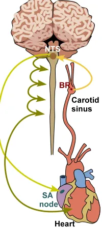
As shown in Figure 1, a change in upper body blood pressure imposed by postural change such as head-up

tilt (HUT) stimulates firing of afferent stretch sensitive baroreceptor neurons terminating in the aortic arch

and carotid sinuses. The signals generated by the afferent neurons are integrated in the Nucleus of the

Solitary Tract (NTS) from which it is transmitted within the brain stem to the sympathetic and

parasympathetic systems modulating the concentration of neurotransmitters acetylcholine and

noradrenaline at the end organs. Acetylcholine, associated with parasympathetic signaling, has an

immediate effect on heart rate and cardiac contractility, whereas noradrenaline, associated with the

sympathetic system has a delayed (5-7 seconds from the blood pressure stimulation) effect regulating heart

rate, cardiac contractility, and vascular tone [1, 2].

Heart rate regulation and many other biological phenomena, can be modeled mathematically using a

system of coupled nonlinear differential equations with states representing dependent biological variables

and an associated set of parameters representing constant quantities. Typically, parameters representing

physiological quantities, sometimes referred to as biomarkers, can be used to examine differences among

study cohorts. For example, parameters representing timescales or the magnitude of a given response may

be modulated by disease, and can thus serve as biomarkers that can be compared within and between

groups of subjects.

Physiological models are often derived from a mixture of first principles and empirical knowledge. Some

parameters may be measurable, but many may be assigned based on average behavior, in vitro

experiments, literature estimates, or may not be known at all. As a result, models may predict accurate

behavior for an average healthy subject, while it may be difficult to theoretically determine parameters

limited quantities can be measured for practical or ethical reasons and where biological systems can never

be fully isolated. One way to estimate patient specific parameters is via the solution to the associated

inverse problem, which given the system of equations and associated experimental observations provide

estimates of model parameters and initial conditions by minimizing the least squares error between the

model output and observed experimental data.

Typically, inverse problems do not have a unique solution, in particular since data may only be available

for one or a few of the model states, even for problems where the structure allows for identification of

parameters [3–6]. However, it may be possible to uniquely estimate a subset of model parameters by fixing

insensitive and correlated parameters at their nominal parameter values. Parameters are denoted

insensitive if the change in the model output is insensitive to changes in parameters and correlated if two

or more parameters change the model output in the same or complementary manner [4, 7]. Neither

insensitive nor correlated parameters are practically identifiable [3–5, 7]. Many methods for subset

selection [4, 7] are based on sensitivity analysis, which can be either local [8] or global [9]. Local sensitivity

analysis predicts how the model output is changed for given parameter values, while global sensitivity

analysis predicts how the model output is changed as parameters changes within the parameter space

defined by the problem formulation. Local sensitivity analysis is commonly used on steady-state and

time-dependent models and can only account for small variations from the nominal parameter values. On

the other hand, since global sensitivity methods examine effects on the whole parameter space, they are

more applicable for highly nonlinear problems.

One common method for predicting global sensitivities is based on global sensitivity indices (often referred

to as Sobol indices) [10, 11], which predict and decompose the model output variance and attributes this

variance to the parameters and their interactions. The advantage of this and other variance based methods

is that they allow exploration of input space, identifies interactions between input variables and are not

limited to linear responses. The disadvantage is the large computational cost. Other global methods are

the Derivative based Global Sensitivity Measures (DGSM) [8, 12] and Morris Method [13], both

computationally more efficient than Sobol Indices. DGSM is obtained by averaging local sensitivities

predicted for representative parameter sets within the parameter space, while Morris Method is a

one-at-time (OAT) method, that systematically varies parameters one at the time to obtain a measure of

capture effects of input variable interactions [8, 12, 13].

Early uses of sensitivity analysis includes economical and chemical reaction models, but more recently

sensitivity analysis has been applied to biological models. One of the challenges within biological studies is

that observed quantities often are limited compared to the number of model states. While most studies use

local sensitivity methods, some have explored both local and global methods. Examples include studies by

Tur´anyi [14] et al., who analyzed a wide range of chemical reactions associated with pyrolysis, combustions

and stratospheric compounds, and Hamby [15] who provides a short review of local and global sensitivity

analysis methods often used for model design, experiment planning and effects of varying model parameters

in environmental studies. In this study we show that ideas from DGSM method proposed by Kucherenko

et al. [12] can be used to obtain a measure of global sensitivities for the heart rate dynamics model.

The manuscript is organized as follows. First we present a physiological description of the baroreceptor

reflex system and the experimental data used for model validation. Next, the mathematical model is

presented, followed by a derivation of local and global sensitivities. Moreover, we present results of the

sensitivity analysis, ranking model parameters from the most to the least sensitive, and finally, we

demonstrate that sensitivities can be used to estimate bounds for model parameters. In the discussion, we

outline what insights sensitivities have provided that can be used in future studies addressing questions of

parameter identifiability.

Methods

The Baroreceptor feedback control and experimental data

The baroreceptor reflex operates via negative feedback control regulating heart rate, cardiac contractility,

and vascular tone in response to changes in blood pressure [2] (see Figure 1). This control system is often

studied using orthostatic stress tests, where the subject is exposed to procedures involving head-up tilt,

active standing, and lower-body negative pressure. For all tests, the applied task leads to gravitational

pooling of approximately 500 ml blood in the legs, reducing cardiac filling and thus blood pressure, which

in turn stimulates heart rate, cardiac contractility, and vascular tone.

Baroreceptors are stretch sensitive nerve fibers located at the carotid sinus and the aortic arch that senses

changes in arterial blood pressure [2]. A drop in blood pressure leads to a decrease in the firing rate of the

pathways are activated via the autonomic nervous system: The sympathetic and the parasympathetic

systems. Upon HUT, blood pressure in the upper body drops inhibiting firing of the baroreceptor nerves.

In turn, the parasympathetic system is inhibited, while the sympathetic system is stimulated.

Parasympathetic outflow is mediated by the vagus nerve, which mainly consists of large myelinated nerve

fibers with fast conduction and operates via modulation of the neurotransmitter acetylcholine.

Sympathetic activation is mediated through small unmyelinated nerve fibers with slow conduction and

triggers the release of noradrenaline via a network of slow conducting neurons. Due to slow conduction the

modulation of heart rate by the sympathetic system occurs with a delay of about 5-7 seconds whereas the

modulation caused by the fast conducting parasympathetic system occurs within a second.

In the heart, pacemaker cells initiate the electrical impulses causing contraction. Acetylcholine and

noradrenaline affects the rate of transportation of ions through the cell membrane and the level of

electrical potential required for contraction [2]. During head-up tilt the concentration of acetylcholine

decreases, inhibiting the damping of heart rate, whereas an increase in noradrenaline stimulates heart rate.

The baroreceptor reflex is often compromised in patients suffering from orthostatic intolerance [16, 17].

This syndrome is typically diagnosed using tilt-table tests monitoring changes in blood pressure and heart

rate, the only signals that can easily be measured noninvasively in the clinic. These data represent input

and output within a complex chain.

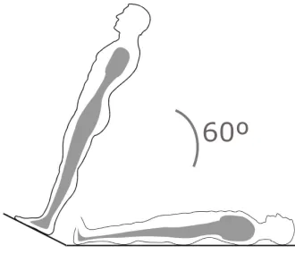
During the test, the subject is initially resting in supine position, until steady levels for blood pressure and

heart rate have been recorded. At this stage the table is tilted to 60◦

which triggers the baroreceptor

reflex. Figure 2 illustrates the experimental setup and Figure 3 shows a set of measured data. During the

experiment, heart rate is measured using a standard 3-lead ECG (FE135 Dual Bio Amp, AD Instruments

Inc, Colorado Springs, CO, USA), while blood pressure is measured using finger photoplethysmography

(Finometer, Finapres Medical Systems B.V., The Netherlands). For the data analysis presented in this

paper we extracted data from a 10 minute interval around the tilt. Data were sampled at 1 kHz, but

subsampled to 50 Hz for computational analysis. The experimental setup was approved by the internal

review board at Frederiksberg Hospital, Denmark and the subjects included in the study provided written

Baroreflex modeling

Numerous modeling studies have addressed baroreflex regulation (e.g. [18–20]), however, most of these only

analyzed some aspects of the system, and most were validated against literature and animal data. To our

knowledge, only a few models have described the complete system from blood pressure to heart rate

regulation [21, 22]. One of the obstacles in designing patient specific models is that human data are only

available at the ends of the chain: blood pressure, which serves as an input to the system and heart rate,

the model output.

The mathematical model investigated in this study incorporates the parts of the negative baroreflex

feedback system that modulate heart rate. It is described by coupled differential equations predicting

blood pressure changes, afferent baroreceptor firing rate, sympathetic and parasympathetic outflow,

concentrations of the neurotransmitters acetylcholine and noradrenaline, and the change in electrical

potential of the pacemaker cells, from which heart rate is predicted (see Figure 4). The model is motivated

by previous studies [7, 21–24], but is modified in a number of ways: First, equations describing afferent

firing are nondimensionalized eliminating a parameter from the system, a distributed delay is incorporated

instead of a fixed delay, and heart rate potential is modeled accounting for electrical stimulation of the

pacemaker cells. In the following, each component of the model is outlined.

Baroreceptor firing

The activity of the afferent baroreceptor neurons of typei(ni) are modulated in response to changes in

blood pressure. It is known that several neuron types exist, and that they can be separated according to

their ability to conduct the signal. Similar to previous studies [21, 23] we assumed, that three neuron types

can be differentiated, and that the activity of each neuron can be predicted by

dni

dt =ki

dpm(t)

dt

n(M−n) (M/2)2 −

ni−Ni

τi

, n=Xni, N =

X

Ni, (1)

whereNi is the threshold firing rate for each neuron type, N is the total firing rate threshold,nis the

current total firing rate,M is the maximum firing rate,ki is a constant determining how sensitive the

receptor is to changes in blood pressure,τi is a time constant that determines the rate at which the firing

rate decays to the threshold value, and dpm/dtis the rate of change of the mean blood pressure given by

dpm

wherep(t) is a linear interpolation of the experimental pressure data. The solution to (2) smooths the input pressure, providing a weighted average given by

pm(t) =

Z t

−∞

e−a(t−s)_{p(s) ds, (3)}

wherea= 1.5 is a parameter that describes the shape of the profile used for the weighted average.

The parasympathetic outflowTp and the parasympathetic thresholdTp0 are defined as

Tp=

n

M, Tp0= N

M. (4)

Introducing the nondimensionalized quantitiesνi= (ni−Ni)/M with derivatives, the two equations above

can be rewritten as

dνi

dt =κi

dps

dt Tp(1−Tp)− νi

τi

, κi=

4kipmax

M , Tp= X

i

νi+Tp0, (5)

where the pressurepsis obtained by scaling the input pressurep(t) bypmax= 200 mmHg, i.e.

dps

dt =a _p(t)

pmax −

ps

. (6)

In the above equations, the firing rate must be positive and smaller than the maximum firing rate, i.e.

0< N≤M, consequently, 0< Tp0≤1.

As described earlier the sympathetic signal is mediated to the heart via a complex network of neurons,

which in previous studies [21, 22] were accounted for by introducing a fixed time delay. However, delay

equations are difficult to solve numerically [25], which make sensitivity analysis nontrivial [26] and in

addition discrete/sharp time delays hardly appears in biological neuronal networks. To avoid the added

complexity, we follow ideas from [27, 28] for implementing distributed delays by defining the delayed

parasympathetic outflow as

Tp,d=

Z t

−∞

Tp(η)gρα(t−η) dη, gαρ(u) =

αρ_uρ−1_e−αu

(ρ−1)! , (7)

whereαandρare integers that determines the shape of the gamma distribution used as weight for the signal. Weighting functions with a mean delaytd =ρ/α= 6 for different values ofρare shown in Figure 5.

It is worth noting that the limiting case whereρ→ ∞results in the Dirac delta function [28]. Expanding and rewriting (7) yields

Tp,d=kTdρ, k=

αρ

(ρ−1)!, T

ρ d =

Z t

−∞

Differentiation for eachρgives a simple system of differential equations of the form

dT_dρ

dt = (ρ−1)T

ρ−1

d −αT ρ d,

.. .

dT1

d

dt =Tp(t)−αT

1

d.

(9)

For this studyρ= 5 representing a trade-off between a narrow distribution and fewer differential equations. A physical interpretation of these equations would be that the delay is generated as the signal is passed

through a series of compartments.

Using the distributed delay, the sympathetic outflow is predicted as

Ts=

1−Tp,d

1 +βTp

, (10)

whereβ is a constant controlling the damping of the sympathetic Tsoutflow by parasympatheticTp.

The normalized concentration of the neurotransmitters acetylcholineCa and noradrenalineCn are

predicted from first order kinetics

dCa

dt =

Tp−Ca

τa

, dCn

dt =

Ts−Cn

τn

, (11)

whereτa andτn are time constants.

Finally, the build-up of electrical potentialφin the pacemaker cells is determined by

dφ

dt =H0−MaCa+MnCn, (12)

whereH0denotes the default depolarization rate when no neurotransmitters impact the system, and

Ma, Mn denote the sensitivity to the normalized neurotransmitter concentrations. This model reflects only

the pre-potential of the pacemaker action potential, and ignores effects on Ca++, Na+ and K+ gates in the

remaining period of the cycle.

In earlier studies of this model [7, 22] an increase in electrical potential of 1 would determine the time

between the most recent contraction atta and the next attb,

1 =

Z tb

ta

φ(t) dt. (13)

Between these time points the heart rate is the inverse of the difference of the times, 1/(tb−ta). However,

when comparing the model output to experimentally measured values due to the discrete nature of these

data. Notice that the time points for model and experimental data do not coincide. While interpolation

between contractions for model output is a way of handling this discrepancy, we propose another approach.

The discrete format of the heart rate data means that we can only infer information on the average

behavior of the electrical potential between contractions. Hence, we will calculate the heart rate between

two time pointsta andtb as the average increase in the potential over this period,

H(tb) =

φ(tb)−φ(ta)

tb−ta

, (14)

where an increase in electrical potential of one corresponds to a contraction. For the model to behave as

intended all parameters values must be greater than 0 and the parameter 0≤Tp0≤1.

Model summary The mathematical model described above can be summarized as follows

dx

dt =f(x, p(t), t;θ), x(0) =x0, θ=

H0, Mn, Ma, τa, τn, β, κ1, κ2, κ3, τ1, τ2, τ3, td, Tp0 , (15)

x=

φ, Ca, Cn, ν1, ν2, ν3,p, T¯ d5, Td4, Td3, Td2, Td1 ,

wherexdenotes the 12-dimensional state variable,p(t) the input function,t the independent variable, and

θthe 14-dimensional parameter vector. In this study, we have adopted values from [22] whenever possible, see Table 2.

The model output, heart rate is a function of the state variables and time,

H(tn) =g(tn, tn−1, x(tn), x(tn−1)). (16)

wheretn denotes then’th point in time where output is sampled. Note that for our specificH the

dependence on the state variable is only onφ(t).

Sensitivity analysis

Sensitivity analysis investigates the influence that changes in parameter values have on the model output.

For studies where data are available, sensitivities are evaluated at time-points where data are recorded.

Classically [29, 30], sensitivities are local, i.e. they are evaluated at given parameter values. However, for

models for which the output is nonlinear in the parameters, local sensitivities do not accurately predict the

sensitivities should be computed. In this study, we predict both local and global sensitivities and discuss

their impact on heart rate.

Local sensitivities

The local sensitivity matrix for model outputsy to the parametersθ is defined as the derivative

S=∂y/∂θ. For the studies presented here we assume that the model outputy=g(x, t;θ) is a function of the model states, time and parameters, i.e.

S= ∂ y

∂θ = ∂ g ∂x

∂ x ∂θ +

∂ g ∂θ

depend on the local sensitivities for each of the statesSx=∂x/∂θ. Denoting the number of model states

Nxand the number of parametersNθ, we obtainNx×Nθ differential equations, whose solution contain the

local sensitivities for each state. For a model described by (15) sensitivities can be computed as solutions to

d dt

∂x ∂θ

= ∂f(t, x, θ)

∂θ +

∂f(t, x, θ)

∂x ∂x ∂θ

d

dt (Sx) = Jθ+JxSx, (17)

whereJθ=∂f(t, x, θ)/∂θ andJx=∂f(t, x, θ)/∂xare the parameter and model Jacobian.

Sensitivities can be predicted by deriving all sensitivity equations explicitly [31], however, for large systems

with many parameters this approach is not feasible. Alternatively, one can use automatic differentiation,

which uses semi-analytical methods for the calculations of the model and parameter Jacobian [32]. In

Matlab, these methods are difficult since they typically rely on parameter overloading [33]. Finally, one

could use some version of finite differences directly predicting sensitivities [34]. For this study, we predicted

sensitivities using finite differences, but took advantage of the numerical solver CVODES [35] to solve (17).

The equations associated with prediction of heart rate dynamics are fairly stiff, consequently they were

solved using BDF and Newtons method. An advantage of Newtons method is that it involves calculation of

the model Jacobian, therefore the additional expense involved with predicting sensitivities is negligible.

The only additional cost is due to calculating the parameter Jacobian which is approximated by finite

differences by CVODES.

The model output, heart rate, is a discrete quantity and as such prediction of sensitivities of model output

function of the statesx, as described by (16)

sy_j(tn) =

∂y(tn)

∂θj

= ∂g(tntn−1, x(tn), x(tn−1))

∂θj

= ∂g(tn, tn−1, x(tn), x(tn−1))

∂x(tn)

∂x(tn)

∂θj

+∂g(tn, tn−1, x(tn), x(tn−1))

∂x(tn−1)

∂x(tn−1)

∂θj

.

For the model introduced, equation (14) takes on the role of the functiongand only involves one state. So for our model,

y(tn) =g(tn, tn−1, x(tn), x(tn−1)) =

x(tn)−x(tn−1)

tn−tn−1

. (18)

Hence, the sensitivities can be found as

sy_j(tn) =

∂y(tn)

∂θj

= ∂g(tntn−1, x(tn), x(tn−1))

∂θj

=

∂x(tn)

∂θj −

∂x(tn−1)

∂θj

tn−tn−1

= sj(tn)−sj(tn−1)

tn−tn−1

, (19)

wheresj is the sensitivity of the state variable thatg depends on to thej’th parameter.

For many models, including the one analyzed here, model parameters vary by several orders of magnitude.

For example, as noted in Table 1, parameters associated with the baroreflex model vary four orders of

magnitude. To ensure prediction of relative sensitivities, the parameters and model output are scaled

logarithmically. Thus, we define ˆθ= ln(θ) and ˆy= ln(y) and predict sensitivities ass=∂y/∂ˆ θˆ, giving

Sj(tn) =

∂logy(tn)

∂logθj

= ∂y(tn)

∂θj

θj

y(tn)

=sy_j(tn)

θj

y(tn)

, y(tn)6= 0. (20)

To calculate the local relative sensitivities for the model, (18), (19) and (20) are combined to form the

expression

Sj(tn) =

sj(tn)−sj(tn−1)

x(tn)−x(tn−1)

θj. (21)

Global sensitivities

The model studied here is nonlinear both in the states and in the parameters. This is important as the

model sensitivities are functions of model parameters and therefore change nonlinearly for different

parameter values [4, 8]. Thus, local sensitivities predicted from nominal parameter values do not accurately

reflect parameter sensitivities over the full parameter space. To assess the reliability of local sensitivities

for the baroreceptor reflex model, this study compares local and global sensitivities.

To limit computational overhead, we use an approach inspired by Kucherenko et al. [12] and Kiparisides et

sensitivities over the relevant parameter intervals, and by combining it with a measure of the variance in

the sensitivities creates an overall ranking of the parameters.

Global sensitivitiesSglobal are approximated as the average of local sensitivitiesS over the parameter space

defined byP. More specifically, global sensitivities are obtained by integrating the local sensitivities and

dividing by the volume covered, i.e.

S_{global =} R

PS(t, θ) dθ

R

Pdθ

, (22)

whereθ denotes the parameter vector. It should be noted that if sensitivities to a given parameter changes from positive to negative the global sensitivities of this parameter may be underestimated.

The integral is approximated by a sum of sensitivities overN points in the parameter space

ˆ

S_{global =} 1 N

N

X

i=1

S(t, θi), (23)

whereθi∈ P, i= 1, . . . , N.

Different methods exist for choosing the points in the parameter spaceθi. The simplest approach uses

Monte Carlo integration, which picks theN points randomly [36]. The disadvantage of this method is the high number of evaluations required to get a good approximation of the integral. Another possibility is

calculating the global sensitivities using sparse grid integration [37–39], which generalizes Gaussian

quadrature rules to higher dimensions, though this method is significantly more complex to implement. A

popular method balancing computational cost and feasibility utilizes Sobol sequences [40, 41] for selection

of evaluation points. As the nameSobol sequences might cause a wrong associations to Sobol Indices, in

the remainder of this study these will be denotedlow-discrepancy sequences. This method is often referred

to as quasi-random Monte Carlo integration and has the advantage, that the distribution of points in the

space is more uniform. This is illustrated in Figure 7, where the points selected for a two dimensional

space is shown, for a quasi-random sequence and for random numbers generated by regular Monte Carlo

integration. The more uniform distribution results in faster convergence, with the error being proportional

to ln(N)/N for quasi-random integration compared to 1/√N for regular Monte Carlo integration [36]. For this study, we used the quasi-random (Sobol) sequence implementation available within the GSL

libraries [42].

In summary, to obtain the global sensitivitiesN parameter sets are selected using sequences,

Results

We have calculated local and global sensitivities for the nonlinear heart rate model. Sensitivities were

compared over the parameter space given in Table 1. Below we first show examples of local and global

sensitivities for representative parameter values. These results were analyzed further and used for

bounding the parameter space. Finally, we ranked local and global sensitivities and discuss the impact on

heart rate dynamics. The latter will be done both from mathematical and physiological principles.

Local sensitivities

Local sensitivities depend on the parameter values for which they were computed. For models where

nominal parameters can be predicted, and where nonlinearities have a minor effect, results from local

analysis may be adequate for analyzing the model behavior. However, for models where limited

information is available for estimation of nominal parameters or where the model is known to be very

nonlinear, local sensitivities can be misleading.

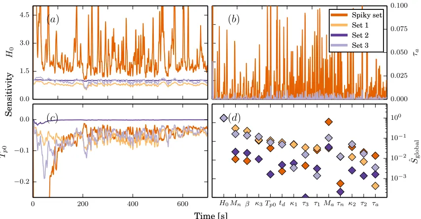
Figure 8 shows local sensitivities for a parameter set causing spiky behavior as well as for three additional

parameter sets. One parameter set represent the nominal parameter values, and two sets were selected at

random from the parameter space listed in Table 1. Graphs include representative time-traces for

parametersθ={H0, τa, Tp0}. The three panels were chosen to show behavior for parameters within the

allowed parameter space. Recall, that all parameters are assumed positive.

Finally, the panel in the bottom right corner shows the two norms for each parameter set,

||Sˆ||2=

M

X

i=0

S(ti, θ)2

!

1 2

.

Both time-varying sensitivities and relative ranking depend on the sampling values, and, for some

parameter sets, on sensitivity spikes. The maximum values for the spiky sensitivities is significantly larger

than depicted in Figure 8, but the y-axis was cropped to show all traces. Note that,

1. The sensitivities forH0is very similar in magnitude for most parameter sets.

2. One parameter sets give rise to very large and rapid fluctuations in the sensitivities. For the

3. Ranking of the most sensitive parameters remain the same for all parameter sets, while the ranking

of the less sensitive parameters vary among the four sets.

From these observations it is clear that the effect may differ for different parameters and for different

points in the parameter space. This imply that the relationship between parameters change depending on

the parameter values. Finally, we noted thatspiky sensitivities may contribute excessively when calculating

global sensitivities.

Spiky sensitivities

Figure 8 shows that there exist parameter sets for which the time-varying sensitivities spike at certain

values in time. First, recall that sensitivities are relative, i.e. for a given value in time the sensitivitySi(tj)

can be large or approach infinity if the absolute sensitivitysi(tj) is large, if the parameterθi→ ∞, or if

the model output (heart rate)y(tj)→0. Since all parameters are bounded, a spike can only appear if the

absolute sensitivitysi(tj)→ ∞or if the model outputy(tj)→0.

To better understand what combinations of parameters that gave rise to spiky sensitivities, we saved all

parameter sets resulting in relative sensitivities larger than 5. Local sensitivities were predicted at 50,000

points sampled by low-discrepancy sequences and of these 446 were marked as spiky. Figure 11 shows

histograms for the 446 spiky parameter sets. For each panel thex-axis give the parameter bounds. First note that parametersH0, Tp0, Ma, andMs do not follow the uniform distribution expected for

low-discrepancy sequences. In particular, it should be noted that small values ofH0 andTp0→1 gives rise

to spiky sensitivities.

To investigate the relation betweenH0 andTp0further, Figure 12 shows a two-dimensional histogram of

the pair-wise distribution (similar graphs could be generated for all parameters with a nonuniform

distribution). The scale goes from no occurrences of the parameter combination, represented by the blue

color, to many combinations represented by red. This figure shows thatTp0→1 gives rise to a spiky

sensitivity independent of the value ofH0. Moreover, it shows that spiky behavior can be generated for

other values ofTp0 ifH0 is sufficiently small. On a molecular level parasympathetic stimulation, as caused

by large baroreceptor firing, closes the f-channels available for ion current through the membrane of the

pacemaker cells, inhibiting potential build-up and decreasing heart rate. Since sympathetic stimulation of

stimulation will be inhibited at increased parasympathetic activity.

This relation betweenH0 andTp0 is not immediately obvious from the model equations. H0determines the

baseline heart rate with no nervous system stimulation andTp0 determines the baseline firing rate of the

baroreceptors as shown in (5) and (12). Earlier we noted the possibility of large values in relative

sensitivity to be caused by low values of heart rate. It is clear that small values ofH0 would lead to a low

heart rate. On the other hand, Figure 12 suggests thatTp0→1 plays an even larger role in causing spiky

behavior. Looking back at (5) and following the effects through the model, we see that a large value ofTp0

leads to large stimulation from the baroreceptors, which means that the sympathetic activity (10) is

lowered significantly while the parasympathetic activity (5) is increased. This cause an increased

acetylcholine concentration and a decreased noradrenaline concentration (11), which in turn causes a very

low, or even negative, change in electrical potential (12). A very low increase in potential (12) will result in

low values of heart rate, which cause spiky behavior. This corresponds to the physiological effect where

strong parasympathetic stimulation of the pacemaker cell affects acetylcholine dependent potassium

channels, decrease the resting potential of the cell and cause zero heart rate. However, negative values of

the potential (12) corresponds to the pacemaker losing potential, which could be interpreted as negative

heart rate.

Faulty parameter sets

In addition to recording the spiky parameter sets, we recorded parameter sets that resulted in a negative

heart rate or made the ODE solver fail. Of 50,000 samples, this behavior was noted 8,256 times.

Histograms showing the distribution of parameter values for these parameter sets are shown in Figure 11.

We denote an error associated with prediction of negative heart rates amodel error, while an error

associated with a parameter set causing the ODE solver to fail is denoted asolver error. The histograms in

Figure 11 reveal that parametersH0 andTp0 also cause model or solver errors. This is likely due to the

prediction of very small or negative values of heart rate.

Other situations in which parameters give rise to nonuniform distributions are when time constants

τa, τ1, τn, andτd reach their lower bound. The parameterτa was bounded by 0 and appears in equation

(11) predicting acetylcholine concentration. Whenτa→0, the value of ddCta → ∞, which cause fast

fluctuations in acetylcholine concentration and in turn make the ODE too stiff for the ODE solver.

larger, and near-zero values are less frequent. The parametertd is used to describe the distributed delay

through the equationα=ρ/tdand plays a role similar to the other time constants. In summary, low values

for time constants give rise to a rapidly changing system, leading to ODEs that become increasingly stiffer,

eventually causing the numerical ODE solver to break. To remedy this problem, the lower bound for these

small time-scales should be set significantly above zero. New bounds are suggested in Table 1. However,

finding an exact lower bound based on biological considerations may be difficult, thus one can anticipate

some parameter sets giving rise to solver errors.

Global sensitivities

Global sensitivities were computed with revised parameter bounds. To obtain accurate predictions local

sensitivities showing spiky behavior or giving rise to either a model or solver error was not included. In

comparison with original bounds, where 8,256 out of 50,000 sets failed, with the revised parameter bounds

only 3,792 out of 50,000 failed, a significant improvement. Figure 11 shows that distributions of parameters

for revised bounds are nearly flat for all parameters.

Even when using low-discrepancy sequences for integration, prediction of global sensitivities is

computationally intensive. Thus, an important question is how many sample values are needed for accurate

prediction. The number depends on the degree of nonlinearity of the model with respect to the parameters,

the number of parameters, and the bounds. To facilitate a discussion on the required number of points

Figure 13 shows global sensitivities calculated using 100, 250, 500, 1,000, 25,000, 50,000 and 150,000

sampling points.

Results show little variation among the most sensitive parameters, while some mid-range and insensitive

parameters varies. Special attention should be given to having enough sampling points to ensure

convergence for the mid-range sensitive parameters, since these may either be included or excluded in

further model analysis.

Results showed that the most sensitive parameters for prediction of heart rate were

Discussion

This study showed that global sensitivity analysis improved prediction of sensitivities for the heart rate

model analyzed in this study. This model is nonlinear, therefore results from local sensitivities are limited

to a small region around nominal parameter values. We showed that the global analysis could be used to

restrict the parameter bounds further beyond values immediately suggested by the biological analysis. We

showed how the discrete time delay used in previous studies [21] can be replaced by a distributed delay

using the linear chain trick and introducing a handful new model compartments. Moreover, this study

included an improved sub-model for prediction of heart rate, obtained by implementing a method for

calculating the average heart rate between two time points.

Necessity of global estimates of sensitivities

To investigate the necessity of global sensitivity estimates we calculated relative sensitivities for the

baroreceptor model. We did this for four different parameter sets (values of parameters are given in Table

2). Figure 8 panel D shows the two-norm of these sensitivities for the different configurations. The

parameters are ordered from the most to the least sensitive based on the sensitivities calculated for the

nominal parameter values, and all are relative to the highest two-norm measured for this configuration. All

of the configurations have a similar sensitivity to the default heart rateH0, while sensitivities to other

parameters vary prominently. These results indicate that it is relevant to seek a global estimate of

sensitivities.

When predicting global sensitivities we found that some parameter sets induced spiky behavior (very large

spikes in the relative local sensitivities) or caused model errors (negative heart rate) or solver errors (solver

failing to converge). These sets were recorded and analyzed further.

Spiky behavior, model and solver errors

We found that the characteristics of parameter sets causing spiky behavior could also be recognized in the

parameter sets that caused model or solver errors. Specifically, we found that certain values of the

pacemaker cell threshold depolarization rate,H0, the pacemaker cell sensitivity to acetylcholine,Ma, and

the baroreceptor threshold firing rate,Tp0all have higher frequency of spiky behavior and model errors.

This behavior was hinted by the nonuniform distributions for these parameters in Figure 11, and

behavior is caused by near zero model output heart rate due to computation of relative sensitivities

whereas negative heart rate will cause model errors. We consider spiky behavior to be the limiting

behavior observed before parameters reach values where they cause model errors.

In addition to revealing the roles of these parameters, Figure 11 panel (b) also showed nonuniform

distributions for most time-scale parameters. Our analysis showed that the values overrepresented in the

histogram for these parameters are the values causing rapid fluctuations, and thus leading to stiff behavior

in the model. Differential equations showing this behavior is referred to as being stiff, which means that

the numerical solver is not able to integrate the equations using step sizes possible with the computer.

Based on these findings we adjusted the intervals for the integration for the timescale parameters causing

stiff behavior and solver errors. The unadjusted and adjusted parameter intervals are listed in Table 1.

Figure 11 shows that after this adjustment the primary contributor to errors is combinations of large

values ofTp0 and small values ofH0. In addition the number of parameter sets leading to errors is reduced

from 8,256 down to 3,516.

Converge to global estimates

To determine how many points are required in the calculation of global sensitivities we calculated global

sensitivities using nominal parameter values and 100, 250, 500, 1,000, 5,000, 10,000, 25,000, 50,000 and

150,000 different points in the parameter space. Figure 13 shows the results obtained both when including

and excluding spiky sensitivities. We see that the sensitivities calculated using nominal parameter values

do not correspond to the global estimates. The sensitivities to each parameter is different and so is the

order. We also see that for the global estimates there is very little difference between using 100 points and

150,000 points. Looking at the baroreceptor time constantτ3 we see that we can distinguish the result

obtained using 100 points and the nominal parameter set from the rest. This deviation seems to be the

same whether spiky sensitivities are included or not. We see that sensitivities converge as the number of

points is increased. In addition it should be noted that the sensitivities obtained using nominal parameter

values and those obtained by integration show very similar qualitative behavior.

Looking at Figure 13 again we focus on the parameter describing the baroreceptor firing rate thresholdTp0.

There is a notable difference between the graphs produced when including and excluding spiky sensitivities.

time varying sensitivity toTp0shows very similar qualitative behavior for the different time series, and it

appears that increasing the number points in the integration leads to the integral converging to some time

series. However, forTp0 we see a very clear difference in the global estimates obtained when using 1,000

points between the two graphs. When including spiky behavior sensitivities we obtain a very large increase

in the (absolute) sensitivity. This is caused by one of the points included in the low-discrepancy sequence

when going from 500 to 1,000 points. Also note that this only happens forTp0and not for τ3. This would

indicate that either the spiky behavior in this particular case is not due to low model output heart rate as

expected, or that the sensitivity toτ3for this particular configuration is extraordinarily low.

From the investigation of the convergence of the integral for global sensitivities we learn that, the

sensitivity estimate convergence if more points are included, that some parameter sensitivities will be

distorted when including spiky sensitivities and some will not. In conclusion it is important to select good

parameter intervals to avoid spiky sensitivities, as this might greatly reduce the computational effort

required to estimate global sensitivities.

Conclusions

We implemented a heart rate predicting baroreceptor reflex model. We scaled the baroreceptor model

reducing the number of parameters, implemented the sympathetic outflow delay as a distributed delay and

calculated heart rate in a manner that allows for easy comparison to data.

We calculated global sensitivities by averaging local sensitivities based on partial derivatives, giving a

computational advantage when compared to Sobol indices [11] and adding more information than local

sensitivities. The integration used in the averaging was done using a quasi-Monte Carlo method using

low-discrepancy (Sobol) sequences [40].

In addition to calculating global sensitivities we analyzed parameter sets causing negative heart rates,

ODE solver failure or unwanted rapid fluctuations in sensitivities. We call this fluctuating behaviorspiky

behavior and it is caused by low model output. Our analysis gives insight into model dynamics,

relationship between parameters and permit better choice of parameter intervals for integration.

Competing interests

Authors contributions

All authors contributed to preparation of the manuscript, Olsen carried out all computations and analysis,

Tran and Olufsen contributed to formulation of methodologies used for local and global sensitivity analysis,

and Ottesen and Olufsen participated in model formulation and to analysis of sensitivity results on the

heart rate model. Mehlsen was responsible for the integrity of description of pathways associated with

baroreflex regulation and he contributed to the analysis of model results. All authors contributed to

writing the manuscript.

Acknowledgements

Olufsen, Tran, Olsen, and Ottesen were supported in part by National Science foundation under award

NSF/DMS1022688, Olsen was supported by Carl and Katy Kajsings foundation, Olsen and Olufsen

additionally supported by the VPR project under NIH-NIGMS award #1P50GM09450301A0 sub-award to

NCSU. Tran was additionally supported by NIAID 9R01AI071915, Ottesen was supported by carpenter

Sophus Jacobsen and wife Astrid Jacobsen foundation.

References

1. Ottesen JT:Modelling of the baroreflex-feedback mechanism with time-delay.J Math Biol 1997, 36:41–63.

2. Hall JE:Guyton and Hall textbook of medical physiology. Philadelphia, PA: Saunders/Elsevier 2011.

3. Hengl S, Kreutz C, Timmer J, Maiwald T:Data-based identifiability analysis of non-linear dynamical models.Bioinformatics 2007,23:2612–2618.

4. Miao H, Xia X, Perelson AS, Wu H:On identifiability of nonlinear ode models and applications in viral dynamics.SIAM Rev.2011,53:3–39.

5. Raue A, Kreutz C, Maiwald T, Bachmann J, Schilling M, Klingm¨uller U, Timmer J:Structural and practical identifiability analysis of partially observed dynamical models by exploiting the profile likelihood.Bioinformatics 2009,25:1923–1929.

6. Xia X, Moog C:Identifiability of nonlinear systems with application to HIV/AIDS models.IEEE Trans Autom Control 2003,48:330–336.

7. Olufsen MS, Ottesen JT:A practical approach to parameter estimation applied to model predicting heart rate regulation.J Math Biol 2013,67:39–68.

8. Kiparissides A, Kucherenko S, Matalaris A, Pistikopolous E:Global sensitivity analysis challenges in biological systems modeling.Ind Eng Chem Res 2009,48:7168–7180.

9. Saltelli A, Ratto M, Andres T, Campolongo F, Cariboni J, Gatelli D, Saisana M, Tarantola S:Global sensitivity analysis: the primer. Chichester, England: John Wiley 2008.

10. Sobol IM:Sensitivity estimates for nonlinear mathematical models.Math Modeling Comput Experiment 1993, 1(4):407–414.

11. Sobol I:Global sensitivity indices for nonlinear mathematical models and their Monte Carlo estimates.Math Comput Simulation2001,55:271–280.

13. Morris MD:factorial Sampling Plans for Preliminary Computational Experiments1991,33:161–174.

14. Tur´anyi T:Sensitivity analysis of complex kinetic systems. Tools and applications.J Math Chem 1990,5:203–248.

15. Hamby D:A review of techniques for parameter sensitivity analysis of environmental models. Environ Monit Assess 1994,32:135–154.

16. Goldstein DS, Sewell L, Holmes C, Pechnik S, Diedrich A, Robertson D:Temporary elimination of orthostatic hypotension by norepinephrine infusion.Clin Auton Res 2012,22:303–306.

17. Shibao C, Okamoto L, Biaggioni I:Pharmacotherapy of autonomic failure.Pharmacol Ther 2012, 134:279–286.

18. Bannister R:Multiple system atrophy and pure autonomic failure. InClinical autonomic disorders: evaluation and management. Edited by PA L, Boston: Little, Brown 1993:517–525.

19. Mosqueda-Garcia R, Furlan R, Tank J, Fernandez-Violante R:The elusive pathophysiology of neurally mediated syncope.Circulation 2000,102:2898–2906.

20. van Heusden K, Gisolf J, Stok WJ, Dijkstra S, Karemaker JM:Mathematical modeling of gravitational effects on the circulation: importance of the time course of venous pooling and blood volume changes in the lungs.Am J Physiol 2006,291:H2152–H2165.

21. Olufsen MS, Tran HT, Ottesen JT, Lipsitz L, Novak V:Modeling baroreflex regulation of heart rate during orthostatic stress.Am J Physiol 2006,291:R1355–R1368.

22. Ottesen J, Olufsen MS:Functionality of the baroreceptor nerves in heart rate regulation.Comp Math Prog Biomed 2011,101:208–219.

23. Ottesen JT:Non-linearity of baroreceptor nerves.Surv Math Ind Springer-Verlag 1997,7:187–201.

24. Olufsen M, Tran H, Ottesen JT:Modeling cerebral blood flow control during posture change from sitting to standing.Cardiovasc Eng 2004,4:47–58.

25. Bellen A, Zennaro M:Numerical methods for delay differential equations. Oxford: Oxford University Press 2013.

26. Banks H, Robbins D, Sutton KL:Generalized sensitivity analysis for delay differential equations. In Control and Optimization with PDE Constraints, Basel, CH: Springer 2013:19–44.

27. MacDonald N:Time lags in biological models. Berlin: Springer-Verlag Heidelberg 1978.

28. Smith H:Distributed Delay Equations and the Linear Chain Trick. InAn Introduction to Delay Differential Equations with Applications to the Life Sciences,Volume 57 of Texts in Applied Mathematics, New York: Springer 2011:119–130.

29. Frank PM:Introduction to system sensitivity theory. New York: Academic Press 1978.

30. Eslami M:Theory of sensitivity in dynamic systems: An introduction. Springer-Verlag 1994.

31. Ellwein LM, Tran HT, Zapata C, Novak V, Olufsen MS:Sensitivity analysis and model assessment: Mathematical models for arterial blood flow and blood pressure.Cardiovasc Eng 2008,8:94–108.

32. Griewank A, Walther A:Evaluating derivatives: principles and techniques of algorithmic differentiation. Philahelphia, PA: Siam 2008.

33. Bischof C, Lang B, Vehreschild A:Automatic differentiation for matlab programs.Proc Appl Math Mech 2003,2:50–53.

34. Pope SR:Parameter identification in lumped compartment cardiorespiratory models. ProQuest 2009.

35. Serban R, Hindmarsh A:CVODES, the sensitivity-enabled ODE solver in SUNDIALS.Proc ASME Int Design Eng Techl Conf 2005.

36. Press WH, Teukolsky SA, Vetterling WT, Flannery BP:Numerical recipes in C: The art of scientific computing. New York 1997.

37. Novak E, Ritter K, Schmitt R, Steinbauer A:On an interpolatory method for high dimensional integration.J Comput Appl Math 1999,112:215–228.

39. Bungartz HJ, Griebel M:Sparse grids.Acta numerica 2004,13:147–269.

40. Sobol I:On the distribution of points in a cube and the approximate evaluation of integrals.USSR Comput Math Phys 1967,7:784–802.

41. Joe S, Kuo F:Remark on algortihm 659: Implementing Sobol’s quasirandom sequence generator. ACM Trans Math Software 2003,29:49–54.

Figures

Figure 1

Baroreceptors in the carotid sinus and the aortic arch generates nerve impulses in response to changes in

pressure. The signals are integrated in the NTS and the sympathetic and parasympathetic outflows are

generated. The sympathetic outflow is mediated down the ganglia, an interconnected network of neurons

located in the spine, while the parasympathetic signal is mediated by the vagus nerve. At the heart level

Figure 2

When the subject is tilted from supine position to an angle of 60◦ _{blood is pooled in the lower extremities}

causing increased blood pressure and volume in the lower body, while decreasing the blood volume and

pressure in the upper body. Pressure changes at the carotid sinus will stimulate baroreceptors, thereby

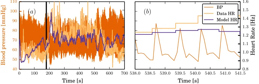
Figure 3

(a) shows experimentally measured blood pressure (BP) and heart rate (Data HR) as well as the heart rate

generated by the model (Model HR) using nominal parameter values. The subject starts the experiment

horizontally and undergoes a HUT to 60◦ _{at t= 180 seconds as indicated by the black vertical line. Note}

the dramatic drop in blood pressure and increase in heart rate immediately following the tilt. (b): Zoom

fort= 300 to 303.5 seconds reveal the short term fluctuations of the blood pressure as well as the discrete nature of the heart rate.

0 100 200 300 400 500 600 700

Time [s] 40 50 60 70 80 90 100 110 B lo o d p re ss u re [m m H g ]

538.0 538.5 539.0 539.5 540.0 540.5 541.0 541.5

Time [s]

0.8 0.9 1.0 1.1 1.2 1.3 1.4 1.5 1.6

H e a rt R a te [H z ] BP Data HR Model HR

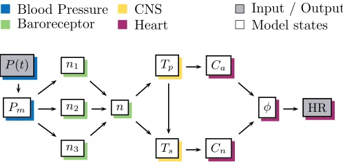
Figure 4

A schematic view of the model components included to predict baroreflex regulation of heart rate during

HUT.P(t) is the blood pressure model input,Pm(t) smoothed relative blood pressure,n1, n2, n3the tone

from baroreceptors with three different inherent timescales,nthe total firing rate of baroreceptors,Tp, Ts

the parasympathetic and sympathetic outflow,Ca, Cn the concentration of acetylcholine and noradrenaline,

φthe cumulative pacemaker potential buildup and HR the model output: heart rate.

rs _{Blood Pressure}

rs _Baroreceptor

rs _CNS rs _Heart

r

s _{Input / Output} rs _{Model states}

P(t) n1 T_p C_a

Pm n2 n φ HR

Figure 5

Shape of the weighting functiongρ

α(u) for different values ofρ, all with same mean delaytd=ρ/α= 5 and

α= 1. The weighting function withρ= 5 is used for the delay of the sympathetic pathway, whileρ= 1 (andα= 1.5) is the one used to smooth the input pressure data in (2) and (3).

u

g

ρ a(

u

)

ρ= 1

ρ= 3

ρ= 5

ρ= 10

ρ= 20

0 0

2 4 6 8 10 12 14

Figure 6

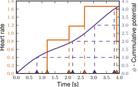
Experimental heart rate (orange) is the inverse of time between the last two heart contractions, 1/(tb−ta).

Time points for contraction in data is illustrated by orange triangles on the time axis. Determining time

between contractions for the model as the time required for potential to increase by one,Rtb

taφ(t) dt= 1, would lead to contractions as illustrated by the purple triangles. Note that data and model times do not

coincide. Instead model heart rate is the average increase inφ(purple) over the same period,

(φ(tb)−φ(ta))/(tb−ta). This ensures that data and model output is available for the same points in time.

0.0 0.5 1.0 1.5 2.0 2.5 3.0 3.5 4.0

Time [s]

0.0 0.2 0.4 0.6 0.8 1.0 1.2 1.4 1.6 1.8

H

e

a

rt

ra

te

0.0

0.5

1.0

1.5

2.0

2.5

3.0

3.5

4.0

4.5

φ

-C

u

m

m

u

la

ti

v

e

p

o

te

n

ti

a

Figure 7

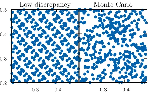
Demonstration of the distribution of points used for numerical integration over a 2-dimensional space using

the quasi-Monte Carlo method with low-discrepancy sequence and using regular Monte Carlo method. The

points generated by the low-discrepancy sequences are more uniformly distributed resulting in faster

convergence for integration.

Low-discrepancy

Monte Carlo

0.3 0.3

0.3

0.4 0.4

0.4

Figure 8

(a-c): Time trace of model sensitivities for parameters{H0, τa, Tp0} for four parameter configurations one

of which causesspiky sensitivities. (d) shows the two-norm with respect to time of sensitivities for all four

parameter sets plotted in the order from most to least sensitive sorted after set 1 (nominal parameter

values).

0.0 0.2 0.4 0.6 0.8 1.0

Time [s] 0.0

0.2 0.4 0.6 0.8 1.0

S

e

n

si

ti

v

it

y

0.0 1.5 3.0 4.5

H0

0.000 0.025 0.050 0.075 0.100

τa

Spiky set Set 1 Set 2 Set 3

0 200 400 600

−0.2 −0.1 0.0

Tp0

H0Mn β κ3Tp0td κ1 τ3 τ1Maτn κ2 τ2 τa

10−3

10−2

10−1

100

ˆ_Sglo

b

a

l

(

a

₎

₍

b

₎

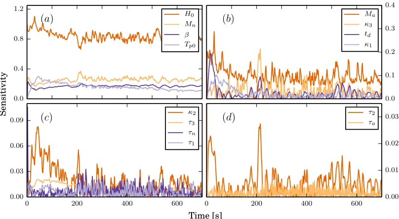
Figure 9

Global sensitivities calculated using 50,000 points in parameter space. The parameters are ordered by their

two-norm from highest in panel (a) to lowest in (d) and the value plotted is the absolute value of the global

sensitivities. Note that the scaling is different in all four sub figures.

0.0 0.2 0.4 0.6 0.8 1.0

Time [s] 0.0

0.2 0.4 0.6 0.8 1.0

S

e

n

si

ti

v

it

y

0.0 0.4 0.8 1.2

H0 Mn β Tp0

0.0 0.1 0.2 0.3 0.4

Ma κ3 td κ1

0 200 400 600

0.00 0.03 0.06 0.09

κ2 τ3 τn τ1

0 200 400 600 0.00

0.01 0.02 0.03

τ2 τa

(

a

₎

₍

b

₎

Figure 10

Sensitivities for a normal and a spiky parameter set. The top row shows the sensitivity to parameterH0,

bottom row the sensitivity to parameterτ1, and middle row shows heart rate for the corresponding model

solution. Left column shows a normal parameter set, middle column a spiky parameter set, and the right

column shows a zoom of the spiky parameter set. Note that the scale on the y-axis is different for the

normal and spiky parameter set, that the heart rate for the spiky solution is near zero and that the right

column shows that spikes in sensitivity coincides with decreases in heart rate.

0.0 0.2 0.4 0.6 0.8 1.0

Time [s] 0.0 0.2 0.4 0.6 0.8 1.0

0.0 0.8 1.6 2.4

S e n si ti v it y -H0 Normal 0 1 2 H R

0 200 400 600

0.00 0.05 0.10 0.15

S e n si ti v it y -τ1 0 4 8 12 Spiky 0 1 2

0 200 400 600 0.0

0.2 0.4

Spiky

Figure 11

(a) Histogram of parameter values that caused local relative sensitivities to exceed five. The figure suggests

that spiky behavior is linked to low values ofH0and large values of Tp0. (b) Histogram of parameter

values that caused the ODE solver to fail. The histograms suggests that low values ofH0 and large values

ofTp0 cause the solver to fail. Likely through the appearance of negative value for ˙φ. In addition time

constants near 0 are over represented. A likely explanation is that small values will cause large and quick

fluctuations, making the equations very stiff. 8,256 parameter sets was found to causes errors.(c) Results when calculating global sensitivities with modified parameter intervals. 3,516 points in parameter space

was found to break the solver - less than half of the number before altering the intervals.

1 2

H0

2 5

Mn

0.1 0.3

Ma

0.2 0.4

τa

0.5 1.0

τn 5 15 β 10 20 κ1 5 15 κ2 15 35 κ3

0.5 1.0

τ1 5 10 τ2 500 1000 τ3 5 15 td

0.3 0.7

Tp0

(a)

1 2

H0

2 5

Mn

0.1 0.3

Ma

0.2 0.4

τa

0.5 1.0

τn 5 15 β 10 20 κ1 5 15 κ2 15 35 κ3

0.5 1.0

τ1 5 10 τ2 500 1000 τ3 5 15 td

0.3 0.7

Tp0

Figure 12

Scatter plot ofH0andTp0 for spiky parameter sets. Values ofTp0near one will induce spiky behavior no

matter the value ofH0. On the other hand ifH0 is largeTp0will also need to be large to induce spiky

behavior, but spiky behavior can also be induced by smaller values ofTp0 ifH0is near zero.

0.00 0.25 0.50 0.75 1.00

H0

0.00

0.25

0.50

0.75

1.00

Tp

0

0 6 12

Figure 13

Top row: Two-norm of global relative sensitivities excluding and including spiky parameters. Middle and

bottom row: Sensitivities to parametersTp0andτ3, excluding (left) and including (right) spiky

parameters. Note the that there is almost no visible difference between the ordering obtained for different

number of points, except for the integration done using 1,000 points. Furthermore the graphs forTp0 and

τ3illustrates that spiky sensitivities might affect the overall output for some parameters. The time series

forTp0also illustrates that spiky parameter that affect the calculated sensitivities.

H0Mn β Tp0Maκ3 κ1 td κ2 τ1 τ3 τ2 τn τa

10−3

10−2

10−1

100

k

ˆ_Sk

2

Excl. spiky par. sets

0 150 300 450 600

−0.4 −0.3

−0.2 −0.1 0.0

ˆ_S

0 150 300 450 600

−0.02 −0.01

0.00 0.01 0.02

ˆ_S

H0Mn β Tp0Maκ3 κ1 td κ2 τ1 τ3 τ2 τn τa

10−3

10−2

10−1

100

Incl. spiky par. sets

0 150 300 450 600

−0.4 −0.3

−0.2 −0.1 0.0 Nominal 100 250 500 1,000 5,000 10,000 25,000 50,000 150,000

0 150 300 450 600

−0.02 −0.01

0.00 0.01 0.02

τ

τ

Figure 14

Global sensitivities calculated using new parameter intervals. They do not appear to be different from the

initial calculated global sensitivities (Figure 9) even though many more points in parameter space was

successfully included in the integration.

0.0 0.2 0.4 0.6 0.8 1.0

Time [s] 0.0

0.2 0.4 0.6 0.8 1.0

S

e

n

si

ti

v

it

y

0.0 0.4 0.8 1.2

H0 Mn β Tp0

0.0 0.1 0.2 0.3 0.4

Ma α κ3 td

0 200 400 600

0.00 0.03 0.06 0.09

κ1 κ2 τ3 τn

0 200 400 600 0.00

0.01 0.02 0.03

τ1 τ2

(

a

₎

₍

b

₎

Tables

Table 1 - Parameter Intervals

Bounds for parameter values used for calculating global sensitivities.

Pre analysis Post analysis

Parameter Minimum Maximum Minimum Maximum

H0 0.00 3.00 0 3.00

Ma 0.00 7.00 0 7.00

Ms 0.00 0.40 0 0.40

τa 0.00 0.60 5×10−2 0.60

τn 0.00 1.50 3×10−2 1.50

β 0.00 20.0 0 20.0

κ1 0.00 30.0 0 30.0.0

κ2 0.00 20.0 0 20.0

κ3 0.00 50.0 0 50.0

τ1 0.00 1.50 7×10−2 1.50

τ2 0.00 15.0 3×10−2 15.0

τ3 0.00 1500 0 1500

td 0.00 20.0 0.3 20.0

Tp0 0.00 1.00 0 1.00

Table 2 - Nominal parameter values

Nominal parameter values used for comparison of local sensitivities for different parameter sets.

Parameter Nominal Set 1 Set 2 Set 3 Set 4 Spiky set

H0 0.94 2.72 1.52 1.47 2.16 0.07

Ma 2.35 6.86 0.60 4.37 0.74 2.80

Ms 0.13 0.18 0.10 0.27 0.26 0.18

τa 0.20 0.11 0.49 0.27 0.32 0.48

τn 0.50 0.41 0.07 0.57 1.18 0.32

β 6.00 8.17 18.6 19.8 14.3 15.6

κ1 10.0 17.9 21.9 1.13 27.1 12.0

κ2 6.67 5.24 9.77 17.7 17.8 13.9

κ3 15.6 30.1 28.9 45.7 16.7 11.3

τ1 0.50 1.09 0.41 1.21 1.07 0.55

τ2 5.00 3.35 6.90 1.51 2.99 10.2

τ3 500 176 1444 393 46.8 855

td 6.00 6.14 11.1 6.91 15.0 10.8