BUSH, BLAKE MARSHALL. Analytical Evaluation of Concrete Penetration Modeling Techniques. (Under the direction of Dr. Emmett Sumner.)
The resistance of concrete targets to penetration of high speed projectiles is a topic of high value in the national security and catastrophic design fields. Many methods have been developed to effectively analyze these types of problems. Currently there are a number of numerical codes and constitutive models used to analyze concrete impact and penetration with new methods developed continuously.
This research evaluates the accuracy of four analysis codes and five concrete constitutive models. Two Lagrangian analysis programs, EPIC and LS-DYNA, as well as an Eulerian code, CTH, are compared in this work. A developmental version of the Material Point
Method is also evaluated in order to study the effectiveness of Arbitrary Lagrangian Eulerian (ALE) modeling methods for concrete impact and penetration. The concrete models
evaluated in this research include Holmquist Johnson Cook, Brittle Failure Kinetics, Osborn, Karagozian and Case, and Drucker-Prager. The modeling programs and constitutive models are evaluated by comparing simulation results to a series of concrete impact and penetration experiments.
by
Blake Marshall Bush
A thesis submitted to the Graduate Faculty of North Carolina State University
in partial fulfillment of the requirements for the Degree of
Master of Science
Civil Engineering
Raleigh, North Carolina
2010
APPROVED BY:
Dr. Murthy Guddati Dr. Sami Rizkalla
LIST OF TABLES ... viii
LIST OF FIGURES ... ix
LIST OF SYMBOLS, ABBREVIATIONS, AND NOMENCLATURE ... xii
1. Introduction ... 1
1.1. Background ... 1
1.2. Objectives ... 2
1.3. Scope ... 3
1.4. Conclusion ... 3
2. Literature Review... 4
2.1. Definition of Concrete Impact... 4
2.2. Modeling Techniques ... 8
2.2.1. Kinematic Descriptions ... 8
2.2.2. Discretization Methods ... 14
2.3. Constitutive Models ... 21
2.3.1. Plasticity Models ... 22
2.3.2. Continuum Damage Models ... 31
2.3.3. Constitutive Models Summary ... 49
2.4. Available Experimental Work ... 49
2.5. Need for Research ... 51
3. Basic Problem ... 53
3.1. Experimental Data ... 54
3.1.1. Projectile ... 55
3.1.2. Target ... 57
3.1.3. Initial and Boundary Conditions ... 60
3.2. Analysis Methods ... 61
3.2.1. Material Models ... 61
3.2.2. Analysis Packages ... 62
3.2.3. Summary of Packages and Models ... 65
3.3. Comparison and Evaluation ... 67
3.3.1. Preliminary Evaluation ... 67
3.3.2. Method Comparison... 67
3.3.3. Experimental Parameter Study ... 68
3.3.4. Evaluation Criteria ... 68
3.3.5. Conclusion ... 71
4. Analytical Investigation ... 73
4.1. EPIC ... 73
4.1.1. Input Data... 74
4.1.2. Material Models ... 75
4.1.3. Contact Definition ... 82
4.2.1. Input Data... 85
4.2.2. Material Models ... 87
4.2.3. Contact Definition ... 92
4.2.4. Output Data ... 92
4.2.5. Code Use ... 93
4.3. CTH ... 94
4.3.1. Input Data... 94
4.3.2. Material Models ... 96
4.3.3. Output Data ... 98
4.3.4. Code Use ... 98
4.4. Material Point Method (MPM) ... 99
4.4.1. Input Data... 99
4.4.2. Material Models ... 100
4.4.3. Output Data ... 102
4.4.4. Code Use ... 103
5. Analysis Pairing Comparison Results ... 108
5.1. Preliminary Evaluation ... 109
5.1.1. Penetration Depth... 110
5.1.2. Projectile Mass Loss ... 111
5.1.3. Deceleration ... 112
5.1.4. Modeling Feature Capabilities ... 120
5.1.5. CPU Run Time ... 121
5.1.6. Conclusions ... 122
5.2. Method Comparison ... 123
5.2.1. Penetration Depth... 124
5.2.2. Projectile Mass Loss ... 125
5.2.3. Deceleration ... 126
5.2.4. Modeling Feature Capabilities ... 136
5.2.5. Run Time ... 136
5.2.6. Conclusions ... 137
6. Experimental Parameter Study ... 139
6.1. Penetration Depth ... 140
6.2. Projectile Mass Loss... 144
6.3. Deceleration ... 148
6.4. Damage Plots... 166
6.5. Conclusions ... 171
7. Conclusions ... 174
7.1. Observations ... 174
7.2. Recommendations for Future Work ... 176
REFERENCES ... 178
1.1. SNL-1 ... 186
1.2. SNL-2 ... 187
1.3. SNL-3 ... 187
1.4. SNL-4 ... 188
1.5. SNL-5 ... 188
1.6. SNL-6 ... 189
1.7. SNL-7 ... 189
1.8. SNL-8 ... 190
1.9. SNL-9 ... 190
1.10. SNL-10 ... 191
1.11. SNL-11 ... 191
1.12. SNL-12 ... 192
1.13. SNL-14 ... 192
1.14. SNL-15 ... 193
1.15. SNL-16 ... 193
2. Experimental Parameter Study Damage Plots ... 194
2.1. SNL-1 ... 194
2.2. SNL-2 ... 195
2.3. SNL-3 ... 196
2.4. SNL-4 ... 197
2.5. SNL-5 ... 198
2.6. SNL-6 ... 199
2.7. SNL-7 ... 200
2.8. SNL-8 ... 201
2.9. SNL-9 ... 202
2.10. SNL-10 ... 203
2.11. SNL-11 ... 204
2.12. SNL-12 ... 205
2.13. SNL-14 ... 206
2.14. SNL-15 ... 207
Table 1. Classification of Impact Response by Velocity (Zukas, 1980) ... 5
Table 2. Classification of Impact Regimes by Impact Pressures and Material Strength (Wilbeck, 1985) ... 6
Table 3. Concrete Impulse Loading Case Studies ... 50
Table 4. Experimental Test Matrix (Forrestal, Frew, Hickerson, & Rohwer, 2002) ... 55
Table 5. Mix Design and Properties of the Experimental Concrete (Forrestal, Frew, Hickerson, & Rohwer, 2002) ... 58
Table 6. Analysis Matrix for Target Material Models ... 66
Table 7. Analysis Matrix for Projectile Material Models ... 66
Table 8. Method Comparison Test Matrix ... 68
Table 9. Sample Grading System... 71
Table 10. JC Material Constants ... 76
Table 11. Osborn Material Constants ... 77
Table 12. HJC Material Constants for Low and Conventional Strength Concretes ... 81
Table 13. Summary of K&C Strength Material Parameters ... 89
Table 14. Summary of K&C Equation of State Material Parameters ... 90
Table 15. Summary of K&C Damage Material Parameters ... 91
Table 16. BFK Material Constants ... 97
Table 17. BFK Reference Equation of State Values ... 97
Table 18. DP Material Constants ... 102
Table 19. Analysis Matrix for Target Material Models ... 108
Table 20. Deceleration Grading for Preliminary Evaluation ... 119
Table 21. Preliminary Evaluation Grading ... 122
Table 22. Deceleration Descending Slope Linear Trend Lines for Method Comparison .... 132
Table 23. Deceleration Grading for the Method Comparison ... 135
Table 24. Method Comparison Run Times ... 137
Figure 1. System Response (Cargile D. , 1998) ... 7
Figure 2. Comparison of Lagrangian, Eulerian, and ALE Descriptions (Donea, Huerta, Ponthot, & Rodriguez-Ferran, 2004) ... 12
Figure 3. Lagrange Interpolation and Shape Functions: a) Linear, b) Quadratic (Cook, Malkus, Plesha, & Witt, 2002)... 16
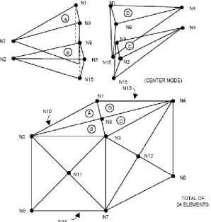
Figure 4. Symmetric Tetrahedral Arrangement (Johnson, et al., 2006) ... 18
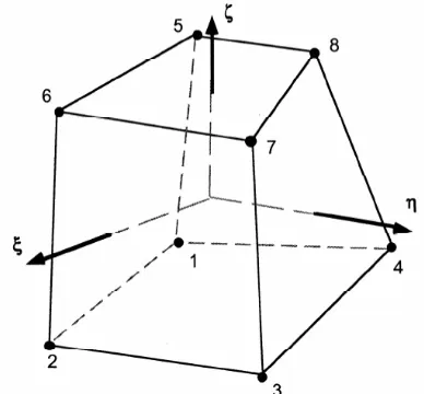
Figure 5. Eight-node Solid Hexahedron Element (Hallquist, 2006) ... 19
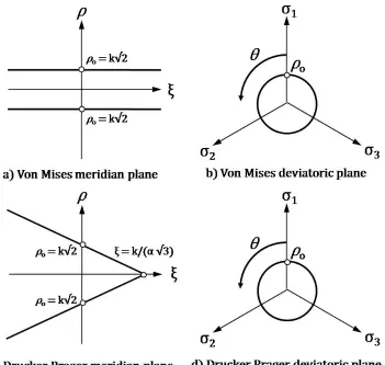
Figure 6. von Mises and Drucker-Prager Yield Surface ... 26
Figure 7. Osborn Model a) Strength b) Pressure (Johnson, et al., 2006) ... 29
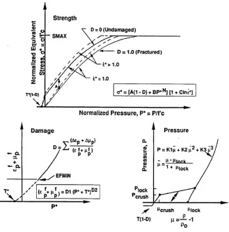
Figure 8. HJC Model (Holmquist, Johnson, & Cook, 1993) ... 32
Figure 9. BFK: a) Equation of State, b) Strength (Silling, 1997) ... 36
Figure 10. BFK Damage: Triaxial Failure Envelope (Silling, 1997) ... 38
Figure 11. K&C Strength Model a) Strength vs. Pressure, b) Typical Stress-Strain Curve (Malvar & Simons, 1996) ... 40
Figure 12. a) Deviatoric Sections of the K&C Failure Surface (Malvar & Simons, 1996), b) William and Warnke Model (Noble, Kokko, Darnell, Dunn, Hagler, & Leininger, 2005) .... 41
Figure 13. a) Shear Dilation of the K&C Model, b) Concrete Aggregate Interlock (Noble, Kokko, Darnell, Dunn, Hagler, & Leininger, 2005) ... 43
Figure 14. Typical CSCM Strength Model: a) vs. Pressure, b) Deviatoric Plane (Murray, 2007) ... 46
Figure 15. Example of Strain Softening and Modulus Reduction by Damage (Murray, 2007) ... 47
Figure 16. Experimental Setup of Impact Study ... 53
Figure 17. a) 3.0 CRH, b) 6.0 CRH Projectile Geometries in Inches (Forrestal, Frew, Hickerson, & Rohwer, 2002) ... 56
Figure 18. Relative Target Resistance with Respect to the Target-Projectile Diameter Ratio (Sjol & Teland, 2001) ... 59
Figure 19. Experimental Target Setup (Frew, 2002) ... 60
Figure 20. SNL-16 Deceleration and Example Grading System ... 70
Figure 21. Target Damage and Crater Profile for Validation ... 71
Figure 22. Example Three-Dimensional EPIC Mesh ... 75
Figure 23. Fitting of HJC Pressure Model for Low Strength Concrete ... 80
Figure 24. Example LS-DYNA Target Mesh ... 87
Figure 25. CTH Boundary Condition Diagram ... 96
Figure 26. Tecplot Output Example: a) Full, b) Zoomed ... 103
Figure 27. MPM Taylor Impact Example Results: Experimental (left)(Johnson & Holmquist, 1988) and Analytical (right)... 104
Figure 28. MPM Taylor Impact Validation Results ... 106
Figure 29. Penetration Depth for Preliminary Evaluation ... 111
Figure 33. Peak Deceleration of FEM codes for Preliminary Evaluation ... 115
Figure 34. Preliminary Evaluation Deceleration ... 116
Figure 35. Deceleration End Time for Preliminary Evaluation ... 117
Figure 36. Deceleration End Times of FEM Codes for Preliminary Evaluation ... 118
Figure 37. CPU Run Time for Preliminary Evaluation ... 121
Figure 38. Penetration Depth for Method Comparison ... 125
Figure 39. Projectile Mass Loss for Method Comparison ... 126
Figure 40. Decelerations for the Method Comparison... 128
Figure 41. Peak Deceleration for the Method Comparison ... 129
Figure 42. Deceleration Descending Slopes for Method Comparison ... 131
Figure 43. Deceleration End Times for the Method Comparison ... 134
Figure 44. HJC Low Strength Erosion Strain Determination ... 140
Figure 45. Penetration Depth for Low Strength Concrete Targets ... 141
Figure 46. Penetration Depth for Conventional Strength Targets ... 143
Figure 47. Penetration Depth with Increasing Initial Kinetic Energy for Low (LS) and Conventional Strength (CS) Concrete Targets ... 144
Figure 48. Projectile Mass Loss for Low Strength Concrete Targets ... 145
Figure 49. Projectile Mass Loss for Conventional Strength Targets ... 146
Figure 50. Projectile Mass Loss with Increasing Initial Kinetic Energy for Low (LS) and Conventional Strength (CS) Targets ... 148
Figure 51. Experimental and E-1 Comparison for Test SNL-5 ... 149
Figure 52. Peak Decelerations for Low Strength Concrete Targets ... 150
Figure 53. Peak Decelerations for Four ft. Thick Conventional Strength Targets ... 151
Figure 54. Peak Decelerations for Six ft. Thick Conventional Strength Targets ... 152
Figure 55. Peak Decelerations for Low Strength Concrete Tests with Increasing Impact Velocity ... 154
Figure 56. Peak Deceleration for Conventional Strength Concrete Tests with Increasing Impact Velocity ... 155
Figure 57. Low Strength Concrete Descending Slopes ... 156
Figure 58. Low Strength Concrete Linear Fit Descending Slopes ... 157
Figure 59. Four ft. Thick Conventional Strength Target Descending Slopes ... 158
Figure 60. Deceleration Descending Slopes for Four ft. Thick Conventional Strength Concrete Targets ... 159
Figure 61. Deceleration Descending Slopes for Six ft. Thick Conventional Strength Concrete Targets... 160
Figure 62. Linear Fit Deceleration Descending Slopes for Six ft. Thick Conventional Strength Concrete Targets... 161
Figure 63. Deceleration End Times for Low Strength Concrete Targets ... 162
NOMENCLATURE
Abbreviations and Nomenclature:
VM von Mises
JC Johnson Cook Model DP Drucker-Prager
HJC Holmquist Johnson Cook BFK Brittle Failure Kinetics K&C Karagozian & Case
CSCM Continuous Surface Cap Model EPIC Elastic Plastic Impact Calculations CTH Chart Two and a Half
MPM Material Point Method PIC Particle-in-Cell
TXC Triaxial Compression TXE Triaxial Extension
TOR Torsion
Variable Definitions:
IP Impact Pressure
P Pressure
σ Equivalent Strength, Stress
σij Total Stress Tensor
ε Equivalent Strain
εij Total Strain Tensor
E Elastic Modulus
μ Volumetric Strain
V Current Volume (Osborn) V0 Original Volume (Osborn)
Strain Rate
σT Target Strength
σP Projectile Strength
σy Yield Strength
σ1, σ2, σ3 Principal Stresses
σeq Equivalent Stress
I1 First Invariant of the Stress Tensor
J2 Second Invariant of the Deviatoric Stress Tensor
J3 Third Invariant of the Deviatoric Stress Tensor θ Angle of Similarity
φ Internal Angle of Friction
f'c Unconfined Compressive Strength (First Yield Strength for DP) f't Direct Tensile Strength (First Yield Strength for DP)
ξ Haigh–Westergaard Coordinate Representation of Pressure Influence
ρ Haigh–Westergaard Coordinate Representation of Deviatoric Stress
Normalized Equivalent Strain Rate
Pcrush Crushing Pressure
μcrush Crushing Volumetric Strain
Plock Locking Pressure
μlock Locking Volumetric Strain
σmax Maximum Equivalent Strength, Stress (Osborn)
P* Normalized Pressure T Tensile Strength
SMAX Maximum Normalized Equivalent Strength, Stress (HJC) D Damage Parameter (HJC)
Equivalent Plastic Strain to Fracture
EFMIN Minimum Equivalent Plastic Strain to Fracture Volumetric Plastic Strain to Fracture
φ Damage Rate Parameter
Y Equivalent Strength, Stress (BFK)
Ymax Maximum Equivalent Strength, Stress (BFK)
T1 Maximum Tensile Principal Stress
pref Reference Pressure
p Current Pressure
v Current Specific Volume v0 Original Specific Volume
Ω Overload
λ Shear Damage Parameter
Δλ Volumetric Damage Parameter
εv Current Volumetric Strain
εvy Volumetric Yield Strain
kd Internal Scalar Multiplier
fd Closeness Parameter
ω Associativity Parameter
θn Flow Angle for no Shear Dilation
d Damage Parameter (CSCM) ℜ Rubin Function
β Angle in Deviatoric Plane
Arbitrary Constants:
α, k, β, A, B, N, C, K1, K2, K3, D1, D2, b1, b2, b3
Mathematical Symbols:
ANALYTICAL EVALUATION OF CONCRETE PENETRATION
MODELING TECHNIQUES
1. Introduction
1.1. Background
Impact studies have traditionally focused on military applications (Zukas, 1980);
however, research interests now include that of shock compaction of powders, and modeling of void growth (Benson, 1992). Also, a developing interest has arisen for high strain rate events including collisions of automobiles, impact design for air and space vehicles, as well as processes involved in manufacturing (Benson, 1992). Zukas (1980) further includes uses for impact studies such as hazardous material transfer, nuclear structure impact design, lightweight armor design, explosive forming and welding of metals, and erosion of solids due to fluid or particle impact.
Impact and penetration of concrete involves complex material response that makes obtaining an accurate analytical solution difficult. However, compared with physical
experiments that can be financially burdensome, numerical modeling can become a practical and effective alternative (Ma & Zhang, 2007). Additionally, if conditions such as range, velocity, or impact angle outside of laboratory limits need to be studied, numerical modeling becomes necessary to further understand or predict a particular phenomenon. For these reasons, effective numerical modeling techniques are vital to the study of impact and penetration problems.
1.2. Objectives
1.3. Scope
An experimental test series performed by Sandia National Laboratories over a five month period from September 2000 to February 2001 is used as validation criteria (Rowher, Heise, & Wilder, 2001). The experimental series consisted of extensive material characterization of the target and projectile, as well as thorough data instrumentation of the impact tests. A subset of the experimental impact tests is chosen for evaluating the modeling methods and constitutive models. A single numerical approach is then applied to the entire experimental test series to further assess the code performance.
1.4. Conclusion
This document contains a survey of previous work regarding impact and penetration, modeling methods, concrete constitutive models, and available experimental data. A summation of the experimental parameters and analysis packages is presented, followed by more in depth methodology and discussion of user experience. The results of the numerical modeling software evaluation and the sensitivity study of an individual analysis
2. Literature Review
Modeling of concrete impact and penetration has many useful applications that include a range of responses and resulting phenomena. For this reason, many modeling methods and constitutive relations are continuously created and extended. The following section presents a summary of impact problems, material impact response, modeling methods, concrete
constitutive models, and available experimental data.
2.1. Definition of Concrete Impact
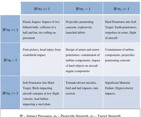
Table 1. Classification of Impact Response by Velocity (Zukas, 1980)
Striking Velocity (km/s)
Strain Rate (m/m/s)
Effect Loading
Method
>12 108 Explosive impact; colliding solids vaporize
Two-stage guns
3 – 12 107 Hydrodynamic; material
compressibility cannot be ignored
Explosive
acceleration
1 – 3 105
Materials behave as fluids; pressures
approach or exceed material strength;
density a dominant property
Powder and gas
guns
0.5 – 1 104 Viscous; material still strength significant
Powder guns
0.05 – 0.5 102 Plastic deformations Mechanical devices
Table 2. Classification of Impact Regimes by Impact Pressures and Material Strength (Wilbeck, 1985)
IP/σT << 1 IP/σT ~ 1 IP/σT >> 1
IP/σP << 1
Elastic Impact: Impact of two
billiard balls, collision of a ball and bat, tire rolling on
pavement
Projectiles penetrating
concrete, explosively launched debris
Hard Penetrator into Soft
Target: Earth penetrators, torpedoes in water, flight
of aircraft
IP/σP ~ 1
Fruit pickers, head injury from windshield impact
Design of armor and armor penetrators, containment of
turbine components, impact
of hard objects on aircraft
engine components
Containment of turbine components, projectiles
penetrating concrete
IP/σP >> 1
Soft Penetrator into Hard
Target: Birds impacting
aircraft canopies at low flight
velocity, lead bullets
impacting a steel plate
Tornado-driven missiles,
bird and hail impacts, rain
erosion
Significant Material
Failure: Hypervelocity
impacts,
IP – Impact Pressures,σP – Projectile Strength, σT – Target Strength
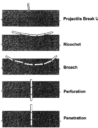
Figure 1. System Response (Cargile D. , 1998)
and penetration. Perforation is the complete piercing of a target by a projectile, whereas penetration is entrance of a projectile into a target without complete passage (Zukas, 1980). These two processes result in large deformations in both projectile and target. Availability of research into projectile ricochet and broach are limited possibly due the difficulty of safe experimental control and data collection.
2.2. Modeling Techniques
Analytical techniques of projectile penetration analysis are empirical equations, analytical models, and numerical methods (Cargile D. , 1998; Jonas & Zukas, 1978). Of these methods the most detailed level of analysis is numerical methods; the techniques in this section will be focused on numerical methods used in impact modeling. Numerical methods can be
characterized by three essential aspects involved in any simulation: kinematic description, discretization, and solution method.
2.2.1. Kinematic Descriptions
methods. Of these additional methods, only Arbitrary Lagrangian Eulerian (ALE) and meshless methods will be presented in this section.
2.2.1.1. Lagrangian
Lagrangian methods use dynamic grids to follow the distortion of materials. The
governing conservation equations are solved on the deformed mesh at discrete points in time. Cells are only allowed to contain individual materials; they cannot contain a mix of multiple materials. This trait requires slide lines or contact definitions to handle material contact. For a particular cell in a Lagrangian point of reference, mass remains constant throughout
computation, but the volume is allowed to change due to extension or compression of the material. Lagrangian analysis programs have grown in popularity and are commonly selected for modeling collision and manufacturing problems (Benson, 1992). LS-DYNA is a
2.2.1.2. Eulerian
Eulerian methods use a stationary mesh through which material is advected. The flow into and out of a fixed cell is used to calculate new values for field variables in that cell. While early implementation of Eulerian methods involved mass particles, most modern versions use continuous materials. CTH (Crawford, et al., 2007) is a popular Eulerian code (Mair, 1999), and has been frequently employed for impact research (Senft & Stewart, 2007; Donea, Huerta, Ponthot, & Rodriguez-Ferran, 2004). Eulerian methods present great
advantages in models with large deformation due to their ability to capture this behavior without a deformed mesh. Impact modeling with Lagrangian techniques often requires remeshing or erosion algorithms to maintain numerical stability; this can be avoided with an Eulerian frame of reference. Because the mesh is stationary throughout calculation, Eulerian cells are allowed to contain multiple materials. This mixing of materials in cells can present difficulties in modeling material and boundary interfaces. One improvement often
2.2.1.3. Arbitrary Lagrangian-Eulerian
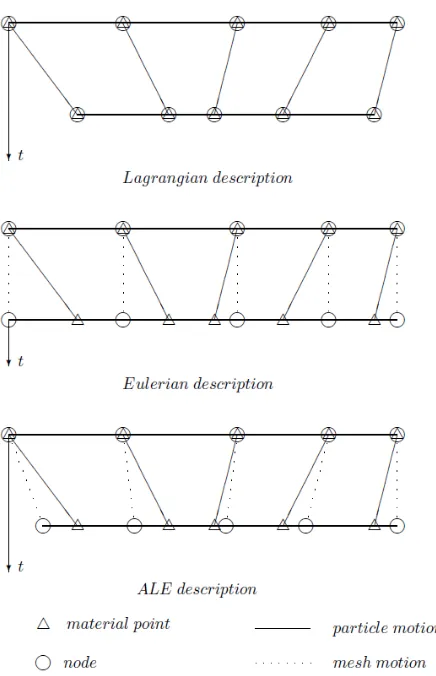
The most well known extension of the Lagrangian and Eulerian methods is the Arbitrary Lagrangian-Eulerian method. Developed to combine advantages and minimize limitations of Lagrangian and Eulerian methods, ALE maps the solution to a dynamic mesh independent of material motions or spatial coordinates. This mesh is allowed to remain fixed like Eulerian methods, follow the material distortion like Lagrangian methods, or move arbitrarily (Donea, Huerta, Ponthot, & Rodriguez-Ferran, 2004). This flexibility enables ALE codes to capture large deformations while maintaining clear interface distinctions. Figure 2 illustrates
Figure 2. Comparison of Lagrangian, Eulerian, and ALE Descriptions (Donea, Huerta, Ponthot, & Rodriguez-Ferran, 2004)
A simplified implementation of the ALE method is provided in the 2006 version of LS-DYNA which allows for automatic rezoning to stabilize calculations with large deformations (Hallquist, 2006); ALE methods like this one provide second order accurate solution
garnered ALE methods much interest and use in problems of fluid and structural dynamics including situations involving impact and penetration (Donea, Huerta, Ponthot, & Rodriguez-Ferran, 2004). However, ALE codes typically involve higher computational costs per
element than other methods, and these costs vary depending on remapping algorithms and whether or not the method allows more than one material per cell (Benson, 1992).
2.2.1.4. Meshless Methods
great potential to model history dependent materials in problems with large distortions without highly distorted meshing or difficulties of material boundaries and cell mixing.
2.2.1.5. Kinematic Description Summary
Lagrangian methods have been popular for structural mechanics problems, especially in static problems. However, with increased material interaction the Lagrangian point of reference can become highly distorted and unstable. Eulerian methods have been more common in the field of fluid dynamics, but face difficulties in material interface descriptions in structural problems. ALE methods are coupled Lagrangian and Eulerian methods that have shown improved modeling, but incur higher computational costs. Meshless methods
represent efforts to move from the limitations associated with all meshed techniques; these methods are still early in development but show promise. While each of these kinematic description methods has potential areas of difficulty, all present capable means of modeling impact and penetration problems.
2.2.2. Discretization Methods
approximate the governing differential equations while engineers created relations between actual discrete elements and finite sections of a continuum domain. These methods of discretization have been developed simultaneously and interdependently. (Zienkiewicz, 1979)
Finite difference and finite element methods now represent two popular numerical approximations used to model partial differential equations involved in continuum problems (Anderson, 1987). The major difference between most finite element and finite difference programs used in impact and penetration applications is the method used to calculate accelerations and their associated forces, while the equations to update the stresses, energy, and shock viscosity are equivalent (Benson, 1992). In implementation, finite element
methods employ segmented ordinary polynomial equations to approximate partial differential equations where finite difference codes employ differencing equations.
2.2.2.1. Finite Element Method
The Finite Element Method (FEM) is a numerical technique that provides approximations of partial differential equations. FEM approximates a fully continuous solution by a
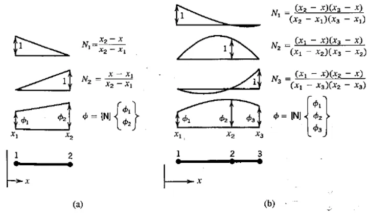
interpolation schemes, consider “Lagrange’s interpolation formula” shown in Figure 3; where is the shape function corresponding to the node at for number of nodes along the coordinate . The figure shows linear (a) and quadratic (b) interpolation regarding the field variable . FEM applications can provide convergent solutions in analysis programs and are commonly used in many types structural mechanics applications. (Cook, Malkus, Plesha, & Witt, 2002)
Figure 3. Lagrange Interpolation and Shape Functions: a) Linear, b) Quadratic (Cook, Malkus, Plesha, & Witt, 2002)
2.2.2.1.1. Element Type
FEM programs offer a number of elements to choose from, but avaiablilities differ between codes. To illustrate the importance of element type selection, consider two common two-dimensional elements that meet commonly accepted FEM robustness requirements: the linear, constant strain triangle (CST) and the bilinear quadrilateral (Q4). Because of the linear deformation and resulting constant strains across the element, the CST exhibits slow
convergence, spurious shear, and excessive stiffness in bending and even demonstrates erroneous locking in plane strain conditions (Cook, Malkus, Plesha, & Witt, 2002). The Q4 is unable to model pure shear because it experiences shear locking behavior due to parasitic shear (Cook, Malkus, Plesha, & Witt, 2002). While both the CST and Q4 meet the
fundamental robustness requirements of continuity, compatablity, and completeness, both exhibit inherent inaccuracies.
In current three-dimensional FEM programs, tetrahedral and hexahedron (brick) elements are commonly used. Johnson et al. (2006) recommend using tetrahedral elements in a
modes (Hallquist, 2006); however, potential hourglassing modes may occur that must be prevented by viscous damping or the recommended elastic stiffness method. Figure 4 and Figure 5 show typical tetrahedral and hexahedron elements.
Figure 5. Eight-node Solid Hexahedron Element (Hallquist, 2006)
Elements used in FEM analyses range in complexity and efficiency. The most effective element may depend on the particular application or FEM code. The CST and Q4 two-dimensional elements serve as an illustration that elements common to finite element codes must be cautiously selected in order to avoid discretization error.Whatever the application or analysis code, much attention should be paid to the choice of element type to avoid erroneous results.
2.2.2.2. Finite Difference Method
differencing equations are employed to replace the partial derivatives in differential equations inherent with continuum solutions. Forward, backward, and central difference equations are examples of FDM approximations for the derivatives of a continuous function. FDM represents the differential equation solution with pointwise descriptions of the discrete system that exhibit minimal computational cost and are typically easier to implement than FEM algorithms. Despite offering less accuracy than FEM, the ease and efficiency of FDM approximations have made them popular in applications of computational fluid dynamics where problems can involve discretizations on the order of a million or more grid cells. (Smith, 1985)
2.2.2.3. Discretization Summary
FEM and FDM represent two prominent discretization techniques currently used. The differences between the two approaches have reduced significantly over years of
has been shown that in solid dynamic problem sizes where it remains computationally effective, FEM analyses provide more robust solutions (Cook, Malkus, Plesha, & Witt, 2002).
2.3. Constitutive Models
Numerical methods require constitutive relationships that describe the physical response of each of the materials involved in the analysis. Constitutive models vary in complexity and require laboratory testing for material property data (Babu, Benipal, & Singh, 2005). Material models used in impact and penetration analysis must describe physical observations of
material response. Inaccuracies with constitutive models largely limit numerical methods and deserve greater attention especially when considering impact at ordinance velocities where the material strengths dominate the response (Jonas & Zukas, 1978).
Concrete constitutive models for numerical methods have improved in the last 40 years based upon the ability to capture accurate material response from experiments (Babu, Benipal, & Singh, 2005). Material models for concrete have historically been classified into numerous approaches including elasticity, plasticity, and inelasticity theories. More recently fracturing, continuum damage, and microplane models have appeared in the literature. Two common categories of concrete modeling are plasticity models and continuum damage models. While plasticity models do not form the majority of current material relations used for brittle geomaterials, they represent a large portion of previous literature in constitutive modeling and form a basis for material models used currently. Continuum damage models represent a larger portion of concrete material models used in current numerical methods.
2.3.1. Plasticity Models
relation of more recent continuum damage models. The Osborn model will also be discussed though it would not be defined as a classical plasticity model. However, it does represent a connection of current continuum damage models with the theory of plasticity.
2.3.1.1. von Mises
The von Mises yield criterion is one of the earliest pressure independent plasticity
models. The yield criterion or yield function, f, is defined by a critical yield stress, σy, and the
second invariant of the deviatoric stress tensor, J2, which is defined by the stresses in the
principle directions, σ1, σ2, and σ3:
Equation 2.1
where Equation 2.2
It is helpful to note that, in the plasticity models and continuum damage models discussed
here, strength is defined as an equivalent stress, σeq, or von Mises stress ( ):
Equation 2.3
This equivalent stress can also be described as shear strength or principle stress difference, τ, in terms of axial stress ( ) and radial stress ( ) of a concrete cylinder under axial compression with or without confinement (Hanchak, Forrestal, Young, & Ehrgott, 1992):
The yield function, interpreted visually as a failure surface, can be defined as an elastic limit of the equivalent stress. The von Mises yield criterion laid the foundation for future concrete plasticity models; however it was developed and designed for materials whose strength was unaffected by confining pressure. This has not been found true for concrete (Ashby &
Hallam, 1986; Joy & Moxley, 1993; Cargile D. , 1998), therefore von Mises is inadequate for concrete modeling.
2.3.1.2. Drucker-Prager
Drucker-Prager is a two-parameter plasticity yield criterion that represents a pressure dependent extension the von Mises yield criterion (Chen & Han, 1988). The Drucker-Prager function includes the first invariant of the stress tensor, referred to as :
Equation 2.5 which allows for the influence of pressure on the strength of the material. The influence of pressure is important and can be observed in concrete testing; the addition of pressure by confinement in an axial compression test results in greater observed strengths.
The Drucker-Prager yield criterion takes the form:
, Equation 2.6 where and are arbitrary material constants. A possible definition for the and
and Equation 2.7
where Equation 2.8
Figure 6. von Mises and Drucker-Prager Yield Surface
The meridian plane represents a comparison of a quantity of deviatoric stress, ρ, to a quantity of hydrostatic stress, ξ; these terms are expressed:
The angle of similarity, θ, represents differences between compressive and tensile meridians. Implementation of the Drucker-Prager model requires a hardening rule and a flow rule to define plastic deformation. Hardening rules require that material constants, and , be variable functions of a hardening parameter which is often defined by a hardening modulus applied to the elastic-plastic equations. Commonly, the flow rule is formed by replacing the parameter with a material dilatancy constant, . If is greater than 0, plastic deformation will result in volume increase. If is equal to , the flow rule is said to be associative which assumes the material is elastic-perfectly plastic; this is not commonly assumed for concrete, and terms for range between zero and (Loret & Prevost, 1986).
Of the plasticity models, Drucker-Prager is one of the more basic pressure dependent models with constants that are easily determined from compression and tension tests. While Drucker-Prager has been frequently used for modeling soils in the past, the model exhibits deficiencies in modeling concrete because it includes a simple linear relationship between ρ and ξ, as well as no effect by the angle of similarity, θ, resulting in undesired similarity
accurate concrete modeling; in current literature, Drucker-Prager is only an adequate concrete representation in limited loading cases where materials remain in the elastic range (Loret & Prevost, 1986; Lopez-Cela, 2002).
2.3.1.3. Osborn (Hull)
Figure 7. Osborn Model a) Strength b) Pressure (Johnson, et al., 2006)
The equation of state, or pressure model, is used to characterize the high pressure,
impulsive loading present in high velocity impact (Cargile D. , 1998). Volumetric strain, μ, is a representation of the multi-dimensional deformation of the concrete and is defined in terms of relative volume, V0/V, as shown in Figure 7 b). The equation of state is defined in three
sections: elastic (prior to the crushing point), crushing (between the crushing and locking points), and locking (where all voids are assumed removed). These sections rely on the definitions of the curve fitting constants, K1, K2, and K3, as well as the crushing point
(defined by Pcrush and μcrush) and locking point (defined by Plock and μlock).
of strain rate on the concrete strength, it neglects the accumulation of damage. Validation work for this concrete model is limited and difficult to access. The Osborn concrete model represents an extension of plasticity theory towards decoupled deviatoric and volumetric response; and while validation of the model is scarce, it does present potential advances in concrete modeling.
2.3.2. Continuum Damage Models
While plasticity theory models have been implemented with a level of accuracy in the past, they are highly dependent on the assumption of a well defined yield surface which can be difficult to specify in concretes. Concrete response beyond the elastic limits is based largely on the growth and spread of microcracks (Cargile D. , 1998), and recent work has been devoted to the incorporation of cumulative damage on the strength of brittle
2.3.2.1. Holmquist Johnson Cook Concrete (HJC)
As an expansion of the Osborn model, the HJC model contains a strength relation and equation of state similar Osborn; however, HJC introduces features to better model concrete penetration by considering large strains, high strain rates and high pressures (Holmquist, Johnson, & Cook, 1993). Among these improvements, HJC incorporates the effects of cumulative damage and complete crushing of concrete at high pressures (Figure 8).
The strength portion of the model is nonlinear and defined by normalized equivalent stress, *, versus normalized pressure, P*, both normalized by the unconfined compressive strength, f’c. A damage parameter, D, is applied to the cohesive strength constant, A, which represents the difference between undamaged and fractured strength. Other strength
constants include the normalized pressure hardening coefficient and exponent, B and N, respectively, as well as the strain rate constant, C, and the normalized maximum strength, SMAX. The tensile portion of the strength curve is determined by a normalized tensile strength constant, T*, with damage applied.
The equation of state contains the three regions as described in the Osborn model: elastic, crushing, and locking. The three regions are segmented by the crushing and locking points. In HJC, the crushing region is considered linear and the locking portion is a normalized polynomial. The curve also contains a triaxial tension region based on the direct tension constant, T, with damage applied. As an alternative to modifying all the constants to fit the curve to hydrostatic compression test data, formulas are given for all of the constants in the equation of state except for T, Plock, K1, K2, and K3 which are used to fit the model to data.
equal to one. Notice that as pressure increases more plastic strain is required to reach a damage value of one. This description of damage considers a behavior that can be seen in triaxial compression tests; with higher confining pressures the strain at failure increases. The damage model contains material constants T*, D1, D2, and EFMIN which are selected as the
values recommended in the original work. (Holmquist, Johnson, & Cook, 1993)
As an extension of the Osborn model, HJC introduces additional capacity to represent concrete response and requires additional work to implement the model for a specific
concrete. The HJC model contains a large number of material constants compared to simpler plasticity models; however, for many of these constants suggested formulas are given or recommended values are provided to ease implementation. Numerous material tests are required to completely define the constants for a particular concrete specimen. The strength model requires an unconfined compression test, a direct-pull test, a series of triaxial
Perry, 1986; Hughes, Tedesco, & Ross, 1993; Ross, Kuennen, & Tedesco, 1992). While the introduction of cumulative damage provides a promising link between elastic and completely crushed concrete, the model representation of damage is limited. For example, triaxial test data shows the strength difference between undamaged and fractured concrete is reduced as confinement levels are increased; this indicates that the cohesive strength constant, A, should be variable, influenced by pressure. Similarly, the damage constant, D2, which can show
lower damage accumulation with higher pressures is commonly assigned a value of one following the work of Holmquist et al. (1993); this implies that failure strain and pressure are directly proportional. Triaxial test data from other literature has not supported this theory (Ashby & Hallam, 1986; Joy & Moxley, 1993; Cargile D. , 1998). Much HJC validation work has focused on the perforation of concrete. The model has shown adequate results for reinforced concrete (Holmquist, Johnson, & Cook, 1993; Tai & Tang, 2006), but other sources have highlighted the existance of deficiencies at high velocities (Dawson, Bless, Levinson, Pedersen, & Satapathy, 2008). Wang et al. found HJC to be inadequate for modeling tensile fracture and spallation craters (2007). Polanco-Loria et al. made
2.3.2.2. Brittle Failure Kinetics (BFK)
The Brittle Failure Kinetics model was developed to represent concrete response in problems involving penetration and large stress waves. The model is based on rate effects applied through a time dependent damage variable. BFK employs Mohr-Coulomb failure curves to describe strength and an equation of state to relate pressure and density. The model seperates itself from other rate dependent concrete models in that strain rate is not explicitly included, but treated by a delay time, ‘time to failure’ (Silling, 1997).
Figure 9. BFK: a) Equation of State, b) Strength (Silling, 1997)
The strength model is used to define the yield strength in a manner similar to that used in plasticity theory. Mohr-Coulomb strength surfaces and a scalar damage parameter, φ, are
strength curves are shown as straight lines on the plane of yield strength, Y, versus maximum negative principal stress, T1, positive in tension. The equation of state for the BFK model is
defined by pressure and internal energy density reference curves (Silling, 1997). The pressure reference curve (compression) is fit to shock Hugoniot data by specific volume, v, and
pressure, p, value pairs. The model distinguishes between loading and unloading due to the nature of void compression in concrete by the inclusion of a separate release curve as shown in Figure 9 a). The BFK damage variable, φ, is defined by the summation of brittle, ductile,
and compressive damage rates and is dependent upon rate and geometry. Figure 10 shows the difference between an ideal strength surface and a typical triaxial failure envelope. The failure envelope does not follow the strength surfaces because the envelope includes damaged states. A separate failure surface exists for each value of φ between zero and one.
To help describe the rate dependent response, Silling defined Ω as the ‘overload’, shown in
Figure 10. BFK Damage: Triaxial Failure Envelope (Silling, 1997)
The BFK model presents an alternative method for incorporation of rate dependent damage in concrete modeling. BFK provides the capacity of accurately modeling concrete with the cost of more rigorous implementation requirements for specific modeling. Unlike HJC, implementing the model for a specific concrete specimen is not described. Certain testing requirements are implied and means of proportioning data to previously implemented materials are given. The strength model would require compressive testing with multiple confinement levels and tensile testing to determine the curve intercepts with the T1 axis. The
The representation of damage in terms of rate is a potentially useful method in modeling observed responses of concrete under impulse loads over short durations, specifically like those characteristic of concrete impact. Silling performed initial validation analyses for concrete penetration using BFK (1997) and found the model to perform well when inspecting impact velocity (400 to 1000 m/s) and penetration depth (30 to 1100 cm). The model also exhibited accurate modeling of decelerations of the projectiles perforating concrete. However, the BFK model has shown deficiencies with regard to spalling and late-time damage in concrete perforation simulations involving impact velocities on the order of two km/s (Dawson, Bless, Levinson, Pedersen, & Satapathy, 2008). The BFK model provides a promising means of modeling complicated concrete response with alternative methods for considering the strength relation, strain rate effects, and damage.
2.3.2.3. Karagozian & Case (K&C)
Figure 11. K&C Strength Model a) Strength vs. Pressure, b) Typical Stress-Strain Curve (Malvar & Simons, 1996)
The two major features in this strength model are the distinction between the yield, maximum, and residual failure surfaces and the inclusion of the third invariant of the deviatoric stress tensor, J3, which is proportional to the similarity angle, θ. The strength
influence of the third invariant on the failure surface in three-dimensional stress space can also be observed in Figure 12 a).
Figure 12. a) Deviatoric Sections of the K&C Failure Surface (Malvar & Simons, 1996), b) William and Warnke Model (Noble, Kokko, Darnell, Dunn, Hagler, &
Leininger, 2005)
The intricate three invariant surface requires that the three failure surfaces be fit to concrete material tests using eight material constants determined by triaxial compression data. A direct tensile strength is required to proportion the tensile meridians of the model.
The K&C model includes shear and volumetric damage. The shear damage parameter of
the model, λ, involves strain rate enhancement (rf), pressure (p), effective plastic strain ( ),
where Equation 2.10
The rate enhancement factor is a user defined parameter that can be modeled by an input table. In order to include damage in triaxial tension the volumetric damage, Δλ, must be included; it involves current volumetric strain, εv, volumetric yield strain, εvy, an internal
scalar multiplier, kd, material constant, b3, and a closeness parameter, fd, that describes how
close the stress state is to triaxial tension and is based on the second invariant of the stress tensor, J2:
Equation 2.11
where Equation 2.12
The damage variables are used by the strength model to interpolate the updated strength between the three failure surfaces of the strength model using a relation between the damage and the effective strength ratio, η, ranging from zero at yield strength to one at maximum strength and back to zero at residual strength. To implement the damage model for a concrete material the three material constants b1, b2, and b3 must be determined in addition to a tabular
relation between the λ and η.
a) illustrates the use of an associativity parameter, ω, to implement partial shear dilation of concrete caused by aggregate interlock; suggested values of ω range from 0.5-0.7 (Noble,
Kokko, Darnell, Dunn, Hagler, & Leininger, 2005). Additionally, the maximum width of the concrete aggregate is required to model the material flow.
Figure 13. a) Shear Dilation of the K&C Model, b) Concrete Aggregate Interlock (Noble, Kokko, Darnell, Dunn, Hagler, & Leininger, 2005)
user defined equation of state allows for flexibility, but may introduce unwanted user error. A drawback with the damage implementation is in the area of confining pressure; no distinction is made for stress-strain curves of different confinement levels (Yonten, Manzari,
2.3.2.4. Continuous Surface Cap Model (CSCM)
Cap models represent a recent development trend in continuum damage models for concrete. With the earliest work appearing in the late 1970s by Isenberg, Vaughan, and Sandler (1978), the cap model is based on the idea that continued hydrostatic loading will yield concrete material. A more recent implementation, the CSCM model, evolved from a strain sub-incrementing method by Pelessone (1989) and extended the earlier cap
implementation known as the Geological Cap Model that neglected the third stress invariant, damage, and strain rate effects (Hallquist, 2006). The CSCM model was originally developed for defense purposes in the analysis of dynamic loading of reinforced concrete structures in the early 1990s under the various titles including ‘Single Surface’, ‘Smooth Cap’, and ‘Schwer-Murray’ (Schwer & Murray, 1994). More Recently the CSCM has been
Figure 14. Typical CSCM Strength Model: a) vs. Pressure, b) Deviatoric Plane (Murray, 2007)
The CSCM strength model uses an ultimate failure surface which combines both shear failure and cap hardening (Figure 14 a). The strength model includes an ability to describe the pre-peak nonlinearity in concrete stress-strain curves involving low confinement levels. Figure 14 shows that the Rubin scaling function is incorporated in the strength model to represent the effects of the third invariant of the deviatoric stress tensor, , which is directly
concrete pressure-volumetric strain response or equation of state. CSCM incorporates damage applied in two forms: strain softening and modulus reduction by applying a scalar damage parameter, d, varying from zero to one, to the undamaged stress tensor. The effect damage has upon strain softening and modulus reduction is shown in Figure 15.
Figure 15. Example of Strain Softening and Modulus Reduction by Damage (Murray, 2007)
CSCM involves a strength failure surface, damage accumulation, and strain rate effects. The model considers many of the responses of concrete in a range of pressure levels and triaxial stress states. Because CSCM was developed for a time sensitive application for the roadside safety community, ease of use was an important consideration for the developers. The model has up to 37 inputs parameters, with a minimum of 19 that must be fit to
experimental data for the concrete. However, with the limitations of time, data, and material modeling expertise in mind, the model includes provisions for standardized material
2.3.3. Constitutive Models Summary
Classical plasticity models represent early efforts to model the yield and flow of
materials; however, in high strain rate, impulsive loading conditions these plasticity models fail to capture experimentally observed material responses. Plasticity models have been extended in many of the common continuum damage models for concrete in order to
incorporate more of the complex responses of brittle materials under impulse loads extending beyond elastic limits. These continuum damage models show many improvements from the classical plasticity methods by including effects of strain rate, damage, and confining pressures. The continuum damage models can require rigorous efforts for implementation, and the selection of an appropriate material model for analysis may become a balance between experimental data availability and model capacity to capture material response.
2.4. Available Experimental Work
penetration, perforation, and detonation testing. Table 3 presents a survey of concrete case studies.
Table 3. Concrete Impulse Loading Case Studies
Author(s) Projectile Length (in) Projectile Mass (lb) Impact
Velocity (ft/s) Target Type Test Type
Forrestal et al.(2002) 20.7 28.66 459-1509 Unreinforced Penetration Cargile(1998) 9.54 1.98 909-2625 Unreinforced Penetration Cargile, Tidwell(1993) 14 5.16 801-1499 Unreinforced Normal and Oblique Penetration Dancygier et al.(2007) 7.83 3.31 656-1033 Reinforced Penetration Gold et al.(1996) 2.95-7.48 0.35-0.88 4921-6233
reinforced and
unreinforced Penetration Unosson,
Nilsson(2006) 8.86 13.89 2011-2047 reinforced and unreinforced
Penetration and Perforation Dawson et al.(2008) 3.72 0.114 4888-7415 reinforced and unreinforced Perforation Averett et al.(2005) 20.77 29.19 984 unreinforced Perforation Hanchack et al.(1992) 5.66 1.1 984-3609 Reinforced Perforation Cargile et al.(1993) 14 5.16 1014-1552 Unreinforced Perforation Ehrgott et al.(2007) - C4, 4.23-8.82 - Reinforced Detonation Akers et al.(2005) - C4, 9.92 - Reinforced Detonation Akers et al.(2003) - C4, 9.92-13.67 - Reinforced Detonation Malvar, Simons(1996) - Class 1.1, 272 - Reinforced Detonation
Both fields of study have only recently begun to consider projectile erosion, deceleration, and target crater profiles. Detonation testing commonly considers only crater width and profile, and is focused on targeting and weaponeering applications. These experimental studies involving high strain rate, impulsive loading provide valuable observations of material responses that can be used to develop and validate modeling methods and material models.
2.5. Need for Research
Concrete impact and penetration is a complex phenomenon. The nature of concrete response presents particular complexities, especially under loads of highly impulsive pressures over short durations. Much work has been done to improve modeling methods of this problem, and currently there are numerous techniques and constitutive models available exhibiting promising and accurate results. The continued development of numerical analysis methods can offer an invaluable resource to study these phenomena; however, validation and verification through experimental testing is required.
Research is needed to further understand and characterize response of concrete to impact and provide data necessary to refine and validate current analysis methods.
The current research will compare common modeling packages and constitutive models and provide a validation study for their use in concrete impact and penetration, as well as
3. Basic Problem
Figure 16. Experimental Setup of Impact Study
This research will compare the analytical results from multiple concrete constitutive models and analysis packages to experimental data to assess performance for concrete impact and penetration scenarios. The modeling of these problems requires understanding of 1) the material properties and geometry of the projectile, 2) the material details and dimensions of the target, and 3) the impact conditions including impact velocity, angle of inclination, and target constraints (Cargile D. , 1998). These three parts of the validation impact experiment, summarized in Figure 16, must be well understood and appropriately applied to each
3.1. Experimental Data
Table 4. Experimental Test Matrix (Forrestal, Frew, Hickerson, & Rohwer, 2002)
Test Name
Concrete Target Projectile Penetration
Depth Type
Strength Thickness Nose Shape
Velocity Obliquity (degrees)
(ksi) (ft) (ft/s) Pitch
(Up/Down)
Yaw
(Left/Right) (in)
SNL-00-11 Conv. Str. 5.7 4 3.0 CRH 781 0.1D 0.0 11.8 SNL-00-12 Conv. Str. 5.7 6 3.0 CRH 904 0.1D 0.4L 15.0 SNL-00-09 Conv. Str. 5.7 4 3.0 CRH 1030 0.2D 0.2R 17.7 SNL-00-10 Conv. Str. 5.7 4 3.0 CRH 1212 3.6U 2.5L 20.9 SNL-00-14 Conv. Str. 5.7 6 3.0 CRH 1497 0.2U 0.2R 37.0 SNL-00-15 Conv. Str. 5.7 6 6.0 CRH 1025 N/A N/A 24.0 SNL-00-16 CSPC 5.7 6 6.0 CRH 1471 0.5U 0.2R 39.0 SNL-00-06 Low Strength 3.3 6 3.0 CRH 457 0.3D 0.2L 9.4 SNL-00-03 Low Strength 3.3 6 3.0 CRH 658 0.0 0.4L 16.5 SNL-00-02 Low Strength 3.3 4 3.0 CRH 820 0.4D 0.3R 24.4 SNL-00-01 Low Strength 3.3 4 3.0 CRH 931 0.2U 0.4L 29.9 SNL-00-05 Low Strength 3.3 6 3.0 CRH 1104 0.2U 0.1R 36.6 SNL-00-04 Low Strength 3.3 6 3.0 CRH 1242 0.3U 0.2R 46.5 SNL-00-08 Low Strength 3.3 6 6.0 CRH 782 0.5D 0.3R 22.8 SNL-00-07 Low Strength 3.3 6 6.0 CRH 1242 0.0 0.6L 49.2 3.1.1. Projectile
The projectiles in the experimental test series were constructed of 4340 RC45 steel and
Figure 17. a) 3.0 CRH, b) 6.0 CRH Projectile Geometries in Inches (Forrestal, Frew, Hickerson, & Rohwer, 2002)
density and projectile voids were modeled so that the weight and center of gravity of the projectiles matched the experimental test projectiles.
3.1.2. Target
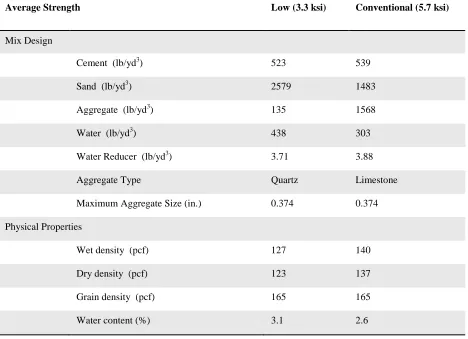
The targets in the experimental test series varied in thickness and concrete strength. The targets were constructed by casting concrete into corrugated steel pipes six ft. in diameter, and allowed to cure for at least 140 days. Four ft. and six ft. target thicknesses were used in testing. The target concretes consisted of low-strength (3.3 ksi) and a conventional-strength (5.7 ksi) concrete; the unconfined compressive strengths were determined on the testing date, 140 or more days after the pour, unlike the 28 day test common to civil engineering practice. Table 5 provides detailed material descriptions of the experimental concretes. Further
Table 5. Mix Design and Properties of the Experimental Concrete (Forrestal, Frew, Hickerson, & Rohwer, 2002)
Average Strength Low (3.3 ksi) Conventional (5.7 ksi)
Mix Design
Cement (lb/yd3) 523 539
Sand (lb/yd3) 2579 1483
Aggregate (lb/yd3) 135 1568
Water (lb/yd3) 438 303
Water Reducer (lb/yd3) 3.71 3.88 Aggregate Type Quartz Limestone
Maximum Aggregate Size (in.) 0.374 0.374
Physical Properties
Wet density (pcf) 127 140
Dry density (pcf) 123 137
Grain density (pcf) 165 165
Water content (%) 3.1 2.6
concrete cylinders in compression testing (Ashby & Hallam, 1986; Joy & Moxley, 1993; Cargile D. , 1998). However, Sjol and Teland (2001) have shown that in impact testing the boundary effects of steel confinement significantly reduce as the ratio of target to projectile diameter, dt/d, approaches 25 in./in. (Sjol & Teland, 2001), illustrated in Figure 18. Sjol and
Teland conclude that analytical and experimental work indicate confining boundary effects can be neglected for tests involving target to projectile diameter ratios beyond 15 . In the validation impact tests used in this research, the target-projectile diameter ratio equals 22.5.
3.1.3. Initial and Boundary Conditions
The initial and boundary conditions in the validation experiments include the velocity and angle of the projectile at impact as well as the restraint placed on the targets during the
impact event. The impact tests were conducted by launching the projectiles horizontally from a 3.27 in. diameter powder gun at varying velocities from 456 to 1497 ft/sec. While the test setup was structured in a way to avoid oblique impacts, slight inclination angles did exist upon projectile impact. These inclination angles, captured by high speed digital photographs, were recorded in the experimental data and applied in the analyses. The concrete target contained in the corrugated steel was placed in a carriage restraint for the experimental impact tests; this restraint is described by the diagram in Figure 19.
For the analytical calculations the effect of gravity on the problem is neglected due to the short length of time over which the event takes place, less than six milliseconds. The
interaction of gravity on the event is small relative to the forces caused by impact. For all codes with available options, the angles at impact were included and the carriage restraint was modeled consistent with the experimental tests.
3.2. Analysis Methods
Concrete material models and analysis code pairings were evaluated on their ability to reproduce specific concrete penetration results as well as available output and CPU run time. Analysis codes of different foundational backgrounds will be included in this work, and certain concrete constitutive models available in the analysis codes will be used.
3.2.1. Material Models
has been shown to be an adequate representation of metals (Johnson and Holmquist, 1988) and is available in three of the four modeling programs used in this research. A simpler von Mises plasticity model is used where the JC model is unavailable.
Five commonly available concrete material models will be evaluated due to the direct influence concrete model response has on the accuracy of the modeling program. The Drucker-Prager, Osborn, Brittle Failure Kinetics, Holmquist Johnson Cook and Karagozian & Case concrete models were selected based on code availability and popularity.
3.2.2. Analysis Packages
The four analysis packages compared in this research represent a cross-section of both popular and promising techniques. Two Finite Element Method (FEM) analysis programs are considered in this work, EPIC and LS-DYNA. A third program, CTH, is a Finite Difference Method (FDM) code. The final analysis option is the Material Point Method (MPM)
implemented in a two-dimensional FORTRAN code.
3.2.2.1. EPIC
EPIC stands for Elastic Plastic Impact Calculations. For this reason, EPIC contains many useful material models common to projectiles and structural targets as well as useful design features for contact, boundary conditions, and erosion (Johnson et al. 2006). For this
research, the three-dimensional tetrahedral modeling method in EPIC is used for evaluation.
3.2.2.2. LS-DYNA
LS-DYNA development has focused on the analysis of structural impact and impulse loading. Evolving from DYNA3D, developed in 1976, LS-DYNA is the commercial version of the software from Livermore Software Technology Corporation (Hallquist, 2006). Version 971 released in 2007 is used in this research. LS-DYNA provides an extensive library of material models, contact options, and other features (Livermore Software Technology Corporation, 2007). While LS-DYNA offers a wide variety of solution types useful for impact and penetration, for the purpose of evaluation, the three-dimensional finite-element hexagonal modeling method is used in the analysis.
3.2.2.3. CTH
phase in solving the governing equations while deformations are not large (Crawford et al., 2007). Version 8.1 released in 2007 is used in this research. CTH provides a range of models for materials common to impact as well as several advanced features including adaptive mesh refinement. For the purpose of this evaluation, the standard three-dimensional finite difference solution is selected for analysis. Due to the nature of the fixed mesh in Eulerian methods, difficulties were encountered applying the saddle boundary constraint as a curved surface. As an alternative, a simpler tangential boundary condition was applied to the target.
3.2.2.4. MPM
MPM is an ALE code implemented in FORTRAN by Allen York, Shijian Zhou, and Deborah Sulsky at Sandia National Laboratories (York et al., 1997). It is a research code and not commonly available. MPM has shown potential for improving upon the more common Lagrangian and Eulerian methods, especially in impact and contact problems. Contact between different materials is handled inherently. While still in the developmental stages, MPM provides a limited number of constitutive models and options. This method is limited to a two-dimensional version at this time; hence a cylindrically symmetric boundary
3.2.3. Summary of Packages and Models
Table 6. Analysis Matrix for Target Material Models Analysis
Program
Target Material Model
DP HJC KC Osborn BFK
EPIC E-1 E-2 LS-DYNA
L-1 L-2
CTH C-1 C-2 MPM M-1
DP - Drucker-Prager, HJC – Holmquist Johnson Cook, KC – Karagozian and Case, BFK – Brittle Failure Kinetics
Table 7. Analysis Matrix for Projectile Material Models
Analysis Program
Projectile Material Model VM JC EPIC E-1, E-2 LS-DYNA L-1, L-2 CTH C-1, C-2
MPM M-1
3.3. Comparison and Evaluation
In order to compare and evaluate the analysis packages and material models, a three phase study is conducted in this research. The study consists of a preliminary evaluation, a method comparison, and an experimental parameter study. The goal of the first two phases is to evaluate all the analysis code-material model pairs against a subset of experimental data to select a single best choice. Further investigation of parameter sensitivity will be performed using the selected analysis pairing in the experimental parameter study.
3.3.1. Preliminary Evaluation
A preliminary evaluation was performed in order to eliminate any unsatisfactory
methods, and focus efforts only on promising analysis pairings. A single validation test from Table 4, SNL-16/3, was modeled by all eight of the material model-analysis program
pairings. The preliminary evaluation enabled any obviously weak models or packages to be eliminated from the remaining analytical evaluations.
3.3.2. Method Comparison