Computational Techniques to Improve Efficiency and Accuracy for High Performance Machining of Polyhedral Models

ABSTRACT

REN, YONGFU. Computational Techniques to Improve Efficiency and Accuracy for High Performance Machining of Polyhedral Models. (Under the direction of Professor Yuan-Shin Lee)

The objective of this research is to investigate the computational techniques to improve the machining efficiency and accuracy for machining polyhedral models in CAD/CAM systems. High performance machining can be achieved by considering part surface geometry and physical property of machining processes in roughing, finishing and clean-up machining systematically.

To improve the machining accuracy, high accurate tool path interpolations are critical for CAD/CAM systems. By considering the maximal error conditions, explicit solutions are proposed to calculate the exact maximal interpolation error for interpolating 3D cubic polynomial curves and 2D planar offset curves. Using the explicit solutions of finding the maximal interpolation errors, an adaptive interpolation method is proposed for smooth curve interpolation for tool-path generation and numerical control machining.

To improve the tool-path generation efficiency for machining polyhedral models, an inverse cutting profile method is proposed for constructing Generalized Cutter Location (GCL) surfaces. The GCL-surfaces consist of facet-CL-surface, edge-CL-surface and vertex-CL-edge-CL-surface. GCL-edge-CL-surface can be calculated efficiently from the developed inverse cutting profile and the derived instantaneous offset vector of the cutting tool.

By applying High-Speed Machining (HSM), Machining efficiency can be greatly improved due to the high material removal rate in HSM. Chattering is one of the most critical problems encountered in high-speed machining. To overcome the chattering in high speed machining, a time-domain computational modeling technique is proposed for chatter prediction. The time-domain computational modeling of chatter prediction is based on the trochoidal link-list surface models and Poincarè plot chatter criterion techniques. Compared with the traditional analytic solutions, the proposed time-domain chatter prediction solution can successfully generate the instant cutting information and can efficiently deal with non-linearity cutting in high-speed machining.

The presented techniques have been implemented and tested for feasibility. Computed implementation and practical examples are presented in this paper. The results show that the developed computational techniques can significantly improve the machining performance of complex polyhedral models. The presented techniques and detailed algorithms can be used in CAD/CAM/CNC systems for high performance machining.

Computational Techniques to Improve Efficiency and

Accuracy for High Performance Machining of Polyhedral

Models

By Yongfu Ren

A dissertation submitted to the Graduate Faculty of North Carolina State University

In partial fulfillment of the Requirements for the Degree of

Doctor of Philosophy

Industrial Engineering

Raleigh 2002

Approved by:

__________________ __________________

Dr. Yuan-Shin Lee Dr. Ezat T. Sanii Chair of Advisory Committee

__________________ __________________

Biography

Acknowledgements

I would like to express my deep appreciation and gratitude to Dr. Yuan-Shin Lee, my advisor, for the initiation of my research and for his continuous support, guidance and encouragement during my academic study and research period at North Carolina State University.

I would like to express my thanks to the doctoral thesis committee: Dr. R.E. Young, Dr. E.T. Sanii, Dr. C.G. Healey and Dr. G.A. Mirka (substituted) for serving in my graduate advisory committee.

I would like to give my gratitude to my research group members: Weihang Zhu, John Chiou, Bahattin Koc, Jirawan Kloypayan, Susana Lai-Yuen, Abhinand Pamali, Ron Aman, Jennifer Hartman, Shahram Irajpour and Chirag Chafekar for their valuable suggestions and kind help in the last three years. Their support and entertaining have enriched my study years at NC State University a wonderful and joyful life. Special thanks go to Jason Low, Darrel Rice and Tim Gurganus for their appreciated help during machining tests. I would also give my thanks to our visiting scholars Dr. Sang-Yoon Ju, Dr. HongTzong Yau and Dr. Cha-Soo Jun for their valuable suggestions on my research.

I express my appreciation to Professor Xingxiong Zhu and Professor Guolei Zheng for their encouragement. Special credit is dedicated to Xueqin Wu for her moral support in China.

TABLE OF CONTENTS

LIST OF FIGURES vii

LIST OF TABLES x

1. INTRODUCTION 1

1.1Motivation and research objective 1

1.2Proposal Organization 2

2. LITERATURE REVIEW 4

2.1Geometric Models for Tool-path Generation 4 2.2Gouging Detection and Optimal Tool Selection 9 2.2.1 Gouging detection for parametric surface models 11 2.2.2 Gouging detection for polyhedral surface models 13 2.2.3 Multiple tools applied in the machining process 15 2.3Curve Interpolation in Tool-path Generation 16

2.3.1 Sampling methods 17

2.3.2 Subdivision methods 18

2.4Chatter Prediction in High-speed Machining 19

2.5Summary 21

3. MAXIMAL ERROR INTERPOLATION OF SMOOTH POLYNOMIAL

SPLINE CURVES FOR HIGH PERFORMANCE MACHINING 22

3.1Introduction 22

3.2Maximum Error Conditions of Curve Interpolation 24 3.3Finding the Chordal Deviation of Non-rational Free-form Curves 26 3.4Finding the Chordal Deviation of Planar NURBS Curves 30 3.5Finding the Maximum Chordal Deviation Error of Planar Offset Curves 33 3.6Adaptive Curve Interpolation for Free-form Curves and Offset Curves 38

4. INVERSE CUTTING PROFILE METHOD TO CONSTRUCT GENERALIZED CL (GCL) SURFACES FOR MACHINING POLYHEDRAL

MODELS 43

4.1Introduction 43

4.2APT Cutter Geometry and Inverse Cutting Profiles 47

4.2.1 APT cutter geometry description 47

4.2.2 Instantaneous inverse cutting profiles and offset vectors 51 4.3Generalized CL (GCL) Surface Classification 61 4.4Constructing GCL-surfaces for Machining Polyhedral Models 63

4.4.1 Generating face-CL-surfaces 64

4.4.2 Generating edge-CL-surfaces 65

4.4.3 Generating vertex-CL-surfaces 66

4.5Generating Tool Paths for Machining Polyhedral Models with Different

Endmills 69

4.6Summary 72

5. CONTRACTION TOOL METHOD AND CLEAN-UP TOOL PATH

GENERATION FOR MACHINING POLYHEDRAL MODELS 73

5.1Introduction 73

5.2Contraction tool method for clean-up tool path generation 77 5.3Gouging detection for machining polyhedral models 81 5.4Clean-up boundary identification and clean-up band generation 83 5.5Algorithm for Clean-up tool path generation 87

5.6Summary 89

6. COMPUTATIONAL MODELING OF HIGH SPEED MACHINING

CHATTER PREDICTION FOR HIGH PERFORMANCE MACHINING 90

6.1Introduction 90

6.3Instant Surface Modeling 96

6.3.1 Circular approximation model 98

6.3.2 Trochoidal link-list model 99

6.4Chatter Prediction Criteria for the Time-Domain Simulation 100 6.5Algorithm of Time-Domain Chatter Prediction for High Speed Machining

104

6.6Summary 105

7. COMPUTER IMPLEMENTATIONS AND TESTING RESULTS 107

7.1Results of Adaptive Interpolation of Free-form Curves 107 7.2Results of Inverse Cutting Profile Method in Tool-path Generation 116 7.3Results of Clean-up Tool Path Generation for Polyhedral Models 125 7.4Results of Chatter Prediction and Cutter Stability 132

7.5Summary 138

8. CONCLUSIONS AND FUTURE RESEARCH 139

LIST OF FIGURES

Page Figure 2.1 The wire frame model of a computer mouse 3 Figure 2.2 The parametric surface model of a computer mouse 4 Figure 2.3 The polyhedral model of a computer mouse 7

Figure 2.4 The solid model of a computer mouse 8

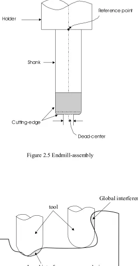
Figure 2.5 Endmill-assembly 9

Figure 2.6 Cutter interference 9

Figure 2.7 Rolling ball method for gouging detection 10 Figure 2.8 Discretized model for gouging detection 11 Figure 2.9 Inverse tool offset to construct gouge-free CL surface 12 Figure 2.10 Clean-up regions in a polyhedral model 13 Figure 2.11 Generate gouge-free tool paths by offsetting 13 Figure 2.12 The tool is fit into cavity by approaching the target point 14 Figure 2.13 Relationship between tool-path length and larger cutter diameter 15 Figure 2.14 Evaluate the maximal interpolation error by the sampling method 16 Figure 2.15 Subdivision method for curve interpolation 17 Figure 2.16 A typical stability lobe diagram for milling process 18 Figure 2.17 Analytic solution for chatter prediction for turning 19 Figure 3.1 The tool-path may not meet the machining tolerance requirement 24 Figure 3.2 Maximum error between a curve and a interpolating linear segment 25 Figure 3.3 Unit error vector H on a planar curve 30 Figure 3.4 Maximum errors within the interval 30 Figure 3.5 Chordal deviation for a planar offset curve 34 Figure 3.6 Relationship between interpolation error and machining error 36

Figure 3.7 Adaptive interpolation process 39

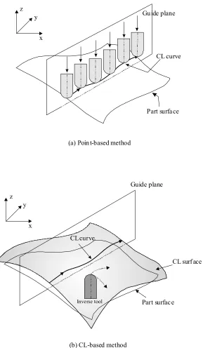
Figure 3.8 The secant method to find the root for adaptive interpolation 40 Figure 4.1 Point-based and CL-based tool path generation methods 44 Figure 4.2 CL-surfaces may not necessary be the constant offset of the part surface

Figure 4.3 Definition of inverse APT cutters 49 Figure 4.4 The cutting profile of an APT cutter 50 Figure 4.5 Cutting profiles of inversed endmills 54 Figure 4.6 Cutting profiles along an arc trajectory 56 Figure 4.7 Swept envelopes along an arc trajectory 58 Figure 4.8 Cutting profiles along a Bezier curve and along a line 59 Figure 4.9 Swept envelopes along a Bezier curve and along a line 60 Figure 4.10 Offset vector for a fillet-endmill cutters 61

Figure 4.11 Classification of GCL-surfaces 62

Figure 4.12 Generate GCL-surfaces for polyhedral models 64 Figure 4.13 Examples of GCL-surfaces for a pyramid model 68 Figure 4.14 Overall steps to generate CL data for STL models based on ICP method

69

Figure 4.15 Constructing tool-path from the initial CL-curves 71 Figure 5.1 Clean-up regions in a polyhedral model 74

Figure 5.2 Clean-up path topology 76

Figure 5.3 The proposed contraction tool method for clean-up tool-path generation

77

Figure 5.4 Clean-up band for an intermediate clean-up cutter 79 Figure 5.5 Determining the size of intermediate clean-up cutters 79 Figure 5.6 Gouging detection for a given cutter 82 Figure 5.7 Finding the Clean-up boundary points 84

Figure 5.8 Constructing clean-up tool-path 86

Figure 6.1 Dynamic milling model 94

Figure 6.2 Cutting force in milling 95

Figure 6.3 Circular approximation 97

Figure 6.4 Link-list surface model 100

Figure 6.5 Poincare plot examples 102

Figure 7.1 Example curves for interpolation 107

Figure 7.4 Offset curves for the example pocket part 110 Figure 7.5 Adaptive interpolation method applied in pocketing 111 Figure 7.6 A computer mouse model and its contours for roughing 113 Figure 7.7 The interpolation errors for one roughing tool-path 114 Figure 7.8 Interpolation CC curves for finishing 115 Figure 7.9 The simulation result for machining the computer mouse 116 Figure 7.10 An example for evaluating tool-path accuracy 117 Figure 7.11 Two testing part surfaces (STL models) 118

Figure 7.12 Computation time comparison 119

Figure 7.13 GCL-surfaces for different endmills 120

Figure 7.14 Results for shoe model 121

Figure 7.15 GCL-surface for the mouse model 123

Figure 7.16 Tool paths for machining the mouse model 123 Figure 7.17 Examples of tool-path generation for some artistic parts 124 Figure 7.18 An example computer mouse model and its CC-net 126

Figure 7.19 The clean-up tool-paths 127

Figure 7.20 Simulation results to machine the example mouse model 128

Figure 7.21 An example shoe polyhedral model 129

Figure 7.22 Clean-up tool-paths for the shoe model 130 Figure 7.23 Simulation results to machine the shoe model 131 Figure 7.24 Stability lobes at 100% immersion 133

Figure 7.25 Stability lobes at 50% immersion 134

Figure 7.26 Stability lobes at 25% immersion 135

Figure 7.27 Stability lobes at 10% immersion 135

LIST OF TABLES

Page

CHAPTER 1

INTRODUCTION

1.1 Motivation and Research Objectives

Modern products usually need to be machined at high-accuracy and high speed in order to improve machining quality and to shorten the production time. To accommodate more functions and show elegant shapes, the product geometries are becoming more complex and difficult for machining planning. Although the parametric surface models still play important roles in the modern product design, there is an increasing trend that polyhedral models are becoming more popular because of their topology simplicity and portability with platform-independence. However, the computational techniques of processing polyhedral models for machining are still inefficient and not robust enough to support the high performance machining of polyhedral models.

The objective of this paper is to investigate and develop computational techniques to improve the machining performance, especially the machining accuracy and efficiency for machining polyhedral models. This paper intends to improve the machining efficiency by considering the multiple-size tools utilization, the geometry of part surfaces and physical property of high speed machining processes. Several research issues are discussed in this paper for high performance machining of polyhedral models:

• High accuracy curve interpolation for high performance machining of complex surfaces. The objective is to develop computational geometric techniques to improve the tool-path accuracy for high performance NC machining of complex surfaces.

• Clean-up tool path generation for machining polyhedral models using multiple-sizes cutters. The objective is to develop techniques for using multi-tools in roughing, finishing and clean-up machining to shorten total machining time. • High speed machining chatter prediction for high performance machining. Both

geometric characteristics and physical properties of cutting are considered to predict chatter and improve cutting accuracy for high speed machining.

The improved performance includes the machining efficiency measured by the machining time, machining accuracy measured by the interpolation errors in tool-path generation, and maximal depth of cut measured by the chatter limit in high speed machining. The computational techniques and algorithms proposed in this paper are expected to shorten the total machining time and to improve the machining accuracy.

1.2 Thesis Organization

The remaining sections of the paper are organized as follows: In Chapter 2, the current technologies of gouging detection, optimal tool selection, smooth curve interpolation and chatter prediction are first reviewed.

In Chapter 3, the importance of smooth curve interpolation for high-accurate tool-path generation is introduced. An adaptive interpolation method is discussed for interpolation error analysis of both 3D spatial and 2D planar curves.

Chapter 4 presents the computational techniques for constructing Generalized CL (GCL) surfaces for different types of endmills. An inverse cutting profile method is presented for constructing GCL-surfaces for high performance machining of polyhedral models.

Chapter 6 presents the computational modeling of chatter prediction for high speed machining. By considering both the geometric and physical properties of cutting processes, a time-domain chatter prediction is proposed for high speed machining.

CHAPTER 2

LITERATURE REVIEW

Since the first numerical controlled (NC) machine was built in 1950s, various types of NC machines have been developed and commercialized. Among these different types of machines, milling machines are widely used in the die/mold industry and other industries to make complex products. This chapter briefly reviews the related state-of-art technologies for CAD/CAM/CNC, tool-path generation and chatter prediction in milling processes.

2.1 Geometric Models for Tool-path Generation

There are various approaches to represent a product model for the machining process. These different representations can be classified into three categories:

Figure 2.1 The wireframe model of a computer mouse

(1) Wireframe models

characteristic curves are the silhouette curves. However, wireframe models do not contain the surface information. They are not so popular for current CAM systems for NC tool-path generation.

(2) Surface models

Surface models represent shapes with a list of surfaces, where a surface denotes a two-dimensional submanifold of three-dimensional Euclidean space [Mathworld 02]. Surface models are widely used in the tool-path generation because machining processes usually deal with the outer shape of products. Among those different kinds of surfaces, two kinds of surface forms are widely used in tool-path generation:

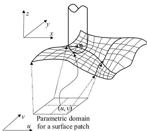
Figure 2.2 The parametric surface model of a computer mouse

• Parametric surface models

For every point on a parametric surface, each of its coordinates is represented separately as an explicit function of independent parameters. i.e.:

)) , ( ), , ( ), , ( ( ) ,

(u v x u v y u v z u v

S = (2.1)

where (u, v) are independent parameters defined in the parametric domain, S(u,v) is a

Among different types of parametric surfaces, the NURBS surface is an important type of parametric surface served as the exchange standard in CAD/CAM systems. A trimmed NURBS surface is defined by a set of ordered trimming loops along with the base NURBS surface. A NURBS surface is usually defined in the following form [Piegl 97]: ∑ ∑ ∑ ∑ = = = = = _n i m

j i j ip jq n

i m

j i j i j i p jq v N u N w v N u N P w v u S

0 0 , , ,

0 0 , , , ,

) ( ) ( ) ( ) ( ) , ( (2.2)

where P_i,j are the control points, w_i,j are the weights for corresponding control points,

and N_i,p and N_j,q are the degree p and q B-spline basis functions defined over the following knot vectors:

        = + − − +

+43 123

42 1 1 1 1 1 ,... , , ,..., , ,..., , p p r p p b b b u u a a a

U (2.3)

        = + − − +

+43 14243

42 1 1 1 1 1 ,... , , ,..., , ,..., , p p s p p d d d v v c c c

V (2.4)

where 1r=n+ p+ and s=m+q+1. Each trimming curve in the trimming loop can also

be represented in the NURBS form as [Piegl 97]:

(

)

∑

∑

   

    =

+ − − +

+43 14243

42 1

1 1 1

1

,... , , ,..., ,

,..., ,

p p t p p

f f f u u

e e e

U (2.6)

where 1t =n+ p+ . The trimming curves are properly connected to form outer and inner

trimming loops. Trimming loops are defined in the 2D parametric domain. The outer loops are oriented counter-clockwise, while inner loops are oriented clock-wise.

Figure 2.2 shows a typical parametric surface model of the mouse corresponding to the wireframe model in Figure 2.1. For the parametric surface shown in Figure 2.2, it has both concave and convex regions. The concave region may cause tool gouging if a large tool is used to machine this concave region. Gouging detection and tool selection are important topics and will be discussed in depth in this paper.

• Polyhedral surface model

Different from parametric surfaces, a polyhedral surface model usually consists of a collection of polygons. A polygon is a closed plane bounded with n-sides - usually linear segments. Among different types of polyhedral models, STL is one of the most popular representation formats. In STL models, each facet is a triangular polygon, and the normal information of each facet is also recorded.

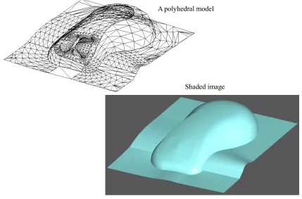
Figure 2.3 shows a polyhedral mouse model tessellated from the parametric surface shown in Figure 2.2. Compared with the shaded image in Figure 2.2, the shaded image of the polyhedral model in Figure 2.3 is rougher. If better accuracy of polyhedral models is required, more triangular facets are usually needed to represent the free-form surfaces. However, with the hardware and software advances of computer technologies, current computers can deal with large number of triangular facets without difficulty. The bottleneck now exists in finding better approaches to handle these polyhedral models for machining automation.

tool-path generation process because the related computation is much simpler for polygons (especially triangles) compared to the parametric surfaces. Machining of polyhedral models is becoming prevalent in recent years. This paper deals with the development of computational techniques for machining polyhedral models.

Figure 2.3 The polyhedral model of a computer mouse

A polyhedral model

Shaded image

(3) Solid models

In the following section, the gouging detection strategies for machining both parametric surfaces and polyhedral surfaces are discussed.

Figure 2.4 The solid model of a computer mouse

2.2 Gouging Detection and Optimal Tool Section

As shown in Figure 2.5, an endmill-assembly consists of four elements [Choi 98]: cutting edge, shank, holder and dead-center, where dead-center is the center region of the endmill-bottom which has no cutting capability. The actual cutting actions take place only at the cutting-edge. However, if any other tool element other than cutting-edge intrudes into the part surface, cutter interference occurs. In this paper, we mainly deal with two types of interferences: local interference and global interference. As shown in Fig 2.6, local interference is referred to the cutting-edge protrusion into the part surface. On the other hand, global interference is referred to the shank protrusion into the part surface. In this paper, the cutter interference with the dead-center and tool holder is not considered, and gouging is interchangeable with interference.

workpiece Local interference

Global interference tool

Figure 2.6 Cutter interference

Shank

Cutting-edge Holder

Refer ence point

Dead-center

2.2.1 Gouging detection for parametric surface models

Gouging detection for parametric surfaces can be classified as two major types:

) (u,v

S Part surface

Offset surface

a

P

b

P

o

P

Clean-up region

Figure 2.7 Rolling ball method for gouging detection

(1) Using surface model directly. This approach usually uses marching-based algorithm to trace the boundary of clean-up regions. Lee, et al., (2000) proposed a rolling-ball method for clean-up region identification. Its basic idea is similar to using a ball rolling around the surface concave regions. As shown in Figure 2.7, a ball with radius of r is used to find the boundaries of clean-up regions. Hence, the key step is to find the point couples (P_a,P_b) that has the same curvature center

o

P and P_oP_a = P_oP_b =r [Lee 00]. Similarly, Lo (2000) proposed the marching algorithm to find the interference boundary curve for two-stage tool-path scheduling.

u v

x y z

) , (u v

Parametric domain for a surface patch

n

Figure 2.8 Discretized model for gouging detection

• Curvature-based interference detection. When discrete points are sampled on a given surface, their curvature information is also computed [Yang 99]. The initial interference regions are identified by those points which have curvature

larger than

c

r

1 , where r_c is the cutter radius. Then complete interference is

checked around those interference regions,

• Coordinate-based interference detection. For a given surface and the discrete points sampled from it, the initial interference regions are identified by the actual coordinate and normal information of the discrete points. Then, complete interference is checked around those interference regions [Choi 89].

usually computational expensive [Choi 98]. However, with the advancing of computer hardware and software, the C-space method may have more applications.

Inverse tool CL-surf ace

Designed p art surfac e

Figure 2.9 Inverse tool offset to construct the gouge-free CL surface

2.2.2 Gouging detection for polyhedral surface models

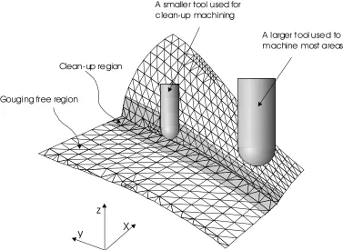
As shown in Figure 2.10, a polyhedral surface can be classified into two types of regions according to the machinability of a given cutter: gouge-free regions and clean-up regions. However, clean-up region identification is a non-trivial problem for polyhedral models. The difficulty stems from the fact that the original surface geometry information is lost and the sharp corners in polyhedral models may cause incorrect gouging detection at the concave region.

Conventionally, there are two ways to solve the problem. One approach requires offsetting the polyhedral model and linking the CL-curves [Jun 02]. As shown in Figure 2.11, this method generates gouge-free tool paths directly from the polyhedral models by offsetting. Then the pencil-cut paths are extracted from the calculated CL-paths. Another approach is briefly described as follows. As shown in Figure 2.12, to machine a target point P, the tool is dropped along Z-axis and is fitted into the cavity while approaching

and target point is calculated. If _dmin _{is less than a given tolerance, the target point P is}

treated as machinable and gouging free. Otherwise the target point P is treated as a gouging point.

Figure 2.10 Clean-up regions in a polyhedral model

X y

z Gougi ng free region

Clean-up region

A larger tool used to machine most areas A smaller tool used for

clean-up machining

polyhedral model Offset elements

Sharp-turn point

Figure 2.12 The tool is fit in the cavity by approaching the target point min

d

The 1st

touching point _{The 2nd}

touching point

r

y z

P

target point

Both of the above methods require generating gouge-free cutter location information, which is not a trivial problem especially for complex surface shapes.

2.2.3 Multiple tools applied in the machining process

The production cost of mechanical parts largely depends on the machining of the parts. Using multiple tools can greatly reduce the total machining cost, i.e., a larger tool is used to machine most of the surface area; while a smaller tool is used to remove the uncut material in the clean-up regions shown, as shown in Figure 2.10 [Lo 00]. When multiple tools are used, the larger the tool, the shorter the tool paths for the same surface finish and higher feed-rate can be applied. However, a large tool may leave large clean-up regions where a smaller cutter should be used to remove the uncut material. Figure 2.13 shows the total tool-path length related to the cutter selection strategy. In the figure, just two tools are used for finishing and clean-up machining. Since the smaller tool needs to finish the uncut area, usually its size can be decided by the maximal curvature information on the surface [Lo 00]. The tool-path length varies with different cutter sizes,

length L_opt can be achieved. The objective of tool selection is to find the optimal combination of tools to achieve the shortest total tool-path length and total machining time.

min

r ropt rmax

opt L

larger cutter diameter

Tool-path length Tool-path length _{for larger cutter} for smaller cutterTool-path length Total Tool-path length

Besides the machining time, the machining accuracy is also an important issue to be considered in tool-path generation. In the following section, different approaches to improve the tool-path accuracy are discussed.

2.3 Curve Interpolation in Tool-path Generation

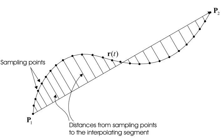
Sampling points

Distances from sampling points to the interpolating segment

Figure 2.14 Evaluate the maximal interpolation error by the sampling method 1

P

2

P

) (t

r

2.3.1 Sampling methods

One approach to evaluate the curve interpolation error is to estimate the maximal

error by sampling. Figure 2.14 illustrates the sampling method for an offset curve _ro(t)_. The chordal deviation is determined as the maximal distance from the sampling points to the interpolating segment P₁P₂ , as shown in Figure 2.14. If the estimated error is larger

2.3.2 Subdivision methods

The subdivision methods [Piegl 98, Piegl 99] are widely used for curve interpolation. They utilize the convex hull property of the polynomial splines such as

Bezier curves and B-spline curves. As shown in Figure 2.15, 0 0 V , 0

1 V , 0

2 V , 0

3

V are the

initial control points of a Bezier curve. The perpendicular distances are checked from the

inner control points 0 1

V and 0 2

V to the chord 0

3 0 0V

V . If any of the deviation distance is

larger than the acceptable interpolation tolerance, the curve is subdivided into two

sub-curves defined by 1 0 V , 1

1 V , 1

2 V , 1

3

V and 1 3 V , 1

4 V , 1

5 V , 1

6

V . For each subdivided curve,

distances are checked again from the inner control points to the chord, as shown in Figure 2.15. The iterations continue until the sub-curves satisfy the predefined interpolation tolerance. Generally, the subdivision method is stable and fast. However, since the offset curve of a planar polynomial curve is usually not a polynomial curve any more, the convex hull property for the offset curve is usually not valid. The traditional subdivision methods encounter difficulties to generate accurate interpolating point sequence for offset curves.

Figure 2.15 Subdivision method for curve interpolation

0 0 V

0 1

V 0

2 V

0 3 V

1 0 V

1 1 V

1 2 V

1 3

V V14

1 5 V

1 6 V

2.4 Chatter Prediction in High Speed Machining

High-speed machining (HSM) has received wide attention in both academic research and industrial applications in recent years. High speed machining can be defined as the tooth frequency ranging from 0.4 to 1.5 times the dominant natural frequency of the machine-tool system. Compared with traditional machining, high speed machining can achieve a much higher material removal rate. It can improve the production efficiency and surface finish with substantial cost savings. However, in high-speed machining, dynamic errors and machining stability become more apparent and difficult to control. Chatter prediction and control is an important prelude to the effective use of high speed machines.

3781.8 _{6441.1 9100.4 11759.7} 14419.1 _17078.4 19737.7

5 10 15

Figure 2.16 A typical stability lobe diagram for milling process lim

a

) , (s₁ a₁

) , (s₂ a₂

) , (s₃ a₃

unstable zone

Stable zone

2.16, at peak points like(s₁,a₁), (s₂,a₂) and (s₃,a₃), the axial depth of cut can achieve local maximum. If the machining spindle speed is chosen around those peak points, much higher axial depth of cut and material removal rate can be achieved without chatter. So it’s important to compute the stability lobes by chatter prediction in high-speed machining.

y c

y k

) (t T y

) (t y

f

0 h

h

) (t T y )

(t y

f F

f F

Figure 2.17 Analytic solution for chatter prediction for turning

flexible in the direction of feed, and the feed cutting force F_f causes the shaft to vibrate. The initial shaft surface does not have waves during the first revolution, but the tool starts to produce the wavy surface behind because of the bending vibrations of the shaft. When the second revolution starts, the surface has waves both on the cutting surface y(t) and

on the surface y(t−T) left by the previous cutting. Hence, the resulting dynamic chip

thickness is no longer constant but varies as a function of vibration frequency and the speed of the workpiece. The regenerative cutting forces may cause the tool vibration to be exaggerated to chatter. More details can be found in [Altintas 00].

The approaches to obtain chatter stability lobes can be classified as analytic and time-domain solutions. Different solutions will be discussed and compared in Chapter 5.

2.5 Summary

CHAPTER 3

MAXIMAL ERROR INTERPOLATION OF SMOOTH

POLYNOMIAL SPLINE CURVES FOR HIGH PERFORMANCE

MACHINING

This chapter presents an explicit solution approach to calculate the exact maximal interpolation errors for cubic free-form curves and the offset curves. To solve the maximal interpolation errors, the exact locations of the maximal error points are found by solving polynomial functions explicitly. Based on the explicit error formulation, an adaptive interpolation method is proposed to interpolate cubic free-form curves and their offset curves accurately. Compared with conventional approaches, the adaptive interpolation method ensures interpolation accuracy and generates fewer interpolation points for free-form curves and their offset curves. The proposed method can be used for high-accuracy curve interpolation and NC tool-path generation in CAD/CAM systems. Computer implementation and practical examples are also presented in this chapter.

3.1 Introduction

Modern products usually have complex shapes that need to be machined by CNC machines with highly accurate tool paths. However, current curve interpolation methods of using approximation may not always guarantee tool-path accuracy [Choi 99, Lee 97].

As shown in Figure 3.1, a cutter is used to machine a cutter contact (CC) curve r(t)

with a given tolerance τ . One of the traditional methods is to use circular arcs to

error ε_s ≤τ , the actual error is εo >τ_{, as shown in Figure 3.1. Therefore, the cutter will} cut into the part surface with the actual error ε0 _{larger than the given tolerance τ . In this}

case, the part may not be acceptable to meet the high accuracy requirement in manufacturing. The problem arises from the incorrect calculation of the interpolation error (also called the chordal deviation error). Traditionally, chordal deviation is estimated either by circular approximation or convex hull properties. In circular approximation approaches, chordal deviation is estimated based on the approximation arc around the interpolation points [Choi 99, Filip 86, Guenter 90, Yang 02]. The second approach is the subdivision method based on the convex hull property of free-from curves such as Bezier curves and B-spline curves [Anglada 99, Hilton 91, Piegl 99]. Despite its advantages of stability and efficiency, the subdivision method may encounter difficulties in interpolating offset curves, which are widely used in NC tool-path generation such as profiling and contour machining. The difficulties stem from the fact that the convex hull property may not be valid for the offset curves and it is hard to estimate their chordal deviations.

In high accuracy machining, it is important to ensure that the interpolation error is within a given tolerance [Koc 00, Lee 92]. In this chapter, explicit solutions are proposed to calculate the exact chordal deviations of cubic free-from curves and their offset curves. Instead of being approximated, the choral deviation can be calculated explicitly by solving polynomial functions [Ren 02b]. Based on the explicit chordal deviation solutions, an adaptive interpolation method is proposed to interpolate free-form curves and offset curves accurately [Ren 03]. In this chapter, the most common cubic free-form curves are used for formulation and illustration.

followed by the summary in Section 3.7.

i

P P_i+1

i O

) (t

r

Figure 3.1 The tool-path may not meet the machining tolerance requirement 1

+

i O

Circular approximation

τ

ε ≤_s ε >o τ

3.2 Maximum Error Conditions of Curve Interpolation

As shown in Figure 3.2, an interpolating linear segment P_iP_i+1 passes through

) ( ) ( )

(t r t Qt

h = − =[r(t)−Pi]−{[r(t)−Pi]⋅E}E (3.1)

where E is the unit chord vector defined as

i i i i P P P P E − − = + + 1

1 _{. To find the maximum}

interpolation error, let F(t) be the square of the error vector h(t) shown as follows:

2

) ( )

(t t

F =h = )h(t)⋅h(t (3.2)

By differentiating Equation (3.3.2), one can find the following:

) ( ) ( 2 ) ( t t dt t dF h h ⋅&

= (3.3)

From Equation (3.1), the first derivation of the error vector h(t) can be found as follows:

E E r r h

h( )= ( ) = (t)−{ (t)⋅ } dt

t d

t & &

& (3.4)

From Equations (3.3) and (3.4), one can find the following:

{

}

h ⋅ − ⋅ ⋅

= & & (3.5)

Figure 3.2 Maximum error between a curve and a interpolating linear segment ) (t r ) (t r_& ) (t Q ) (i

i r t

P =

) ( 1

1 +

+ = i

i r t

P ) (t h i t P r( )

E

and )h(t are perpendicular to each other, i.e., E⋅h(t)=0. Therefore, Equation (3.5) becomes

) ( ) ( 2 ) (

t t dt

t dF

r h ⋅&

= (3.6)

In Equation (3.6), the maximum of a curve interpolation error h(t)_max exists when

0 ) ( ₌ dt

t dF

. As shown in Figure 3.2, the maximum curve interpolation error h(t)_max

occurs if the following maximum chordal error conditions are satisfied:

0 ) ( )

(t ⋅h t =

r_& and h(t)≠0 (3.7)

Equation (3.7) means that the maximal curve interpolation error h(t)_max exists when

the tangential vector r&(t) and the error vector h(t) are perpendicular to each other, as shown in Figure 3.2. Equation (3.7) also shows that, without losing generality, the non-trivial solution exists when the error |h(t)| is not zero, i.e., h(t)≠0. Assuming that a

parameter _{t =t}* _{satisfies the maximum chordal error condition of Equation (3.7), the}

maximum curve interpolation error h(t*)max can be found by using Equation (3.1)

shown as follows:

2 *

* *

max

*_{) | [ ( ) ] [ ( ) ] {[ ( ) ] }}

(

|h t = r t −P_i ⋅ r t −P_i − r t −P_i ⋅E _(3.8)

The maximum error condition of Equation (3.7) and the maximum curve interpolation

error h(t)_max of Equation (3.8) can be used to interpolate free-from curves with a given accuracy, which will be discussed in the following sections.

function as follows: 3 3 2 1 0 2 )

(t a at a t a t

r = + + + (3.9)

where 3a_i,i=0,1,2, , are coefficient vectors. The coefficients a_i,i=0,1,2,3, can be calculated from the control points of Bezier curves and B-spline curves. Details of finding the coefficients a_i from the control points are presented in Appendices A and B. From Equation (3.9), the first derivative r_&(t) of the curve r(t) can be found as follows:

2 3 2

1 2 3

)

(t a a t a t

r& = + + (3.10)

As shown in Figure 3.2, r(t_i)r(t_i+1) is an interpolating linear segment of the curve r(t). The error vector h(t) was defined earlier in Equation (3.1). Substituting Equation (3.9) into Equation (3.1), one can find the error vector h(t) shown as follows:

E E r a a a a r a a a a

h( ) [ ( )] [( 3 ( )) ]

3 2 1 0 3 3 2 1

0 + + 2 + − − + + 2 + − ⋅

= t t t t_i t t t t_i

t

(3.11)

Rearranging Equation (3.11), one can get the following:

(

)

[

]

[

(

)

]

[

(

)

]

[

] [

]

E E a a E E a a E E a a h ) ) ( ( ) ( ) ( ) ( 0 0 1 1 2 2 2 3 3 3 ⋅ − − ⋅ − + ⋅ − + ⋅ − + ⋅ − = i i t t t t t t (3.12)

Since the interpolation linear segment passes through points r(t_i) and r(t_i+1) ,

0 ) ( )

(t_i =h t_i+1 =

h . h(t) can also be represented as follows:

) )(

)( ( )

( ₁ β₁ β₀

h t = t−t_i t−t_i+ t+ (3.13)

where β₁ and β₀ are coefficient vectors to be determined. By comparing Equation

(3.12) with Equation (3.13), we can find the coefficient vectors β₁ and β₀ shown as

(

)

β₁ = ₃ − ₃⋅ (3.14)

(

)

[

(

)

]

[

(

)

]

β₀ = t_i +t_{i+1 3}− ₃⋅ + ₂ − ₂ ⋅ (3.15)

Substituting Equation (3.13) into Equation (3.7), one can find the following equation:

(

)

) )(

(t−t_i t−t_i+1 β₁t+β₀ ⋅r& t = (3.16)

Equation (3.16) is a five-degree polynomial function and it has at most five roots. Among

the five roots of Equation (3.16), the two roots t=t_i and t=t_i+1 are known, i.e., h(t_i) =0

and h(t_i+1) =0. As shown in Figure 3.2, the maximal error h(t)_max doesn’t exist at

t=t_i and t=t_i+1 because the maximum error condition requires h(t)≠0 in Equation (3.7). Therefore, the remaining three unknown roots can be found by solving the following polynomial function from Equation (3.16):

(

)

Substituting )r_&(t of Equation (3.10) into Equation (3.17), a three-degree polynomial function is obtained as follows:

(

)

(

)

(

)

3 0 2 1 3 3

1⋅a + β ⋅a + β ⋅a + β ⋅a + β ⋅a +β ⋅a =

β t t t (3.18)

Equation (3.18) is a key function to find the maximum curve interpolation error h(t)_max . Detailed procedures of solving the remaining three roots are described in Appendix C. Using Equations (A20)-(A22) in the Appendix C, one can find the three remaining roots of Equation (3.18).

Based on Equation (3.13), a vector H(t)≡

(

)

(

)

[

(

)

]

[

(

)

]

( )

( ⋅E≡ β₁ +β₀ ⋅E

Since 0H(t)⋅E= in Equation (3.19), it indicates that H(t) is always perpendicular to

the chord vector E. As shown in Figure 3.3, when the curve r(t) is a planar curve,

) (t

h and H(t) are on the same plane where the curve is located. From Equation (3.13),

the error vector h(t) can be represented as follows:

Ω H

h(t)=(t−t_i)(t−t_i+1) (t)=(t−t_i)(t−t_i+1)ω(t) (3.20)

where ω(t) is the magnitude of an error vector H(t) and

E N

E N

Ω × ×

= is the unit error

vector perpendicular to the interpolating chord vector E; N is the normal vector of the plane on which the curve r(t) lies. In Equation (3.20), roots of (t−t_i)(t−t_i+1)ω(t)=0

cannot yield the maximal error; otherwise it would violate the condition h(t)≠0 as

discussed earlier in Equation (3.7). For planar curves, instead of solving Equation (3.18),

the parameter t of the maximal error h(t)_max can be found by substituting Equations (3.10) and (3.20) into Equation (3.7) shown as follows:

0 )

( 2 ) (

3 2 _{2 1}

3 + ⋅ + ⋅ =

⋅a Ω a Ω a

Ω t t (3.21)

Equation (3.21) is a two-degree polynomial function that can be solved easily.

As mentioned earlier, the feasible parameter solution t of Equations (3.18) and

(3.21) has to be within the parametric range of (ti, ti+1), i.e the parameter t should be

within the range of (t_i ≤t≤t_i+1), as shown in Figure 3.3. In some cases of complex curve

shapes, more than one feasible root can be found when solving Equation (3.18) or

Equation (3.21). The maximal chordal deviation h(t)_max is determined by selecting the

one that has the largest error h(t). For the example shown in Figure 3.4, three valid

roots * 1 t , *

2

t and *

3

t are found. ( *)

2 t

h is the largest among (*)

1 t

h , ( *)

2 t

h and ( *)

3 t h . Therefore, ( *)

2 t

h is assigned as the maximal chordal deviation h(t)_max for the linear

Figure 3.3 Unit error vector H on a planar curve )

(t_i

r

) (t_i+1

r

) (t

h

) (t

r N

E

H

X

y

z

Figure 3.4 Maximum errors within the interval )

( * 2 t

r

) (*

1 t

r ₍*₎

3 t

r

) (t_i

r r(ti+1)

) ( *

1

t

h

) ( *

2

t

h

) ( *

3

t

h

3.4 Finding the Chordal Deviation of Planar NURBS Curves

∑

∑

i i i

i i i i w t N w t N t V r (3.22)

where V_i are control points; w_i are the correspondent weights for the control points

i

V . )_N3(_t

i are B-spline basis functions discussed in the Appendix B. Define two

polynomial functions A(t) and B(t) shown as follows:

∑

3 ( )

) (

i

i i i t w N t

t t

t a a a a V

A (3.23)

∑

3 ( )

) (

i i i

w t N b t b t b t b t B (3.24)

where the coefficient vectors a_i,i=0,1,2,3, can be evaluated from Equations (A10)-(A13) in Appendix B; the coefficient b_i,i=0,1,2,3, can be evaluated by the similar

procedure for a_i except that the weights w_i are used instead of control points w_iV_i in Equation (3.23). Therefore, a NURBS curve r(t) can be represented as [Farin 99]:

) ( ) ( ) ( t B t t A

r = (3.25)

The first order derivative of r(t) is:

(

)

(

)

1 )

( ₂ B t t B t t

t B

t A A

r& = & − & (3.26)

According to Equation (3.7), the maximal chordal deviation h(t)_max occurs at:

(

)

(

)

) ( ) ( )

( ⋅ = ₂ ⋅ B t t −B t t =

t B

t t

t h h A A

r& & & (3.27)

0 )] ( ) ( )[ ( )] ( ) ( )[

(t t ⋅ t −B t t ⋅ t =

B A& h & A h (3.28)

Similar to the discussion of non-rational free-form curves in Section 3.3, for a planar NURBS curve, h(t) can be represented as follows (see Figure 3.3):

Ω

h(t)=ω(t) (3.29)

where ω(t) is the magnitude of an error vector h(t);

E N

E N

Ω × ×

= is the unit error

vector perpendicular to the interpolating chord vector E; N is the unit normal vector

of the plane on which the curve r(t) lies. Substituting h(t) into Equation (3.28) yields:

{

}

(t B t A& t ⋅Ω −B& t A t ⋅Ω =

ω (3.30)

The root of ω(t)=0 cannot be for the maximal error; otherwise h(t)=0 and the

condition of Equation (3.7) is violated. Therefore, Equation (3.30) can be simplified as follows:

0 ] ) ( )[ ( ] ) ( )[

(t A t ⋅Ω −B t A t ⋅Ω =

B & & (3.31)

From Equations (3.23) and (3.24), A&(t) and B&(t) can easily be derived as follows:

1 2 2

3 2

3 )

( a a a

A& t = t + t+ (3.32)

1 2 2

3 2

3 )

(t bt b t b

B& = + + (3.33)

Substituting )A(t , )B(t , )A&(t and B&(t) into Equation (3.31), the following equation can be obtained:

0

0 1 2 2 3 3 4

4t +c t +c t +ct+c =

c (3.34)

[

]

[

]

Equation (3.34) is a quartic polynomial function. It can be solved explicitly by the

method described in Appendix D. At most four roots of *

j

t , 4j≤ , can be found in

Equation (3.34). The maximal chordal deviation h(t)_max of a planar NURBS curve

occurs at the root * j

t that has the largest error ( *)

j t h .

For 3D spatial NURBS curves, the error vector h(t) no longer has the constant orientation as the error vector of a 2D planar curve does. The function to find the parameters for the maximal chordal deviation is usually higher than four-degree. According to Abel theory, the general polynomial equations of degree higher than four cannot be solved by purely algebraic methods [Pearson 74]. Some conservative estimation method using convex hull property can be used for estimating the chordal deviation of the 3D spatial NURBS curves [Piegl 98].

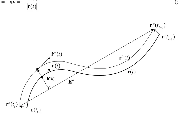
3.5 Finding the Maximum Chordal Deviation Error of Planar Offset Curves

In NC machining, offset curves are frequently used for profiling and contour machining. To ensure machining accuracy, it is important to calculate the chordal deviation of interpolating offset curves. Let v, m, and n be the tangential unit vector, the binormal unit vector and the principal normal unit vector of a parametric curve r(t), respectively. They can be defined as follows [Choi 91, Zhu 00]:

) ( ) ( ) ( ) ( t t t t r r r r m && & && & × ×

= (3.37)

[

]

[

]

= (3.38)

v m

n& =τ −κ (3.39)

where τ is the torsion and κ is the curvature of a point on the curve r(t).For a 2D planar curve, τ =0 and n& is simplified as follows:

) ( ) ( t t κ r r v n & &

& =−κ =− (3.40)

Figure 3.5 Chordal deviation for a planar offset curve )

(ti r

) (t_i+1

r o E ) (t o r_& ) (t h ) (t r ) (t o r ) (_i o _t r ) (_i+1

o _t r

) (t

r&

As shown in Figure 3.5, _ro(t) _{is the offset of a planar curve r(t). The offset curve} )

(t o

r can be defined as follows:

n r

) ( ) ( 1 ) ( t t lκ t o _r r r _& & & _

      −

= (3.42)

For an offset curve _ro(t)_{, Equation (3.42) indicates that the tangent vector r}o_(t)

& of an offset curve has the same direction with the tangent vector r&(t) of the original curve

) (t

r . As shown in Figure 3.5, ( ) o(_i+1)

i o _{t r t}

r is an interpolating linear segment of the

offset curve _ro(t)_{. E}o _{is the unit vector of ( ) ( )} 1 + i o i o _{t r t}

r and _ho(t) _{is the error vector}

from )_ro(t _{to ( ) ( )}

1 + i o i o _{t r t}

r , as shown in Figure 3.5. Since the error vector _ho(t) _is

perpendicular to the vector _Eo_{, one can find the following relationship:}

0 )

( ⋅ o =

o _{t E}

h (3.43)

According to Equation (3.7), the maximal error _ho(t)_{max of the offset curve r}o_(t)

exists if the following condition is satisfied:

0 ) ( )

(t ⋅ o t =

o _h

r& (3.44)

Substituting Equation (3.42) into Equation (3.44), the following equation can be obtained: 0 ) ( ) ( ) ) ( 1

( − t ⋅ t =

t

lκ _{r h}o

r_& & (3.45)

When a root _t* _{satisfies 0)}

) ( 1 ( * = − t lκ

r& and

(

*

* _{⋅ t ≠}

t _ho

r_&

)

& is

not perpendicular to _ho(_t*) _{and there must be a neighboring point that}

) ( )

(_t* o _t*

o _h

h ₊ > or _ho(_t*) _{> h}o(_t*)

− . Hence, t* cannot be the root parameter that

results in the maximal error and

) ( 1 _* t lκ r&

Rearranging Equation (3.45) yields the following relationship for finding the maximal

error _ho(t)_{max :}

0 ) ( )

(t ⋅_ho t =

r& (3.46)

Since )r(t and _ro(t) _{are planar curves, h}o_{(t) can be represented as follows:}

o o _{t t Ω}

h ( )=ψ( ) (3.47)

where ψ(t) is the magnitude of an error vector _ho(t)_,

o o o

E N

E N Ω

× ×

= is the unit error

vector perpendicular to the interpolating chord vector _Eo_{, and N is the unit normal}

vector of the plane on which the curve r(t) lies. In Equation (3.47), ψ(t) has non-zero value at the maximum error point. When the original curve r(t) is a non-rational

free-form curve, its first derivative was described earlier in Equation (3.10). To find the

maximal chord deviation _ho(t)_{max of the offset curve r}o_{(t), by substituting Equation}

(3.10) and Equation (3.47) into Equation (3.46), one can get the following relationship:

0 )

( 2 ) (

3 2 _{2 1}

3 + ⋅ + ⋅ =

⋅a Ω a Ω a

Ωo _t o _t o _(3.48)

Equation (3.48) has at most two roots and the one with larger error _ho(t) _{is selected as} the maximal error _ho(t)_{max of the offset curve r}o_(t).

When the original curve r(t) is a NURBS curve, its first order derivation has been described earlier in Equation (3.26). To find the maximal error parameter of the NURBS offset curve, the equation similar to Equation (3.34) can be deducted as follows:

0

0 1 2 2 3 3 4

4t +e t +e t +et+e =

[

]

[

]

o _(3.50)

Equations (3.49) and (3.50) are similar to Equations (3.34) and (3.35) except that Ω is

replaced by _Ωo_{. The procedures to solve Equation (3.49) are the same as those for}

Equation (3.34).

i

P P_i+1

i

O r(t)

1

+

i O

i

Q Q_i+1

j O j Q j P j G ) (t o h ) (t o r_& ) (t r&

Offset curve _ro(t)

Figure 3.6 Relationship between interpolation error and machining error

Inte rpolation error

Machining error

Equations (3.48) and (3.49) are very useful for evaluating the chordal deviation errors for the planar offset curves. Figure 3.6 shows the same example curve discussed

earlier in Figure 3.1. For the maximal error point O_j on the offset curve _ro(t)

& ,

Equations (3.44) and (3.46) indicate that the two tangents r&(t) and _r&o(t) _{are both} perpendicular to the error vector _ho(t)_{, as shown in Figure 3.6. Since the offset distance}

| |

|

|P_jO_j = Q_jG_j equals to the cutter radius, one can find that |G_jO_j |=|Q_jP_j | . Therefore, the interpolation error |G_jO_j | found by the proposed method is equal to the