Allocating Manpower with Absolute Partial Labor Flexibility to Optimize a Lower Bound on Lmax in Job Shop Scheduling Problems.

(1)

ABSTRACT

HAN, XIAOTIAN. Allocating Manpower with Absolute Partial Labor Flexibility to

Optimize a Lower Bound on Lmax in Job Shop Scheduling Problems. (Under the direction of Dr. Thom J. Hodgson.)

This research examines dual resource constrained job shop scheduling problems considering skill-limited labor as the second constraint, with the objective of minimizing maximum lateness. Absolute partial labor flexibility (APLF) is defined and modeled: a skill matrix is introduced to illustrate the skill structure of the workers in a job shop; and a worker allocation matrix is used to keep information on the number of workers in each worker group assigned to each machine group. The problem of determining whether a worker allocation is feasible under a given APLF situation is then formulated as an Allocation Feasibility

Determination (AFD) problem. Two existing LP based methods that can be used to solve the AFD problem are discussed. A new method that searches for worker reassignment from a feasible allocation to gain the allocation being tested (the PSP Method) is developed, where the worker reassignment is realized by a new search algorithm—the Path Searching

(2)

(3)

Allocating Manpower with Absolute Partial Labor Flexibility to Optimize a Lower Bound on Lmax in Job Shop Scheduling Problems

by Xiaotian Han

A thesis submitted to the Graduate Faculty of North Carolina State University

in partial fulfillment of the requirements for the degree of

Master of Science

Industrial Engineering

Raleigh, North Carolina 2012

APPROVED BY:

________________________________ ________________________________ Dr. Thom J. Hodgson Dr. Kristin A. Barletta

Committee Chair

(4)

ii

DEDICATION

(5)

iii BIOGRAPHY

Xiaotian Han was born in 1986 in Lanzhou, China. He started his undergraduate study in 2005 in Nanjing, China, which is 1500 miles away from his hometown, and received his Bachelor of Science in Applied Physics from Nanjing University in 2009. Xiaotian then relocated to Raleigh, North Carolina, which is 15000 miles away from his hometown, as an international graduate student in Department of Industrial and Systems Engineering in North Carolina State University.

(6)

iv

ACKNOWLEDGEMENTS

I would like to thank the following people:

 Zhengzhong Liu

 Dr. Thom Hodgson

 Dr. Kristin Thoney

 Dr. Russell King

 Dr. James Wilson

 Dr. Benjamin Lobo

 Zhuowei Wang

(7)

v

LIST OF TABLES

Table 1 Skill Matrix and the Associated Worker Allocation Matrix... 18

Table 2: Worker Allocation Matrix with Unknown Feasible Elements Values ... 20

Table 3 Polyhedron of the IP Formulation of Example 1 Represented in Matrix ... 21

Table 4 Cost Matrix of the Transportation Problem Associated with Example 1 ... 22

Table 5 Initial Worker Allocation Matrix for Example 1 ... 25

Table 6 Achieve Reassignment Request [1, 3] by the PSP – The Backward Path ... 29

Table 7 Achieve Reassignment Request [1, 3] by the PSP – Result Matrix ... 29

Table 8 Worker Allocation Matrix after Reassignment Request [4, 3] Achieved by the PSP ... 35

Table 9 Worker Allocation Matrix after Reassignment Request [4, 5] Achieved by the PSP ... 35

Table 10 Probability of a Job Being Routed through a Machine Group ... 45

Table 11 Statistics of the Running Times of the LBSA Using the Two AFD Methods ... 53

Table 12 (FM 0.8, irregular) Structure, S=5, T=5 ... 61

Table 15 Skill Matrix of the (FM 0.4, k-chain) Structure ... 62

Table 18 Skill Matrix of the (FM 0.4, irregular) Structure ... 63

Table 19 Skill Matrix of the (FM 0.3, irregular) Structure ... 64

(10)

viii

LIST OF FIGURES

Figure 1 Network Flow Model of Example 1 ... 20 Figure 2 Performance of Absolute Partial Labor Flexibility to Complete Labor Flexibility, Symmetric Job Shop, 80 Machines, 30% and 40% Staffing... 43 Figure 3 Performance of Absolute Partial Labor Flexibility to Complete Labor Flexibility, Symmetric Job Shop, 80 Machines, 50% and 60% Staffing... 43 Figure 4 Performance of Absolute Partial Labor Flexibility to Complete Labor Flexibility, Symmetric Job Shop, 80 Machines, 70% and 80% Staffing... 44 Figure 5 Performance of Absolute Partial Labor Flexibility to Complete Labor Flexibility, Symmetric Job Shop, 80 Machines, 90% Staffing, Micro-scaled ... 44 Figure 6 Performance of Absolute Partial Labor Flexibility to Complete Labor Flexibility,

Asymmetric Job Shop, 80 Machines, 30% and 40% Staffing ... 46 Figure 7 Performance of Absolute Partial Labor Flexibility to Complete Labor Flexibility,

(11)

1

Chapter 1

Introduction

Sequencing jobs in most job shop environments is an NP-Hard problem (Lenstra et al., 1977). During the past few decades, considerable effort has been spent on finding ways of getting optimal or near-optimal solutions (Mellor, 1966; Graham et al., 1979; Emmons, 1987; Baker and Scudder, 1990; Potts and Strusevich, 2009). The majority of this literature has dealt with scheduling in job shops constrained by machines only. There are several assumptions for this single resource constrained job shop (Lobo, 2011):

 Each job has a specific routing through the machines.

 There are no machine breakdowns.

 No preemption is allowed.

 Transportation time between different machines and set-up time on machines is

negligible (one can view the processing time of a job as already having the set-up time included).

 A machine can only process one job at a time, and a job can only be processed on one

machine at a time.

However, in the real world, a job shop is typically dual resource constrained or even multi-resource constrained. The number of workers available to operate the machines is often far less than the number of machines in the job shop (Gargeya and Deane, 1996).

(12)

2

the machines within it. The additional assumptions that transform the single resource constrained job shop into a dual resource constrained job shop are (Lobo, 2011):

 There are fewer workers than machines in the job shop.

 A machine group must have at least one worker assigned to it; otherwise it cannot

process any jobs.

 A machine takes one worker to operate it, and a worker cannot operate more than one

machine at a time.

 The allocation of workers, once determined, is static.

 Every worker can be assigned to any machine group in the job shop (complete labor

flexibility, CLF).

(13)

3

levels. The 100% level is “capable” while the 0% is “unable” in terms of the absolute

flexibility case. A new worker could have a 30% skill level while a veteran could have an 80% skill level.

The single resource constrained job shop scheduling problem with the objective of minimizing Lmax, denoted as N/M/Lmax, is NP-Hard. Hodgson et al. (1998) used a heuristic approach to solve this problem. Lobo (2011) added workers (labor) to the N/M/Lmax job shop scheduling problem. He developed a procedure to find the allocation of workers to machine groups in the job shop that optimizes a lower bound on Lmax, where the Virtual Factory, a heuristic scheduler developed by Hodgson et al. (1998) was used to generate a schedule for a given worker allocation. However, a feasible allocation under the complete flexibility

assumption may not be feasible in the partial labor flexibility situation.

In this thesis, a dual resource constrained job shop scheduling problem with absolute partial labor flexibility (APLF) is investigated. All the assumptions used in Lobo (2011), except for “every worker can be assigned to any machine group in the job shop” will be applied. The following additional assumptions regarding the partial flexibility issue will also be made:

 Each worker has a static skill pattern, i.e. this worker can only be assigned to a subset

of all the machine groups, which does not change over time.

 A certain worker (worker group) is either unable to operate machines in a machine

(14)

4

The minimization of Lmax is again used as the performance measure in this research, as it addresses the needs of on-time completion of jobs required by most companies (Ovacik and Uzsoy, 1996).

In this thesis, the APLF job shop scheduling problem is modeled, and the problem of determining whether a worker allocation is feasible in the APLF problem settings is defined as an Allocation Feasibility Determination (AFD) problem. A procedure that searches for feasible worker movement path and solves the AFD problem, the Path Searching Procedure (PSP), is developed. The Lower Bound Search Algorithm (LBSA) is extended to work in the APLF situation so that the optimal lower bound on Lmax can still be found. Then a series of

experiments are conducted to compare the optimal lower bounds obtained for the APLF job shop with the ones obtained for the CLF job shop.

In Chapter 2, a literature review and some background research are presented. In Chapter 3, new terms and definitions required by the AFD problem are introduced, the path searching procedure and two traditional methods that can be used to solve the AFD problem are

(15)

5

Chapter 2

Literature Review

In Section 2.1, literature on dual-resource constrained systems with partial labor flexibility is reviewed. The Virtual Factory approach to solving the N/M/Lmax problem is presented in

Section 2.2, and previous work on finding the allocation that optimizes the lower bound on

Lmax using complete labor flexibility is briefly described in Section 2.3.

2.1

Dual-Resource Constrained Systems with Partial Labor

Flexibility

Treleven and Elvers (1985) defined a dual constrained job shop as “one in which shop capacity may be constrained by machine and labor capacity or both. This situation exists in shops that have equipment that is not fully staffed and machine operators who are capable of operating more than one piece of equipment”. They also claimed that workers “may be transferred from one work center to another (subject to skills restrictions) as the demand dictates. When a work center is fully staffed, transfer of additional operators to that center will not increase capacity”.

Felan et al. (1993) studied how labor flexibility and staffing levels affect the

(16)

6

staffing level stands for each department having 7 workers assigned to it. They used mean flow time, average tardiness, and percentage of jobs tardy as performance measures, which “represent the primary drivers for measuring manufacturing performance in many

organizations” (Felan et al., 1993).

Their experiments showed that when the worker flexibility level increased given a fixed staffing level or the staffing level increased given a fixed worker flexibility level, the number of transfers increased, and the mean flow time, average tardiness and percentage of tardy jobs decreased. When the worker flexibility level and the staffing level both increased, all

incremental changes in the number of transfers, the mean flow time, average tardiness, and percentage of tardy jobs respectively diminished. Based on those results in the WIP and due-date performance, they concluded that a job shop (as they modeled it) with 60% staffing level and a medium worker flexibility level (level 2 or 3) is the optimal job shop.

“Although Felan et al. (1993) allow workers to transfer between departments, they are

concerned with finding the optimal staffing level and workforce flexibility level combination, rather than optimizing the allocation of workers to departments” (Lobo, 2011). Moreover, though partial labor flexibility was considered in their study, all workers are assumed to have the same level of flexibility once the worker flexibility level of the job shop is determined, which is a restricted case rather than a general case. There was no formulation of which departments each worker can be assigned to. Thus one cannot find the allocation of different workers among departments in the job shop.

(17)

7

flexibility. They claimed that “resource flexibility can have a significant impact on the quality of a schedule”, and “some resources are fundamentally flexible in that they are capable of migrating to processing centers as needed” (Daniels and Mazzola, 1994). “Labor

flexibility can be achieved by cross-training workers to develop the skills required to perform different tasks associated with multiple processing centers” (Daniels and Mazzola, 1994).

They termed the problem the flexible-resource flow shop scheduling (FRFS) and formulated it as a mixed integer program. They developed both optimal and heuristic methods to find the solution to the mixed integer program.

Daniels et al., (2004) did another study which extended their previous research on resource flexibility to a wider application—flow shop scheduling with absolute partial resource flexibility. In that paper, they defined resource flexibility as “the ability to

dynamically reallocate units of resource from one stage of a production process to another in response to shifting bottlenecks” (Daniels et al., 2004). They termed the problem the “flow shop rescheduling with partial resource flexibility problem” (FSPRF).

To formulate this partial flexibility problem, Daniels et al., (2004) introduced a very useful structure to keep the skill flexibility information of a flow shop—the skill matrix. Let

W be the set of all workers, and M be the set of all stations (machines). Also let w=|W| and

m=|M|. Then the worker-station skill matrix S is defined as a w×m matrix with element

{

(18)

8

introduced flexibility metric, FM, which simply computes the portion of “1” elements in the

skill matrix. Mathematically, it can be presented as

(∑∑ ) ⁄ . (2.1)

Other useful metrics defined by Daniels et al. (2004) are the station-balance metric and station worker-balance metric. The station-balance metric considers the difference between the station which has the largest number of workers capable to operate and the station which has the smallest number of capable workers. The station worker-balance metric splits the workers across stations which they can operate, based on the station-balance metric. A specially designed ideal skill matrix structure defined by Daniels et al. (2004) is the k -chain. It is an m×m matrix where type i worker can work k consecutive work stations, i

through i+k-1, where 0<k<m. For any i’>m, i’ [i,i+k-1], the corresponding work station i’ is made as work station i’-m. These chain structures satisfy the principles on the benefits of manufacturing process flexibility studied by Jordan and Graves (1995).

In the study of Jordan and Graves (1995), they considered how much flexibility is needed and how to configure flexibility for plants. The two principles they claimed were 1) “limited flexibility (i.e., each plant builds only a few products), configured in the right way,

yields most of the benefits of total flexibility (i.e., each plant builds all products)” and 2) “limited flexibility has the greatest benefits when configured to chain products and plants together to the greatest extent possible”, where a chain was defined to be “a group of

products and plants which are all connected, directly or indirectly, by product assignment decisions” (Jordan and Graves 1995). They went on to state that “within a chain, a path can

(19)

9

links”. Their experimental results illustrated that fewer (i.e. less links added) and longer (i.e.

more nodes connected) chains lead to more effective flexibility. This manufacturing flexibility configuration with plants and products is consistent with the worker skill flexibility configuration with workers (worker groups) and stations (machine groups). Therefore, the 2-chain structure as defined by Daniels et al., (2004) is the best single chain because it connects all workers (worker groups) and all stations (machine groups) with the fewest links.

Daniels et al., (2004) dynamically assigned absolutely partially flexible workers in a flow shop and studied the impact of that on the scheduling performance assuming that “the number of workers is equal to the number of work stations”. In that flow shop setting,

machines and workers are not grouped together, and the flow shop is fully stuffed. Thus, they did not need to consider a numerical allocation of workers among machine groups.

In summary, though there is a good deal of comprehensive research on both job shop and flow shop scheduling problems considering labor as well as the labor flexibility, based on our knowledge, there is no research on finding the optimal worker allocation in job shop scheduling with partial labor flexibility with the objective of minimizing Lmax. Most of the studies on partial labor flexibility focused on how different flexibility levels affect system performance, but none of them designed a detailed procedure of finding a numerical allocation of partially flexible workers in a job shop.

2.2

Virtual Factory solution for N/M/L

max

Problem

(20)

10

of the simulation is to determine the initial due date for each job i at each machine m. The latest possible time that a job can finish on machine m and still satisfy its final due date is termed slacki,m, and is computed as

∑ . (2.2)

Carroll (1965) found that slack did not perform well as a sequencing rule according to experiments, because queuing time is not considered when computing slack. Therefore, the Virtual Factory procedure incorporates queuing times into a revised slack measure to sequence jobs.

To estimate the queuing times, the Virtual Factory uses an approach proposed by

Vepsalainen and Morton (1988)—successive approximations using deterministic simulation. The job shop is first simulated using slacki,m as a sequencing rule. Queuing times are then

recorded for each job at each machine visited. Equipped with the queuing times (qij), a

“revised” slack can be calculated as

∑ ∑ (2.3)

where mi++ is the set of all operations after machine m on the routing machine list for job i

except the immediate subsequent operation. The simulation is run again using the revised slack from the previous iteration as the sequencing rule. This procedure will be repeated until the queuing times steady—usually 3 to 10 iterations—or the lower bound is achieved. The procedure can solve industrial scale problems in seconds.

To evaluate the quality of a schedule generated by the Virtual Factory for the N/M/Lmax

(21)

11

A well-known and useful method to calculate a lower bound was first developed by Carlier and Pinson (1984). Define the earliest possible start time for each job i on machine m as

∑ (2.4)

where mi- is the set of all operations previous to machine m on the routing machine list for

job i, and pij denotes the processing time of job i on machine j. Secondly, compute the latest

possible finish time for each job i on machine m as

∑ (2.5)

where di is the due date of job i, and mi+ is the set of all operations after machine m on the

routing machine list for job i. Then ESi,m can be treated as the effective release time (ri,m) for

job i on machine m. And similarly, LFi,m can be interpreted as the effective due date for job i

on machine m. Therefore, we can calculate the lower bound for every machine m, LBm, as a N/1/Lmax |ri,m problem. The lower bound for the N/M/Lmax problem, LB, is then

. (2.6)

This lower bound can be computed very quickly by the help of the relaxation suggested by Baker and Su (1974), which allows preemption of a job in process whenever a job with a more imminent due date becomes available. This lower bound is effective because there are

M opportunities to get a tight bound. This method was used as the method of obtaining a lower bound in the Virtual Factory.

(22)

12

the release time of jobs; Schultz et al. (2004) improved solution quality by incorporating simulated annealing; and Lobo (2011) transformed the Virtual Factory into a dual resource constrained job shop.

2.3

N/{M,W}

js

/L

max

Problem with Complete Labor Flexibility

2.3.1

Optimizing the Lower Bound on

L

max

In a dual resource constrained (DRC) system, how workers are allocated to each machine group may affect the performance of the job shop. As noted in Chapter One, Lobo (2011) developed a procedure to find the allocation of workers to machine groups in the job shop that optimizes a lower bound on Lmax. The problem was defined as a N/{M,W}js/Lmax job shop

scheduling problem. ∑ , where S represents the number of machine groups, and wi is

the number of workers assigned to each machine group. An allocation was denoted as

. The basic idea was to first compute the lower bound on Lmax for each

machine group and then find the maximum value over all machine groups. For a given allocation , the lower bound on Lmax for the job shop is

( ) . (2.7)

They defined the N/{M,W}mg/Lmax|rj,m job shop scheduling problem for each machine group.

The local release time and effective due-date for each job is determined using Equations (1.1) and (1.2).

Finding LBmg(Lmax) was formulated as a series of network flow problems, each testing to

(23)

13

Lobo (2011) added worker nodes to the network to effectively constrain the number of machines operated in each time period.

They used the out-of-kilter algorithm to determine whether the network flow formulation was feasible using a given trial Lmax value. A series of network flows were solved starting

with an Lmax value that allowed a feasible network, and decreasing the Lmax value by one unit until the network was infeasible. Since this network flow formulation allows for preemption, the smallest Lmax value that allows a feasible network is a lower bound on Lmax.

To find an initial feasible Lmax value for a machine group, a constructive algorithm was developed based on the method of solving the N/1/Lmax|rj,m problem with preemption that

considered worker availability. The main idea is that for each time t, the algorithm chooses the wi machines with the largest Lmax values to be operated so that the Lmax value of the

machine group can be minimized. Using the network flow model and the constructive algorithm, the lower bound on Lmax for any job shop with a given worker allocation can be

determined.

Lobo (2011) proved that “the lower bound on Lmax for a machine group is a discrete,

monotonic, non-increasing function of the number of workers assigned to the machine group”. He designed a search algorithm, named the Lower Bound Search Algorithm (LBSA)

to find an allocation that minimizes the lower bound on Lmax for the job shop. The algorithm starts with any given allocation . It first finds the set of constraining machine groups:

( ( )) . (2.8)

(24)

14

Algorithm 1 The Lower Bound Search Algorithm (LBSA) Set TC=2

Determine an initial allocation . 1.

Determine { ( ( ))}

Find { ( ( ))} If ( ) for any

TC=1 STOP. MINIMIZES ( ) FOR THE JOB SHOP. Else

Choose . Set

For If ( ) 2.

If

Find { ( ( ))} Choose

If ( ( )) ( ( ))

GO TO 2. Else

( ) ( ) ( ) ( ) If GO TO 2. Else

GO TO 1. Else

(25)

15

machine group”. Otherwise, one machine group is picked from K as the one the algorithm

needs to reassign an additional worker. The machine groups which cannot have worker unassigned from them for any reason are put into a set F. These reasons include: 1) the machine group is in set K; 2) the machine group has only one worker; 3) the machine group will have a lower bound on Lmax greater than the current lower bound after one worker is unassigned; 4) the allocation that is realized after unassigning one worker from the machine group is one of the allocations the algorithm has already tried. One machine group is picked from set J as the machine group the algorithm needs to unassign a worker from, where

( ( )) (2.9)

and F is initialized with the machine groups that satisfy the first and second reasons noted above. Finally, the machine groups in J that satisfied the third and fourth reasons noted above are put into set F; and one machine group that is proved to have worker to be unassigned is used to realize the reassignment with the objective machine group picked from K. After these four steps, an iteration is completed. The algorithm continues to search for improvement to the LB until termination CONDITION 2 is satisfied: “it is not possible to reassign a worker to the constraining machine group from any of the S-1 other machine groups”.

To conclude their study on the lower bound searching procedure, they proved that “the Lower Bound Search Algorithm (LBSA) is an optimal algorithm” (the LBSA will find an allocation with the minimum LB value).

2.3.2

Optimality Criteria and Performance Evaluation

(26)

16

optimality criteria which helps determine whether the allocation found by LBSA with the minimum lower bound—allocation is optimal. They defined the optimal allocation to be the allocation that allows the Virtual Factory to generate the schedule that has the minimum possible Lmax value for the N/{M,W}js/Lmax job shop. Second, they introduced a method for

evaluating the performance of an allocation by computing the probability distribution. Finally, they developed three heuristic searching strategies to find allocations which yield a smaller

(27)

17

Chapter 3

Optimizing the Lower Bound on

L

max

over Feasible Allocations

In Section 3.1, the Allocation Feasibility Determination (AFD) problem is defined and formulated, and notation and concepts useful in the discussion of this new problem are defined. In Section 3.2, two existing methods that can be used to solve the AFD problem are introduced. A new method named the Path Searching Procedure is developed and discussed in Section 3.3. In Section 3.4, the Lower Bound Search Algorithm (LBSA) is extended to the absolute partial labor flexibility (APLF) situation by using the Path Searching Procedure as the methodology to determine the feasibility of allocations.

3.1

New Problem Settings

As an extension to the study of Lobo (2011), this thesis will transform the Lower Bound Search Algorithm to find the allocation with the optimal lower bound for any given APLF situation. For each worker allocation proposed by the LBSA, we need to determine whether it is feasible in that APLF situation and to justify the answer. We first model this feasibility. There are some basic terms used in the following discussion:

 mgj – machine group j

 wgi – worker group i

 M – the set of all machine groups

 W – the set of all worker groups

 S = |M| – the number of machine groups

(28)

18

 ( ( ) ( ) ( )) – a given worker allocation

 ( ) – the number of workers in each worker group

3.1.1

Skill Matrix and Worker Allocation Matrix

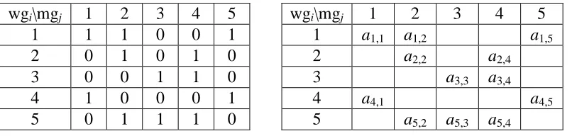
A skill matrix is an S by T matrix which is used to record the skillset information of each worker group, where each row represents a worker group and each column represents a machine group. The element of the matrix, si,j, equals 1 if the workers in worker group i are

trained to operate the machines in machine group j; it equals 0 otherwise. Note that the skill matrix is feasible if and only if there is no row or column whose elements are all zero

(Daniels et al., 2004). The combination of a skill matrix and the worker distribution vector, , uniquely defines a certain APLF situation.

The number of workers in each worker group that are allocated to each machine group is kept in the worker allocation matrix [A], where each element ai,j represents the number of

workers in worker group i that are assigned to machine group j. ai,j is defined as a feasible

element if the corresponding element si,jin the skill matrix equals 1, as infeasible elements

otherwise. ai,j’s can only have nonnegative integer values.

Table 1 Skill Matrix and the Associated Worker Allocation Matrix wgi\mgj 1 2 3 4 5 wgi\mgj 1 2 3 4 5

1 1 1 0 0 1 1 a1,1 a1,2 a1,5

2 0 1 0 1 0 2 a2,2 a2,4

3 0 0 1 1 0 3 a3,3 a3,4

4 1 0 0 0 1 4 a4,1 a4,5

(29)

19

We use an arbitrary APLF structure with 5 machine groups and 5 worker groups (S=5,

T=5) as an example. The skill matrix and the worker allocation matrix associated with it are shown in Table 1 above.

3.1.2

From Allocation to Allocation Matrix

A given worker allocation is feasible in a given APLF situation defined by a skill matrix and a worker distribution vector if and only if we can find nonnegative integer values for all feasible elements in the associated worker allocation matrix, so that the sums of the values of the feasible elements of each row in the matrix equal the numbers of workers in the

corresponding worker groups, and the sums of the values of the feasible elements of each column equal the numbers of workers assigned to the corresponding machine groups.

Specifically, given the skill matrix s and the vector of the number of workers in each worker group , we can claim a certain worker allocation as feasible if and only if we can find ai,j

for all ( ) {( ) }, such that

{

∑ ∑ ( )

(3.1)

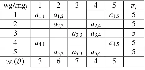
To better illustrate the allocation feasibility determination problem, we again use the skill structure in Table 1 as an example. We arbitrarily make = (5, 5, 5, 5, 5); and we design an arbitrary worker allocation = (3, 6, 7, 4, 5). The problem of determining feasibility of this worker allocation is then illustrated as Example 1.

(30)

20

Table 2: Worker Allocation Matrix with Unknown Feasible Elements Values wgi\mgj 1 2 3 4 5

1 a1,1 a1,2 a1,5 5

2 a2,2 a2,4 5

3 a3,3 a3,4 5

4 a4,1 a4,5 5

5 a5,2 a5,3 a5,4 5

( ) 3 6 7 4 5

We need to find a nonnegative integer solution for the following system of equations:

 a1,1+a1,2+a1,5=5; a2,2+a2,4=5; a3,3+a3,4=5; a4,1+a4,5=5; a5,2+a5,3+a5,4=5; a1,1+a4,1=3;

a1,2+a2,2+a5,2=6; a3,3+a5,3=7; a2,4+a3,4+a5,4=4; a1,5+a4,5=5. (3.2)

Figure 1 Network Flow Model of Example 1

An equivalent model is the network flow model depicted in Figure 1. In this network flow graph, the wgi nodes represent worker groups and the mgj nodes represent machine

(31)

21

groups. There is an arc from wgi to mgjif si,j=1. The arcs connecting the worker group nodes

and the source node must have a flow equal to the number of workers in each worker group. The arcs connecting the machine group nodes and the sink node must have a flow equal to the given worker allocation. Solving the AFD problem is equivalent to deciding whether a feasible flow for the network can be found.

3.2

Traditional Methods to Solve the AFD Problem

There are at least two traditional methods to solve the AFD problem: 1) formulate as a transportation problem with prohibited routes and homogeneous costs; 2) use the out-of-kilter method to determine a feasible flow.

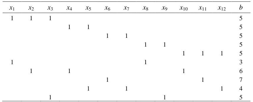
If we make the feasible elements (routes) as variables, make the feasibility condition (3.1) as constraints, we actually have defined a feasible region for an integer linear programming problem. The feasible region standard form polyhedron of the IP formulation of Example 1 is shown in Table 3.

Table 3 Polyhedron of the IP Formulation of Example 1 Represented in Matrix

x1 x2 x3 x4 x5 x6 x7 x8 x9 x10 x11 x12 b

1 1 1 5

1 1 5

1 1 1 5

1 1 3

1 1 1 6

1 1 7

1 1 1 4

(32)

22

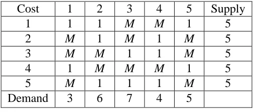
Because of the special structure of this IP model, which is actually a transportation problem with prohibited routes, we can use the transportation method to solve it. Make worker groups as suppliers, machine groups as customers, number of workers in each worker group as the supplies of each supplier, and the number of workers assigned to each machine group as demands of each customer. Each pair of worker group and machine group

connected by an arc has a route between them with consistent cost of 1; each of other pairs has a prohibited route between them with a cost of a big positive number M. Then the cost matrix can be written as in Table 4.

Table 4 Cost Matrix of the Transportation Problem Associated with Example 1 Cost 1 2 3 4 5 Supply

1 1 1 M M 1 5

2 M 1 M 1 M 5

3 M M 1 1 M 5

4 1 M M M 1 5

5 M 1 1 1 M 5

Demand 3 6 7 4 5

The corresponding transportation problem is to determine the shipping amount for each pair of supplier and customer so that the total cost is minimized. Any solution, with total cost smaller than M, yields a feasible flow for the network in Figure 1. This transportation

problem can be solved by the simplex method for transportation problems. For this particular problem, the transportation method took 6 iterations to find a solution.

(33)

23

and a set of node numbers that satisfy the kilter condition, by making change either in the circulation or in the node numbers. We apply Minty’s painting theorem to make the changes.

There are four steps of the method:

 Step 0: set the circulation to 0, set all node numbers to 0;

 Step 1: painting & labeling;

 Step 2: change in circulation, GO TO Step 1;

 Step 3: change in node numbers, GO TO Step 1.

Because there is no cost associated with each arc, cij=0 for all i, j, the change in node

numbers wi is calculated as

{ ( ) ( ) } (3.3)

where R is the set of red arcs and Y is the set of yellow arcs according to Minty’s painting theorem. This means the node numbers will never change after initialized as 0, in another word, the yellow-red cycle can be ignored. Therefore the out-of-kilter algorithm in this case consists of only the first three steps.

In addition to (3.3), we have

( ) (3.4)

where G is the set of green arcs. Therefore, the change in circulation, , is calculated as

{ ( ) }

(34)

24

where xij is arc number, lij is the lower bound, and uij is the upper bound of arc (i,j), sets with

“+” means arc numbers in those sets need to be increased and sets with “-” means arc

numbers in those sets need to be decreased (reverse arc direction).

The out-of-kilter algorithm found a feasible flow for the network of Example 1 using 8 iterations.

3.3

Worker Reassignment and Path Searching Procedure

In the following sections, we will introduce a more intuitive approach. Given a worker allocation matrix with arbitrary values on its feasible elements such that the feasibility condition for rows is satisfied, move workers within each row among machine groups until, the feasibility condition for columns, the desired worker allocation, is satisfied. Once the feasibility condition for rows is satisfied, how many workers of each type we have in the job shop and where different types of workers are located are illustrated clearly in a matrix form. Then the adjustment of the distribution of workers in each row can be interpreted more intuitively. This is one of the practical advantages of this method.

Without the constraints associated with the columns, the worker allocation matrix can be initialized easily. For instance, the worker allocation matrix for Example 1 can be initialized as shown in Table 5. From the table we can see that the current worker allocation is

(35)

25

Table 5 Initial Worker Allocation Matrix for Example 1

3.3.1

Definitions

Since the total number of workers is constant, the worker reassignments are realized in pairs, i.e. every time a machine group has a worker assigned to it, there must be another machine group that has a worker unassigned from it. We define a reassignment request as a pair of worker reassignments that need to be achieved together. Thus for each reassignment request, we define a source machine group (the source) as the machine group from which one worker needs to be unassigned, and an objective machine group (the objective) as the machine group to which one worker needs to be assigned. A reassignment request is represented as [p, q], where p is the index of the source machine group and q is the index of the objective machine group.

A reassignment request may be realized by one or more worker movements in series. The statement that one worker can be moved from machine group p to machine group q is equivalent to the one that machine group p has one worker to donate to machine group q. Workers can only be moved horizontally. In Table 5, for example, [1,5] can be realized simply by moving one worker in worker group 1 once, while [1,3] needs at least two steps

wgi\mgj 1 2 3 4 5

1 1 2 X X 2 5

2 X 3 X 2 X 5

3 X X 3 2 X 5

4 3 X X X 2 5

5 X 1 2 2 X 5

Current ( ) 4 6 5 6 4

(36)

26

(move one worker in worker group 1 from machine group 1 to machine group 2, then move one worker in worker group 5 from machine group 2 to machine group 3). We define a path for a given worker reassignment request as a set of ordered potential movements of workers in the worker allocation matrix that accomplish the request.

The search algorithm must be able to find a path for any reassignment request if one exists. Along with the source machine group and the objective machine group, we define a target machine group (the target) as an intermediary machine group from which a path is found to the objective machine group. The objective machine group is taken as the first target machine group.

3.3.2

Development of Path Searching Procedure

The basic idea of path searching is to start with the objective machine group and search backward for target machine groups until some target machine group, including the objective machine group, to which one worker can be moved from the source machine group is found. The algorithm should terminate either when a path for the original reassignment request is found or when all machine groups except the source are tested and no worker can be moved from the source to any of those machine groups. The algorithm can be briefly described as in the following four steps:

 Step 1: make the objective as the target and put it into the set of targets.

 Step 2: check if the source has a worker to donate to the target: if yes, done; otherwise,

(37)

27

 Step 3: search for a machine group that is not in the set of targets and has proper

worker to donate to the target: if found, set this machine group as the new target and put it into the set of targets, go to step 2; otherwise, go to step 4.

 Step 4: set the previous target as the target: if this machine groups is not the objective,

go to step 3; otherwise, the algorithm terminates in failure.

There are some set and variable definitions used in the Path Searching Procedure (PSP):

 Wgj – the set of indices of the worker groups that can operate mgj.

 Mgi – the set of indices of the machine groups that worker from wgi can operate.

 |Wgj| – the number of worker groups in Wgj.

 |Mgi| – the number of machine groups in Mgi.

 J – the set of indices of all target machine groups that are in the final path.

 K – the set of indices of all worker groups that the final path goes through

corresponding to the machine groups in J.

 U – the set of indices of the worker groups that the algorithm chose in Wgi’s

corresponding to all mgi’s in J.

 V – the set of indices of the machine groups that the algorithm chose in Mgi’s

corresponding to all wgi’s in K.

 G – the set of indices of target machine groups the algorithm has already found that

the source doesn’t have a worker to move to.

We present the PSP algorithm used for coding as Algorithm 2.

(38)

28

Algorithm 2 (PSP) Finding Path and Tracing Worker Movements for [p, q]. Part 1:

1. Set j=q, J1=q, m=1, n=1.

2. Set u=1, v=1.

Find out if mgp has worker of a worker group in Wgj.

If yes, say worker of wgk’ Wgj

Jn+1=p, Kn=k’. DONE, GO TO Part 2;

Else

Gm=j, GO TO 3.

3. Choose the uth worker group in Wgj, say wgk, search for the v

th

machine group in Mgk other

than mgj that has worker.

If found, say mgj’

If j’ is not in G

j=j’, Jn+1=j’, Kn=k, Un=u, Vn=v, m=m+1, n=n+1, GO TO 2;

Else if v<|Mgk|

v=v+1, GO TO 3; Else if u<|Wgj|

u=u+1, v=1, GO TO 3; Else if n>1

GO TO 4; Else

THE ALGORITHM FAILED TO ACCOMPLISH [p, q].

4. n=n-1, Jn+1=0, j=Jn, k=Kn.

If Vn<|Mgk|

v=Vn+1, u=Un, GO TO 3;

else if Un<|Wgj|

u=Un+1, v=1, GO TO 3;

else if n>1 GO TO 4; else

THE ALGORITHM FAILED TO ACCOMPLISH [p, q].

Part 2:

For i=1 to n

j1=Ji+1, j2= Ji, k=Ki,

(39)

29

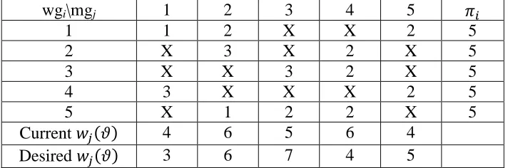
reassignment requests that potentially achieve the desired worker allocation are [1, 3], [4, 3], [4, 5], etc. We only discuss [1, 3] because the PSP works similarly on any other reassignment requests. The step-by-step process that the PSP uses to realize a worker reassignment request [1, 3] is described as follows and illustrated in Table 6 and Table 7.

Table 6 Achieve Reassignment Request [1, 3] by the PSP – The Backward Path

Table 7 Achieve Reassignment Request [1, 3] by the PSP – Result Matrix

p=1, q=3. Part 1:

1. Set j=J1=q=3. m=1, n=1.

2. Set u=1, v=1. Wgj={3, 5}. mgp does not have a worker in wg3 or wg5. Gm=j.

wgi\mgj 1 2 3 4 5

1 1 2 X X 2 5

2 X 3 X 2 X 5

3 X X 3 2 X 5

4 3 X X X 2 5

5 X 1 2 2 X 5

( ) 4 6 5 6 4

wgi\mgj 1 2 3 4 5

1 0 3 X X 2 5

2 X 2 X 3 X 5

3 X X 4 1 X 5

4 3 X X X 2 5

5 X 1 2 2 X 5

(40)

30

3. The uth worker group in Wgj is wg3. k=3. Mgk={3, 4}. The vth machine group in Mgk

other than mgj that has worker is mg4, j’=4. 4 is not in set G, so j= j’=4, Jn+1= j’, Kn=k, Un=u, Vn=v, m=m+1=2, n=n+1=2.

4. Set u=1, v=1. Wgj={2, 3, 5}. mgp does not have a worker in wg2, wg3 or wg5. Gm=j.

5. The uth worker group in Wgj is wg2. k=2. Mgk={2, 4}. The vth machine group in Mgk

other than mgj that has worker is mg2, j’=2. 2 is not in set G, so j= j’=2, Jn+1= j’, Kn=k, Un=u, Vn=v, m=m+1=3, n=n+1=3.

6. Set u=1, v=1. Wgj={1, 2, 5}. mgp has a worker in wg1, k’=1. Jn+1=p, Kn= k’.

Part 2:

a3,4=a3,4-1=1, a3,3=a3,3+1=4; a2,2=a2,2-1=2, a2,4=a2,4+1=3; a1,1=a1,1-1=0, a1,2=a1,2+1=3.

3.3.3

Properties of the Path Searching Procedure

Proposition 1: Given that at least one path exists for a given reassignment request, it is impossible that Algorithm 2 terminates in failure.

Proof. The Path Searching Procedure actually consists of a series of sub-problems. Every time the Algorithm sets a machine group as target, it starts to look at a new sub-problem. Assume the reassignment request is [p, q]. When the algorithm makes machine group j as the target, it is actually dealing with [p, j] with a worker allocation matrix excluding machine groups in set G.

Define Sub(n) as a formal sub-problem which represents any sub-problems with n

(41)

31

 Searching DONE, if the source has proper worker to donate to the target

 Sub(n-1), if a machine group other than the source that is not in G has proper worker

to donate to the target, the target will be put into G

 Sub(n), if none of the machine groups that are not in G has proper worker to donate to

the target, the previous target will be set as target

Then we use mathematical induction to prove Proposition 1 is true. Step 1: Start from n=1, Sub(1).

When there is only one machine group not in G and the algorithm did not finish in success, all machine groups except the source and the current target have been made as target at least once before, and the source does not have proper worker to donate to any of those targets. On the other hand, a path from the current target to the objective has been found. And this last “unvisited” machine group must be the source. If there is a path for this reassignment request, the source must have proper worker to donate to at least one of the other machine groups. In summary, the source must have a worker to donate to the current target. This means the algorithm successfully find a path for the request. The above analysis proves the base: Proposition 1 is true for n=1.

Step 2: Assume Proposition 1 is true when n=k. When there are k machine groups not in

G, if there is a path, Algorithm 2 will find one. PSP at Sub(k) will always find a path if one exists.

Step 3: Prove that Proposition 1 is still true when n=k+1, Sub(k+1).

(42)

32

only need to show that in the third case, Sub(k+1) finally will still result in Sub(k) if there is a path.

In the third case, the source does not have proper worker to donate to any of the m-k-1 machine groups including the current target and the objective in G. None of the machine groups not in G have a proper worker to donate to the current target. Then Sub(k+1) stays as Sub(k+1) with the previous target. If there is a path, there must be at least one machine group not in G that has a proper worker to donate to some of the machine groups in G. After several steps, the PSP at Sub(k+1) with some previous target will find the machine group not in G

that has a proper worker to donate to the target because the PSP searches every machine group not in G if needed. And this machine group not in G, once found, can be made as a new target because a path has been found from any machine group in G to the objective. Then Sub(k+1) changes to Sub(k). So we proved that if a path exists, Sub(k+1) will either finish in success, or result in Sub(k).

All in all, we proved that Proposition 1 is always true for any n=1 to S.

(43)

33

Lemma: If the PSP can achieve [pn+1, qn+1] when Path A was selected for [pn, qn], it can still

achieve [pn+1, qn+1] when Path B was selected for [pn, qn]; and vice versa.

In the statement, [pk, qk] represents the reassignment request for iteration k, and Path A and

Path B are two different possible paths in iteration n.

Proof. Before iteration n, Path A and Path B both exist for [pn, qn]. If the PSP can achieve

[pn+1, qn+1] after Path A was selected in iteration n, i.e. there is a path for [pn+1, qn+1] in

iteration n+1, after reassignment [pn+1, qn+1] in iteration n+1, the resulted allocation is proved

to be feasible. When Path B was selected in iteration n, the reassignment request is still [pn+1, qn+1] in iteration n+1, and we know that the allocation after this reassignment is feasible.

Therefore, the PSP can still find a path for [pn+1, qn+1].

If the PSP cannot achieve [pn+1, qn+1] after Path A was selected in iteration n, the

allocation after reassignment [pn+1, qn+1] will be infeasible. Therefore, even if Path B was

selected in iteration n, the PSP will still work on a request that leads to an infeasible allocation, which will terminate in failure.

Proposition 2: If the PSP can achieve [pn+k, qn+k] when Path A was selected for [pn, qn], it

can also achieve [pn+k, qn+k] when Path B was selected for [pn, qn] (k=1, 2 …); and vice versa.

Proof. If each one of the requests [pn+1, qn+1], [pn+2, qn+2], [pn+3, qn+3], …, [pn+k, qn+k] can be

achieved by the PSP in order when Path A was selected for [pn, qn]. According to the Lemma,

if Path B was selected, the PSP can also achieve [pn+1, qn+1]. After each iteration, since the

(44)

34

If the PSP cannot achieve [pn+k, qn+k] when Path A was selected for [pn, qn], without loss

of generality, we assume [pn+k, qn+k] is the first reassignment request after [pn, qn] that is not

achievable. Then we know that the allocation after reassignment [pn+k, qn+k] is infeasible.

Therefore, no matter which path was selected in iteration n, the PSP cannot achieve [pn+k, qn+k]

by any means.

Proposition 2 guarantees that when the PSP works on any given reassignment request in any given iteration, whichever path is used will not affect the achievability of any other reassignment request in the future iterations. This important property supports the methodology that the algorithm will stop once it finds a path and achieve the request.

3.3.4

Solve the AFD Problem with the PSP

Continuing the discussion at the beginning of Section 3.3, the method developed to solve an AFD problem can be summarized as follows. For any allocation feasibility determination problem, after the worker allocation matrix is initialized, there may be a difference between the worker allocation associated with the initial worker allocation matrix and the worker allocation being tested. Reassignment requests that may eliminate the difference are arbitrarily decided. Then the PSP is used to justify and achieve those requests; one request per iteration. If some of the requests cannot be achieved, the PSP will continue to try other possible requests until the difference is eliminated or no other reassignment request that could contribute to the elimination can be achieved. If the difference is finally eliminated, the worker allocation being examined is proved to be feasible in the corresponding APLF

(45)

35

Given the initial worker allocation matrix in Table 5, we can solve the AFD problem for allocation (3, 6, 7, 4, 5) by 3 iterations of the PSP. We arbitrarily make [1, 3], [4, 3], [4, 5] as the reassignment requests for each iteration respectively. We already have the worker

allocation matrix after [1, 3] achieved shown in Table 7. Now we present the matrix after the second and the third iteration as in Table 8 and Table 9.

Notably, the PSP Method took only 3 iterations to solve Example 1, which is less than the transportation method (6), and the out-of-kilter algorithm (8).

Table 8 Worker Allocation Matrix after Reassignment Request [4, 3] Achieved by the PSP

Table 9 Worker Allocation Matrix after Reassignment Request [4, 5] Achieved by the PSP

wgi\mgj 1 2 3 4 5

1 0 3 X X 2 5

2 X 2 X 3 X 5

3 X X 5 0 X 5

4 3 X X X 2 5

5 X 1 2 2 X 5

( ) 3 6 7 5 4

wgi\mgj 1 2 3 4 5

1 0 2 X X 3 5

2 X 3 X 2 X 5

3 X X 5 0 X 5

4 3 X X X 2 5

5 X 1 2 2 X 5

(46)

36

3.4

The Lower Bound Search Algorithm in an APLF situation

The reason for us to introduce and develop the allocation feasibility determination methods, as discussed at the beginning of this Chapter, is that we want to make the LBSA work in the APLF situation. The PSP Method and the out-of-kilter algorithm have an obvious advantage over the transportation method when embedded into the LBSA. In the LBSA, the only one worker allocation that needs to be tested as a complete AFD problem is the initial allocation

. And this AFD problem only needs to be solved once. Most of the time, the LBSA is trying to reassign one worker from one machine group to another machine group based on a known feasible allocation. The PSP and the out-of-kilter algorithm could directly test the feasibility of the reassignment and realize it in a single iteration, while the transportation method will have to solve complete problems. This is because the worker allocation matrix (the network flow) will be updated after each iteration of the PSP (the out-of-kilter

algorithm), thus every time the LBSA proposes a worker reassignment, the PSP (the out-of-kilter algorithm) only needs to run one iteration based on the worker allocation matrix (the network flow) obtained after the previous reassignment to decide if the reassignment request (the new flow) is achievable (feasible). In this research, the PSP Method is used as the allocation feasibility determination method for the LBSA. An experiment that compared the running times of the PSP Method and the out-of-kilter algorithm is discussed in Chapter 4, Section 4.4.

(47)

37

Algorithm 3 The Lower Bound Search Algorithm in Absolute Partial Labor Flexibility Situation Using the Path Searching Procedure to Determine Allocation Feasibility. Set TC=2

Determine an initial allocation . Solve AFD( ). Update . 1.

Determine { ( ( ))}

Find { ( ( ))} If ( ) for any

TC=1 STOP. MINIMIZES ( ) FOR THE JOB SHOP. Else

Choose . Set

For If ( ) 2.

If

Find { ( ( ))} Choose

If ( ( )) ( ( )) , GO TO 2.

Else

( ) ( ) ( ) ( ) If , GO TO 2. Else

If PSP(j,k) succeeds /*using the Path Searching Procedure to realize [j, k] , GO TO 1.

Else

, GO TO 2. Else

(48)

38

If this allocation is infeasible, according to the discussion in Section 3.3.4, the PSP Method must terminate at an allocation that is closest to the initial allocation. We name this allocation as the alternative initial allocation. Because of the optimality of the LBSA, we can use the alternative initial allocation to start Algorithm 3. As in the LBSA, if any one of the

constraining machine groups is already fully staffed, the termination CONDITION 1 will be satisfied. In Part 2 of Algorithm 3, the PSP is used to check if the proposed worker

reassignment request [j, k] is achievable. If a request is achieved, the allocation will be updated and Algorithm 3 moves on to the next iteration. If a request cannot be achieved, the source j will be put into the set of failure; and Algorithm 3 searches for other reassignments. As in the original LBSA, when all machine groups other than the constraining machine group are in the failure set, termination CONDITION 2 will be satisfied.

Proposition 3: Algorithm 3 finds a feasible allocation that satisfies for all feasible allocation .

Proof. We can prove Proposition 3 by extending the proof conducted by Lobo (2011) on the proposition that “the Lower Bound Search Algorithm finds an allocation that satisfies

for all allocation ”. Algorithm 3 terminates in allocation only if termination

CONDITION 1 or CONDITION 2 is satisfied. If Algorithm 3 terminated because

(49)

39

a) There is only one worker assigned to machine group j;

b) The lower bound on Lmax of machine group j after one worker unassigned from it is

larger than the current lower bound on Lmax of machine group k; c) Machine group j is a constraining machine group itself;

d) Reassignment request [j, k] cannot be achieved by the PSP.

Lobo (2011) already proved that it is impossible to find an allocation Ω that yields a smaller lower bound if any [j, k] satisfied condition a), b), and c). If the only machine groups that do not satisfy condition a), b), or c) satisfy condition d), a feasible allocation Ω that

yields a smaller lower bound still cannot exist, because all allocations that yield smaller lower bounds, the allocations after those reassignments, are proved to be infeasible in the given APLF situation. Therefore, allocation yields the smallest lower bound on Lmax in all feasible allocations.

(50)

40

Chapter 4

Computational Experiment

4.1

Experimental Design

Algorithm 2 and Algorithm 3 are coded in C++ and embedded in the Virtual Factory. The goal of this experiment is to test the difference in the lower bound on Lmax achievable when

there is not complete flexibility. Because this experiment is an extension of the experiment of testing the performance of the lower bound by Lobo (2011), the experimental job shop is the same with some additions. There are 80 machines and 10 machine groups in the job shop, where each machine group has 8 machines. The total number of jobs processed is 1200. Two different job shop types (symmetric and asymmetric) are used. Eight different due date ranges are tested: from 200 to 3000, with an increment of 400. Seven different staffing levels are applied: 30% (24), 40% (32), 50% (40), 60% (48), 70% (56), 80% (64), and 90% (72). All processing times are discrete random variables ranged from 1 to 40 with a uniform distribution. The number of operations of each job ranging from 6 to10, and at most 3 operations are in one machine group.

(51)

41

generated following two patterns. One pattern is the k-chain structure, i.e. k equals 3 when

FM equals 0.3 in this case. The other pattern is the “irregular” structure which is arbitrarily designed for comparison test. The irregular structure is defined as any skill structure that is not following a known pattern and is close to a random 1/0 matrix. In the real world, different job shops could have different irregular skill structures depending on how the job shop is configured and what types of workers are involved in the job shop. However, our experiment cannot cover all the possibilities though the methodologies developed in the previous chapters are capable of solving the problem with all possible skill structures. To generate a set of irregular structures in a relatively consistent way, we can set all elements of the skill matrix to “1”s first and then change some of the “1”s to “0”s in some structured way.

The procedure that is used in this experiment to generate the irregular structure is illustrated in Appendix A. Both two types of skill matrix will be tested and compared to the job shop performance with complete labor flexibility. Therefore, in total, we will test 6 absolute partial labor flexibility (APLF) skill structures and the complete labor flexibility (CLF) structure. All skill matrices used in the experiment are presented in the Appendix B.

According to the type of job shop and due-date range, randomly generated problems are defined. For each problem type with each staffing level, each FM value, and each type of skill structure, 50 randomly generated problems are solved.

4.2

Experimental Results

(52)

42

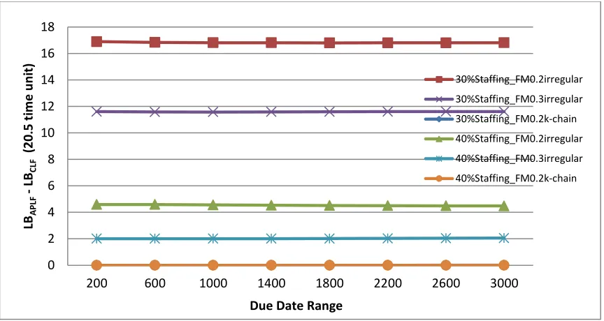
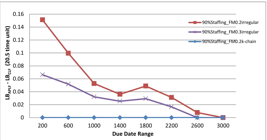
CLF situation (LBCLF) in each due-date range at each staffing level. Each line is a plot of

LBAPLF - LBCLF as a function of the due-date range and represents a specific skill structure as

noted in the legend. This value is used to represent the performance of the job shop with a particular combination of job shop type, due-date range, staffing level, FM value, and skill structure type. The closer the value is to zero, the better the performance of the job shop is in the certain APLF situation. For each job shop type and each staffing level, only three skill structures, (FM 0.2, irregular), (FM 0.3, irregular), and (FM 0.2, k-chain), possibly have nonzero LBAPLF - LBCLF. In other words, for all other skill structures, the lower bounds found

are always equal to the ones found in CLF situation. Therefore, we only present the

performance of these three skill structures in the first two sets of graphs in sections 4.2.1 and 4.2.2. The third set of graphs in Section 4.2.3 look at how the average performance varies by skill structure, where the performance is averaged by the due-date ranges and plotted for each staffing level. All performances are presented in units of the average processing time (20.5).

4.2.1

Performance vs. Due-date Range: Symmetric Job Shop

In the symmetric job shop, each machine group sees, on average, 10% of the work load that passes through the job shop. The graphs illustrating symmetric job shop performances are shown in Figure 2 to Figure 9. Based on these graphs, we can make the following

observations.

Generally, the performance is getting better when the staffing level increases, i.e. the higher the staffing level is, the smaller the average value of LBAPLF-LBCLF is for each skill

structure. However, close scrutiny shows that this positive correlation between the

(53)

43

Figure 2 Performance of Absolute Partial Labor Flexibility to Complete Labor Flexibility, Symmetric Job Shop, 80 Machines, 30% and 40% Staffing

0 2 4 6 8 10 12 14 16 18

200 600 1000 1400 1800 2200 2600 3000

LB AP LF LB CLF (20.5 t im e u n it) _{30%Staffing_FM0.2irregular} 30%Staffing_FM0.3irregular 30%Staffing_FM0.2k-chain 40%Staffing_FM0.2irregular 40%Staffing_FM0.3irregular 40%Staffing_FM0.2k-chain

Due Date Range

0 2 4 6 8 10 12 14 16 18

200 600 1000 1400 1800 2200 2600 3000

LB AP LF LB CLF (20.5 t im e u n it) 50%Staffing_FM0.2irregular 50%Staffing_FM0.3irregular 50%Staffing_FM0.2k-chain 60%Staffing_FM0.2irregular 60%Staffing_FM0.3irregular 60%Staffing_FM0.2k-chain

(54)

44

Figure 5 Performance of Absolute Partial Labor Flexibility to Complete Labor Flexibility, Symmetric Job Shop, 80 Machines, 90% Staffing, Micro-scaled

0 2 4 6 8 10 12 14 16 18

200 600 1000 1400 1800 2200 2600 3000

LB AP LF LB CLF (20.5 t im e u n it) 70%Staffing_FM0.2irregular 70%Staffing_FM0.3irregular 70%Staffing_FM0.2k-chain 80%Staffing_FM0.2irregular 80%Staffing_FM0.3irregular 80%Staffing_FM0.2k-chain

Due Date Range

0 0.02 0.04 0.06 0.08 0.1 0.12 0.14 0.16

200 600 1000 1400 1800 2200 2600 3000

LB AP LF LB CLF (20.5 t im e u n it) 90%Staffing_FM0.2irregular 90%Staffing_FM0.3irregular 90%Staffing_FM0.2k-chain

(55)

45

staffing level, the average value of LBAPLF - LBCLF decreases as the staffing level increases.

At the 50% staffing level, all average difference values equal to zero. But start from the 60% staffing level, the average value of LBAPLF - LBCLF for the (FM 0.2, irregular) structure

jumped to a value higher than the one with the same structure at the 40% staffing level; and the average value of LBAPLF - LBCLF for the (FM 0.3, irregular) structure jumped at the 70%

staffing level. At the 80% staffing level, the values of the two structures jumped again. At all but 80% staffing level, for each skill structure, LBAPLF - LBCLF is almost stable as the

due-date range changes. At the 8