Ensemble-Based Medical Relation Classification
Jennifer D’Souza and Vincent Ng Human Language Technology Research Institute
University of Texas at Dallas Richardson, TX 75083-0688
{jld082000,vince}@hlt.utdallas.edu
Abstract
Despite the successes of distant supervision approaches to relation extraction in the news do-main, the lack of a comprehensive ontology of medical relations makes it difficult to apply such approaches to relation classification in the medical domain. In light of this difficulty, we propose an ensemble approach to this task where we exploit human-supplied knowledge to guide the de-sign of members of the ensemble. Results on the 2010 i2b2/VA Challenge corpus show that our ensemble approach yields a 19.8% relative error reduction over a state-of-the-art baseline. 1 Introduction
Medical relation (MR) classification, an information extraction task in the clinical domain that was re-cently defined in the 2010 i2b2/VA Challenge (Uzuner et al., 2011), involves determining the relation between a pair of medical concepts (problems, treatments, or tests). The ability to classify MRs is indis-pensable to sound automatic analysis of patient health records.
While MR classification is a relatively new task, there has been a lot of work on extracting semantic relations from news articles. Supervised approaches train classifiers on data annotated with the target relation types, typically using a rich feature set (Zhou et al., 2005; Surdeanu and Ciaramita, 2007; Zhou et al., 2007). Since obtaining annotated data is a time-consuming and labor-intensive process, researchers have considered unsupervised approaches (Shinyama and Sekine, 2006; Banko et al., 2007). While unsupervised approaches can use a large amount of unannotated data and extract a large number of relations, it may not be easy to map the resulting relations to those needed for a given knowledge base. One way to mitigate this problem issemi-supervised learning: starting from a given set of seed instances, a bootstrapping algorithm is used to iteratively learn extraction patterns and extract instances (Brin, 1999; Riloff and Jones, 1999; Agichtein and Gravano, 2000; Ravichandran and Hovy, 2002; Etzioni et al., 2005; Pantel and Pennacchiotti, 2006; Bunescu and Mooney, 2007; Rozenfeld and Feldman, 2008). However, the resulting patterns often suffer from semantic drift and low precision. Recent years have seen a surge of interest in distant supervision for relation extraction (Mintz et al., 2009; Nguyen and Moschitti, 2011; Krause et al., 2012; Min et al., 2013). The idea is to automatically create annotated relation instances by extracting their labels from relation instances in a knowledge base such as Freebase (Bollacker et al., 2008) and YAGO (Suchanek et al., 2007).
Our goal in this paper is to advance the state of the art in MR classification. One of the major chal-lenges in MR classification is the scarcity of labeled data. At first glance, we can mitigate this problem using distant supervision approaches. However, there is difficulty in applying these approaches to MR classification: only one of the relation types defined in the 2010 i2b2 Challenge is represented in the Unified Medical Language System1, the most comprehensive medical ontology available to date.
In light of this difficulty, we propose anensembleapproach to MR classification, where we exploit
human-supplied knowledge to guide the design of different members of the ensemble. Unlike state-of-the-art supervised approaches to this task, which represent contextual information largely asflat(i.e.,
This work is licenced under a Creative Commons Attribution 4.0 International License. Page numbers and proceedings footer are added by the organizers. License details:http://creativecommons.org/licenses/by/4.0/
1www.nlm.nih.gov/research/umls/
discrete- or real-valued) features (de Bruijn et al., 2011; Rink et al., 2011) orstructured treefeatures (Zhu et al., 2013), we represent contexts assequences, specificallywordsequences anddependencysequences, and use them to derive lexical and dependency patterns. Our ensemble approach exploits human-supplied knowledge in three ways. First, while existing approaches employ similarity functions already defined in off-the-shelf learning algorithms (e.g., linear kernel (Rink et al., 2011), tree kernel (Zhu et al., 2013)) to compute the similarity between two relation instances, we define functions to compare the similarity between two patterns. Second, to complement the automatically induced patterns, we hand-craft patterns based on manual observations made on the training set, specifically by having a human identify the contexts of two concepts that are strongly indicative of a medical relation class. Finally, we employ human knowledge to identify the constraints on the classification of different relation instances, and enforce the resulting constraints in an integer linear programming (ILP) framework. Evaluation results on the 2010 i2b2/VA Challenge corpus (henceforth thei2b2 corpus) show that our ensemble approach yields a 19.8% relative error reduction over a state-of-the-art system.
The rest of the paper is organized as follows. Section 2 provides an overview of the i2b2 corpus. Sec-tion 3 describes the baseline systems. SecSec-tions 4 and 5 describe our new components and our ensemble approach. Section 6 discusses our constraints for enforcing global consistency. We present evaluation results in Section 7, conduct an error analysis in Section 8, and conclude in Section 9.
2 Corpus
For evaluation, we use the i2b2 corpus, which comprises 426 de-identified discharge summaries. We adopt the i2b2 organizers’ partition of the 426 summaries into a training set (170 summaries) and a test set (256 summaries). As many of the algorithms in our approach require parameter tuning, we reserve 30 of the 170 summaries in the training set for development purposes.
In each discharge summary, the concepts and the medical relation between each pair of concepts are marked up. Each concept is annotated with a type attribute that indicates whether it is a TEST,
a PROBLEM, or a TREATMENT. In addition, a PROBLEM concept has an assertion attribute, which
specifies whether the problem was present, absent, or possible in the patient, conditionally present in the patient under certain circumstances, hypothetically present in the patient at some future point, or mentioned in the patient report but associated with someone other than the patient.
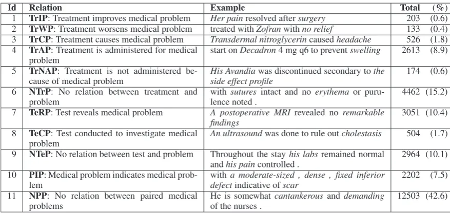
Eleven types of intra-sentential pairwise relations are annotated. A brief description of these relation types and the relevant statistics are provided in Table 1. As we can see from the table, each medical relation has atypeand is defined only onintra-sentenceTREATMENT-PROBLEM, TEST-PROBLEM, and
PROBLEM-PROBLEM concept pairs. Also, while there are 11 relation types, three of them, namely
Relations 6, 9, and 11, denote the absence of a medical relation between the corresponding concepts. The purpose of having “no relation” classes is to ensure that every pair of TEST/PROBLEM/TREATMENT
concepts is annotated, whether or not a medical relation exists between them.
3 Baseline MR Classification Systems
We employ two supervised MR classification systems as baselines. The first baseline is a state-of-the-art system that achieved the best performance in the official 2010 i2b2 evaluation. The second baseline is a tree kernel-based system, motivated by the fact that tree kernels are frequently used in relation extraction (e.g., Zhou et al. (2007), Zhu et al. (2013)).
3.1 SVM with Flat Features
Our first baseline, Rink et al.’s (2011) system, employs an SVM classifier trained on a set offlatfeatures (i.e., features that are discrete- or real-valued).
Following Rink et al., we create training instances as follows. First, we form training instances be-tween every pair of (PROBLEM, TEST, and TREATMENT) concepts in the training documents, labeling
Id Relation Example Total (%) 1 TrIP: Treatment improves medical problem Her painresolved aftersurgery 203 (0.6) 2 TrWP: Treatment worsens medical problem treated withZofranwithno relief 133 (0.4) 3 TrCP: Treatment causes medical problem Transdermal nitroglycerincausedheadache 526 (1.8) 4 TrAP: Treatment is administered for medical
problem start onDecadron4 mg q6 to preventswelling 2613 (8.9) 5 TrNAP: Treatment is not administered
be-cause of medical problem His Avandiaside effect profilewas discontinued secondary tothe 174 (0.6)
6 NTrP: No relation between treatment and
problem withlence noted .sutures intact and no erythemaor puru- 4462 (15.2) 7 TeRP: Test reveals medical problem A postoperative MRI revealed no remarkable
findings 3051 (10.4)
8 TeCP: Test conducted to investigate medical
problem An ultrasoundwas done to rule outcholestasis 504 (1.7) 9 NTeP: No relation between test and problem Throughout the stayhis labs remained normal
andhis paincontrolled . 2964 (10.1)
10 PIP: Medical problem indicates medical
prob-lem withdefecta moderate-sized , dense , fixed inferiorindicative ofscar 2202 (7.5)
11 NPP: No relation between paired medical
[image:3.595.77.516.60.268.2]problems He is somewhatof the nurses . cantankerous and demanding 12503 (42.6)
Table 1: The 11 relation types for medical relation classification. Each relation type is defined on an ordered pair where concepts in the pair are as specified by the relation. The “Total” and “%” columns show the number and percentage of instances annotated with the corresponding relation type over all 426 discharge summaries, respectively.
instances belonging to the three “no relation” classes.2 Specifically, we downsample the instances be-longing to the three “no relation” classes (i.e.,NTrP,NTeP, andNPP) by ensuring that (1) the ratio of the number ofNTrPinstances to the number of TREATMENT-PROBLEM instances is 0.06; (2) the ratio
of the number ofNTePinstances to the number of TEST-PROBLEM instances is 0.03; and (3) the ratio
of the number ofNPPinstances to the number of PROBLEM-PROBLEMinstances is 0.5. These ratios are
selected using our 30-summary development set, as described in Section 2. As mentioned above, each instance corresponds to a pair of concepts,c1 andc2, and is represented using 37 groups of features that can be divided into five categories:3
Context (13 groups). The words, the POS tags, the bigrams, the string of words, the sequence of phrase chunk types, and the concept types used betweenc1 andc2; the word precedingc1/c2; any of the
three words succeedingc1/c2; the predicates associated withc1/c2; the predicates associated with both concepts; and a feature that indicates whether a conjunction regular expression matched the string of words betweenc1andc2.
Similarity (5 groups). We find the concept pairs in the training set that are most similar to the (c1,c2)
pair (i.e., its nearest neighbors), and create features that encode the statistics collected from these nearest neighbors. To find the nearest neighbors, we (1) represent each pair in the training set as a sequence; (2) define the number of nearest neighbors to use; and (3) define a similarity metric to compute the similarity of two sequences.
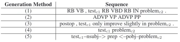
Following Rink et al. (2011), we employ five methods to represent a pair. The five methods are: (1) as a sequence of POS tags for the entire sentence containing the pair; (2) as a phrase chunk sequence between the two concepts; (3) as a word lemma sequence beginning the two words before the first concept, up to and including the second word following the second concept in the pair; (4) as a concept type sequence for all the concepts found in the sentence containing the pair; and (5) as a shortest dependency path sequence connecting the two concepts. Table 2 shows an example of these five methods of generating sequences from the TESTconcepther examand the PROBLEMconcepther hyperreflexiain the sentence
2Other methods for addressing class imbalance, such as over-sampling (Chawla et al., 2002) and cost-sensitive learning
(Turney, 1995), can also be employed.
3To compute the features, we use (1) the Stanford CoreNLP tool (Manning et al., 2014) to obtain POS tags, word lemmas,
Generation Method Sequence
(1) RB VB , testc1RB VBD RB IN problemc2.
(2) ADVP VP ADVP PP
(3) postop , testc1only improve slightly in problemc2.
(4) testc1problemc2
[image:4.595.156.444.60.128.2](5) testc1–nsubj–>prep<–pobj–problemc2
Table 2: Examples of the five methods of sequence generation.
Postop, her exam only improved slightly in her hyperreflexia . Note that for better generalization, the two concepts are replaced with their concept type (i.e., her exam and her hyperreflexia are replaced with testc1 and problemc2 respectively) before sequence generation. Like Rink et al., we seek different
numbers of nearest neighbors for the five methods of generating sequences. For the first method, we use 100 nearest neighbors; for the second method, 15 neighbors; for the third method, 20 neighbors; for the fourth method, 100 neighbors; and for the fifth method, 20 neighbors. We use the Levenshtein distance (Levenshtein, 1966) as the similarity metric.
After finding the nearest neighbors for each of the five methods of sequence representation, we create features as follows. For each method, we compute the percentage of nearest neighbors belonging to each of the 11 relation types, and then create 11 features whose values are these 11 numbers.
Single concept (11 groups).Any word lemma fromc1/c2; any word used to describec1/c2; the concept type forc1/c2; the string of words inc1/c2; the concatenation of assertion types for both concepts; and the
sentiment category (i.e., positive or negative) ofc1/c2obtained from the General Inquirer lexicon (Stone
et al., 1968).
Wikipedia (6 groups). Six features are computed based on the Wikipedia articles, their categories, and the links between them. The first feature encodes whether neither c1 norc2 contains any substring that
may be matched against the title of an article. The second feature encodes whether the links between the articles retrieved based on the two concepts are absent. The next two features encode whether a link exists from the article pertaining toc1 (c2) to the article pertaining toc2 (c1). The fifth feature encodes
whether there are links between the articles pertaining to both concepts. The last feature encodes whether both concepts have the same concept type according to their Wikipedia categories.
Vicinity (2 groups). The concatenation of the type ofc1 and the type of the closest concept preceding c1; and the concatenation of the type ofc2and the type of the closest concept succeedingc2.
After creating the training instances, we train a 11-class classifier on them using SVMmulticlass (Tsochantaridis et al., 2004). We set C, the regularization parameter, to 10,000, since preliminary exper-iments indicate that preferring generalization to overfitting (by setting C to a small value) tends to yield poorer classification performance. The remaining learning parameters are set to their default values. Af-ter training, we use the resulting classifier to make predictions on the test instances, which are generated in the same way as the training instances.
3.2 SVM with Structured Feature
In this framework, each instance is represented using a single structured feature computed from the parse tree of the sentence containing the concept pair. Since publicly available SVM learners capable of handling structured features can only make binary predictions, we train 11 SVM classifiers, one for representing each medical relation. In each classifier’s training data, a positive instance is one whose class value matches the medical relation class value of the classifier, and a negative instance is one with other class values applicable to the given concept pair. Since the negative instances significantly out-number the positive instances in each of these binary classifiers, we reduce data skew by downsampling the negative instances. Following the order of the 11 relations listed in Table 1, the optimal ratios of negative-to-positive instances according to our 30-summary development set are 0.2, 0.2, 0.06, 0.2, 0.5, 1, 1, 0.3, 0.06, 0.06, and 0.09, respectively. We set C to 100 based on the development data.
representation of the syntactic context of the two concepts than using apartialparse tree, the increased complexity of the tree also makes it more difficult for the SVM learner to make generalizations.
To strike a better balance between having a rich representation of the context and improving the learner’s ability to generalize, we extract a subtree from a parse tree and use it as the value of the struc-tured feature of an instance. Specifically, given two concepts in an instance and the associated syntactic parse treeT, we retain as our subtree the portion ofT that covers (1) all the nodes lying on the shortest path between the two entities, and (2) all the immediate children of these nodes that are not the leaves of
T. This subtree is known as a simple expansion tree.
After training the 11 tree kernel-based relation classifiers, we can apply them to classify a test instance. The class value of an instance is determined based on the classifier with the maximum classification confidence, where the confidence value of an instance is its signed distance from the SVM hyperplane.
4 Exploiting Sequences for MR Classification
Unlike the two baselines, which exploit flat features and parse-based structured features for MR classifi-cation, in this section we describe three MR classification systems that exploit sequences.
4.1 Dependency-Based Sequences
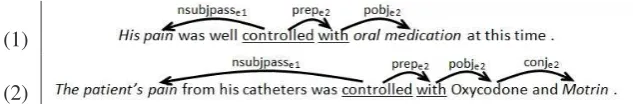
The first system is based on sequences ofdependencyrelations. To see why dependency relations could be useful for MR classification, consider the sentences in Table 3:
(1)
[image:5.595.143.460.347.399.2](2)
Table 3: Example dependency paths.
In sentences (1) and (2), the PROBLEMconceptsHis painandThe patient’s painoccur as the subject
of the verb controlled and the TREATMENTconceptsoral medicationandMotrinoccur as objects of the
prepositional with modifier of the same verb controlled. In other words, intuitively, the verb controlled cues that the PROBLEMconcept is being controlled, and together with the preposition with it cues that the
TREATMENTconcept is doing the controlling. Note that in each case the relation between the PROBLEM
and TREATMENTisTrIP, which can now be easily inferred given the dependency relations of the concept
pairs with the verb controlled. These examples suggest that the verb closest to each of the two concepts is an important word as it cues the relation.
Given the usefulness of dependency structures and the verb closest to each concept for MR classifica-tion, we represent each training/test instance as a paired dependency sequence with separate dependency paths traced from each concept in the pair to its closest verb. To reduce data sparsity, for the argument words found in a dependency path, we replace them with their POS tags. For example, given sentence (1), the path extracted fromHis painis “nsubjpass ( controlled NN )” and fromoral medication is “prep ( controlled with ) pobj ( with NN )”.4
Next, we describe how to classify a test instanceinst. First, we identify the set of training instancesT
that satisfy two conditions: (a) the ancestor verb pair in the training instance is the same as that ininst, and (b) each of the two dependency sequences in the training instance either is the same as, or contains, or is contained in the corresponding dependency sequences ininst. Second, we find forinst its nearest neighbor inT by employing the following similarity function:
Similarity(train, test) =cosine(pathtrainc1, pathtestc1)·cosine(pathtrainc2, pathtestc2) (1)
4Note that sometimes a dependency path cannot be traced (e.g., a verb does not exist, which is not uncommon in a discharge
wherecosine(x,y) is a function that computes the cosine similarity ofxandy.5 Finally, if the similarity between inst and its nearest neighbor inT is greater than a threshold, we classify inst using the class value of its nearest neighbor.6 Otherwise, this system will leaveinst unclassified. In other words, this system is precision-oriented, classifying only those instances it can classify confidently.
4.2 Lexical Patterns
In our second system, we represent each concept pair as a lexical pattern. Specifically, we employ Generation Method 3 as described in the Similarity features in Section 3.1 to generate a lexical pattern from a concept pair. To classify a test instanceinst, we employ the one-nearest-neighbor algorithm. To identify the nearest neighbor ofinst, we employ the Levenshtein distance as the similarity metric.
Two questions naturally arise. First, since these lexical patterns have already been used to generate features in the flat-feature baseline, why do we still employ them in a separate system? To answer this question, note that although these lexical patterns were used to generate features for training the flat-feature baseline classifier, we have no control over whether these features are deemed useful by the learning algorithm and are subsequently used by the resulting classifier. Having a separate system that employs these patterns ensures that they will be used when making the final classification decision.
Second, given that we described five methods to generate sequences in Section 3.1, why do we employ Generation Method 3 but not the remaining methods? In principle, we can employ the remaining four generation methods for generating lexical patterns as well: all we need to do is to create four additional systems, each of which makes use of the patterns created by exactly one of the four methods. In prac-tice, however, not all generation methods are equally good: if a method does not generate patterns that adequately capture context, then employing the resulting patterns may yield poor-performing systems. Consequently, we employ only the system corresponding to the generation method that yields the best performance on the development data, which turns out to be the system corresponding to Method 3.
4.3 Rules
In the previous subsection, we employ automatically induced patterns. In contrast, our third system em-ploys patterns that arehand-craftedbased on manual observations made on thetrainingset. Specifically, we ask a human to identify the contexts of two concepts that are strongly indicative of a relation class. Like the automatically induced patterns, each hand-crafted pattern is composed of the types of the two concepts involved and the context in which they occur. For example, in the patterndue toPROBLEMby
TREATMENT, the TREATMENTis likely to cause the PROBLEMand therefore it will be labeled asTrCP.
As another example, in the patternattributed toPROBLEMas a result ofPROBLEM, the two PROBLEMs
are likely to have an indicative relation and therefore it will be labeled asPIP. At the end of this process, we end up with 136 manually labeled patterns, which we will subsequently refer to as aruleset.
Next, we order these rules in decreasing order of accuracy, where the accuracy of a rule is defined as the number of times it yields the correct MR type divided by the number of times it is applied, as measured on the training set.
Given this ruleset, we can classify a test instance using the first applicable rule in it. If no rules are applicable, the test instance will remain unclassified.7
5 The Ensemble
In the previous section, we described three systems for MR classification. Together with the two baseline systems, we have five systems for MR classification. A natural way to make use of all of them for MR classification is to include them in an ensemble. The question, then, is: how do we classify a test instance using this ensemble? The simplest approach is perhaps majority voting, but that presumes that each
5To apply cosine similarity, we represent each path as a frequency-count vector, where each dimension in the vector
corre-sponds to a dependency type or an argument word appearing in the path.
6Based on development set experiments, the similarity threshold values for each concept pair type are:T
T reatment−P roblem
= 0.85;TT est−P roblem= 0.75; andTP roblem−P roblem= 0.75.
7Space limitations preclude a complete listing of these rules. See our website athttps://www.hlt.utdallas.edu/
member of the ensemble is equally important. In practice, however, some members are more important than the others, so the votes cast by these members should have higher weights.
To model this observation, we combine the (probabilistic) votes of the members in a weighted fashion using the following formula:
Pcombined(c) =w1·Ptree(c) +w2·Pflat(c) +w3·Pdependency(c) +w4·Pword(c) +w5·Prules(c) (2) where wi (i = 1, . . . ,5) is a combination weight, and Px(c) is the probability that the test instance belongs to classcaccording to systemx.
Two questions naturally arise. First, how can the combination weights be determined? We perform an exhaustive search on held-out development data to find the combination of weights that jointly maximizes overall accuracy on the development set. We allow each weight to vary between 0 and 1 in steps of 0.1, subject to the constraint that the five weights sum to 1.
Second, how canPx(c)be computed? In other words, how can each system compute the probability that a given test instance belongs to a certain class? To answer this question, we have to convert the output of each system for each test instance into a 11-element probability vector, which is used to encode the probability that the given test instance belongs to each of the 11 relation types.
We perform the conversion as follows. For the two baseline systems, the SVM outputs a confidence value for each class. Hence, to obtain the probability vector, we first normalize the confidence value associated with each class so that it falls within the [0,1] range, and then normalize the resulting values so that they sum to 1. For the systems employing lexical patterns and dependency-based sequences, the class chosen by each system receives a probability of 0.6, and each of the other classes applicable to the test instance under consideration receives an equal share of the remaining probability mass. For the rule-based system, we take the rule that is used to classify the test instance and apply this rule to each instance in the training set to estimate the probability that the rule is correct with respect to each of the 11 classes. We can then use the resulting 11 probabilities to create the 11-element probability vector.
Finally, recall that some of these systems are not applicable to all of the test instances. If this happens, the corresponding system(s) will return a vector in which all of its elements are set to 0.
6 Enforcing Global Consistency
So far we have had an ensemble that, given a test instance, returns the probability that it belongs to each of the 11 classes. Since the test instances are classified independently of each other, there is no guarantee that the resulting classifications are globallyconsistent. To enforce global consistency, we employ global constraints implemented in the Integer Linear Programming (ILP) framework (Roth and Yih, 2004).
Since our constraints are intra-sentential, we formulate one ILP program for each sentencesin each training summary. Each ILP program contains11×Nsvariables, whereNsis the number of test instances formed from the concept pairs ins. In other words, there is one binary indicator variablexi,j,r for each relation classrof each test instanceinstformed from conceptiand conceptj, which will be set to 1 by the ILP solver if and only if it thinksinstshould belong to classr.
Our objective is to maximize the linear combination of these variables and their corresponding proba-bilities given by the ensemble (see (3) below) subject to two types of constraints, theintegrityconstraints and the consistencyconstraints. The integrity constraints ensure that each concept pair is assigned ex-actly one relation type (see the equality constraint in (4)). The consistency constraints ensure consistency between the predictions made for different instances in the same sentence.
Maximize:
X
(i,j)∈R
X
r∈L
pi,j,rxi,j,r (3)
subject to:
X
r∈L
Relation Relations in Conflict
TrIP(tri,pj) TrWP(tri,pk),TrCP(tri,pm),TrNAP(tri,pn)
TrWP(tri,pj) TrIP(tri,pk),TrCP(tri,pm),TrNAP(tri,pn)
TrCP(tri,pj) TrIP(tri,pk),TrWP(tri,pm),TrNAP(tri,pn)
TrAP(tri,pj) TrNAP(tri,pk)
TrNAP(tri,pj) TrAP(tri,pk),TrIP(tri,pm),TrWP(tri,pn),TrCP(tri,po)
TeRP(tei,pj) TeCP(tei,pk)
[image:8.595.156.442.60.142.2]TeCP(tei,pj) TeRP(tei,pk)
Table 4: Constraints on relation types.
and consistency constraints.
Note that (1) pi,j,r is the probability that the instance formed from concept iand concept j belongs to relation typeraccording to the ensemble; (2)Ldenotes the set of unique relation types; and (3)Ris the set of instances in the sentence under consideration.
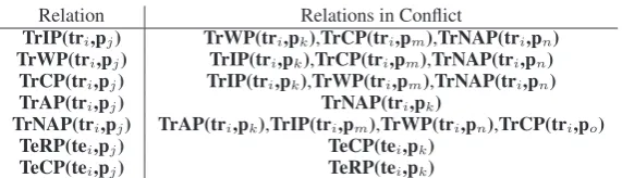
The consistency constraints are listed in Table 4. Each row of the table represents a constraint and can be interpreted as follows. If the relation in the first column holds, then none of the relations in the second column can hold. Consider, for instance, the constraint in the first row of the table, which says that if TREATMENTtriimproves PROBLEMpj, thentricannot worsen, cause, or be administered for any other PROBLEM. At first glance, it may not seem intuitive that a treatment that improves one problem cannot
also worsen or cause other problems. This can be attributed to the way a patient discharge summary is written: while the constraint can be violated for concept pairs indifferentsentences, there is no case in which the constraint is violated for concept pairs in the same sentence in the training set. These constraints can be implemented as linear constraints in ILP. For example, the constraint “if TREATMENT triimproves PROBLEMpj, thentricannot worsen PROBLEMpk” can be implemented as follows.
xi,j,TrIP≤1−xi,k,TrWP (5)
7 Evaluation
7.1 Experimental Setup
Following the 2010 i2b2/VA evaluation scheme, we assume that (1) gold concepts and their types are given, and (2) a medical relation classification system is evaluated on all but the “no relation” types. In other words, a system will not bedirectlyrewarded if it correctly identifies a “no relation” instance, but will be penalized if it misclassifies a “no relation” instance as one of the eight relation types.
As mentioned before, we use 170 training summaries from the 2010 i2b2/VA corpus for classifier training and reserve 256 test summaries for evaluating system performance. Thirty training summaries are used for development purposes in all experiments that require parameter tuning.
7.2 Results and Discussion
Table 5 shows the 8-class classification results for our MR classification task, where results are expressed in terms of recall (R), precision (P), and micro F-score (F).
Row 1 and row 2 show the results of the flat-feature baseline and the structured-feature baseline, respectively. As we can see, the flat-feature baseline performs significantly better than the structured-feature baseline.8 It is worth mentioning that since the dataset available to the research community which we are using contains a subset of the summaries from the dataset that was available to the shared task participants, we were unable to directly compare our system’s performance with theirs. Nevertheless, we believe that the results of our reimplementation of Rink et al.’s (2011) system in row 1 can be taken to be roughly the state of the art results on this dataset.
Rows 3–5 show the results of the three systems we introduced. As we can see from row 3, by using simple lexical patterns in combination with the Levenshtein similarity metric, we achieve an F-score that is significantly better than that of the structured-feature baseline but significantly worse (atp < 0.01) than
Individual System R P F
1 Flat 66.7 58.1 62.1
2 Tree 64.3 55.6 59.6
3 Lexical Patterns 63.9 59.2 61.4 4 Dependencies 4.3 82.9 8.2
5 Rules 11.9 84.4 9.1
Ensemble System R P F
6 Ensemble(1+2) 69.2 61.3 65.0
7 Ensemble(1+2+3) 70.4 63.1 66.6
8 Ensemble(1+2+3+4) 70.0 64.7 67.2
9 Ensemble(1+2+3+4+5) 71.1 64.8 67.8
10 Ensemble(1+2+3+4+5)+ ILP 72.9 66.7 69.6
Single Classifier R P F 11 Single(1+2) 53.0 73.6 61.7
12 Single(1+2+3) 54.4 74.7 63.0
13 Single(1+2+3+4) 56.4 73.7 63.9
14 Single(1+2+3+4+5) 56.3 74.5 64.1
15 Single(1+2+3+4+5)+ ILP 58.9 75.0 66.0
Bagged System R P F
16 Bagging(1+2) 54.6 73.6 62.7
17 Bagging(1+2+3) 54.5 73.8 62.7
18 Bagging(1+2+3+4) 56.9 73.2 64.0
19 Bagging(1+2+3+4+5) 56.7 73.9 64.2
[image:9.595.80.517.61.192.2]20 Bagging(1+2+3+4+5)+ ILP 59.2 75.5 66.4
Table 5: Medical relation classification results.
that of the flat-feature baseline. On the other hand, the remaining two systems are precision-oriented: they classify an instance only if they can do so confidently, thus resulting in poor recall.
Rows 6–10 show the results of our ensemble approach when the individual MR classification systems are added incrementallyto the flat-feature baseline. Except for the addition of the dependency-based system and the hand-crafted rules, which yielded insignificant improvements in F-score, the addition of all other components yielded significant improvements. In fact, every significant improvement in F-score is accompanied by a simultaneous rise in recall and precision. The best-performing system is the one that comprises all of our components, achieving an F-score of 69.6. This translates to a relative error reduction of 19.8% and a highly significant improvement (p < 0.001) over our reimplementation of Rink et al.’s (2011) state-of-the-art baseline. The weights learned for the members of the ensemble are indeed different: both baselines have a weight of 0.3, the rule-based system and the lexical patterns have a weight of 0.1, and the remaining weight goes to the dependency-based component.
7.3 Additional Comparisons
Given the above results, a natural question is: is an ensemble approach ever needed to combine the knowledge sources exploited by different systems in order to obtain these improvements? In other words, can we achieve similar performance by training asingleclassifier using a feature set containing all the features currently exploited by different members of the ensemble?
To answer this question, we repeat the experiments in rows 6–10 of Table 5, except that in each ex-periment we train a single classifier on a feature set formed from the union of those features employed by all the members of the corresponding ensemble. Results are shown in rows 11–15 of Table 5. In each of these five experiments the F-score obtained by our ensemble approach is significantly better than that achieved by the corresponding single-classifier approach. In addition, although we see improvements in F-score as we add the individual extensions (including ILP) incrementally to the flat-feature base-line, none of these improvements is statistically significant. Nevertheless, when applied in combination, these extensions yield a system that is significantly better than the flat-feature baseline. Overall, these results provide suggestive evidence that to achieve the same level of performance we cannot replace our ensemble approach with a simpler setup that relies on a single classifier.
Given that our ensemble approach performs better than a single-classifier approach, a relevant question is: do we have to useourensemble approach, or can we still achieve similar performance by replacing it with a generic ensemble learning method such asbagging(Breiman, 1996)?
is significantly worse that that achieved by our ensemble approach. In fact, comparing bagging and the single-classifier approach, their results are statistically indistinguishable in all but one case (row 11 vs. row 16), where bagging achieves significantly better performance. Like in the single-classifier experi-ments, in the bagging experiments we see improvements in F-score as we add the individual extensions (including ILP) incrementally to the flat-feature baseline, although the improvements are significant only with the addition of ILP and the dependency-based system. Nevertheless, when applied in combination, these extensions yield a system that is significantly better than the flat-feature baseline. Overall, these results provide suggestive evidence that to achieve the same level of performance we cannot replace our ensemble approach with bagging.
8 Error Analysis
To gain additional insights into our ensemble approach and to provide directions for future work, we conduct an error analysis of our best-performing system.
NTeP confused as TeRP.This is a frequent type of confusion where 34% of the TEST–PROBLEM pairs
that do not have a relation are misclassified as having a “Test Reveals Problem” relation. Below are two subcategories of errors commonly made by the system in this confusion category.
• TESTwith numeric results followed byPROBLEMconcepts in written text
The following example illustrates this confusion:
. . . [test mean gradient] 33 mm , [problem decreased disc motion] , [problem mobile mass in LVOT] , [problemmild AI] , [problemmild to moderate MR] . . .
In sentences like the one above where a TEST concept has a numeric result (result of TEST mean gradientis33 mm), since the TESTconcept is already associated with its result, it has no relation with
any other concepts in the sentence. While in some cases the system is able to correctly classify the relation between the TESTconcept and the first following PROBLEMconcept, in almost all cases, it fails
to propagate this no relation class down through the other PROBLEMs listed in a series following the
TESTconcept. For the sentence above, it incorrectly classifies the relation between TESTconceptmean gradientand each of the PROBLEMconceptsmobile mass in LVOT,mild AI, andmild to moderate MR
asTeRPinstead ofNTeP.
• TESTrevealsPROBLEMthat is consistent with otherPROBLEM
This is a common error where a TEST concept is classified as revealing two consistent PROBLEM
concepts when in actuality it only reveals one of the PROBLEMs. Consider the following sentence:
[testRadiograph] revealed [problembilateral diffuse granular pattern] consistent with [problemsurfactant
deficiency] .
In this sentence, PROBLEMconceptbilateral diffuse granular patternis described as being consistent
with another PROBLEMconceptsurfactant deficiency. While the system correctly classifies the pair ( Ra-diograph, bilateral diffuse granular pattern) asTeRP, it misclassifies the pair (Radiograph, surfactant deficiency) asTeRP. In case of the second pair, the TEST concept has no relation with the PROBLEM
concept. From this common error type, an insight one can derive is that the system is currently missing knowledge of the association of the two PROBLEMs w.r.t. each other, and thus in turn cannot make an
informed decision of which of the two PROBLEMs the TESTconcept actually reveals.
PIP confused as NPP. The second major confusion in the system’s output concerns misclassifying PROBLEMconcept pairs that are indicative of each other as having “no relation”. We observe that 39.5%
of thePIPinstances get classified asNPP.
• PROBLEMwithout anotherPROBLEM
In a sentence, if a PROBLEMconcept is actually said to be without another PROBLEM, then such a pair is
commonly misclassified by the classifier into the no-relation classNPPinstead of the has-relation class
both conceptsbleedingand drainage, respectively. Such cases call for domain-specific knowledge that can aid in identifying attributes of PROBLEMs, like that the PROBLEM conceptsbleedinganddrainage
are commonly associated attributes of the PROBLEM concept Angio site. With this information the
system is better equipped to recognize that PROBLEMAngio siteis related to its attributes. 9 Conclusion
We investigated a new approach to the medical relation classification task, where we employed human-supplied knowledge to assist the construction of relation classification systems based on sequences, com-bined them via an ensemble, and then enforced global consistency using constraints in an ILP framework. Experimental results on the i2b2 corpus show a significant relative error reduction of 19.8% over a state-of-the-art baseline.
Acknowledgments
We thank the three anonymous reviewers for their detailed and insightful comments on an earlier draft of this paper. This work was supported in part by NSF Grants IIS-1147644 and IIS-1219142.
References
Eugene Agichtein and Luis Gravano. 2000. Snowball: Extracting relations from large plain-text collections. In
Proceedings of the Fifth ACM Conference on Digital Libraries, pages 85–94.
Michele Banko, Michael Cafarella, Stephen Soderland, Matthew Broadhead, and Oren Etzioni. 2007. Open information extraction for the Web. InProceedings of the 20th International Joint Conference on Artificial Intelligence, pages 2670–2676.
Kurt Bollacker, Colin Evans, Praveen Paritosh, Tim Sturge, and Jamie Taylor. 2008. Freebase: A collabora-tively created graph database for structuring human knowledge. InProceedings of the 2008 ACM SIGMOD International Conference on Management of Data, pages 1247–1250.
Leo Breiman. 1996. Bagging predictors.Machine Learning, 24:123–140.
Sergey Brin. 1999. Extracting patterns and relations from the World Wide Web. InThe World Wide Web and Databases, pages 172–183. Springer.
Razvan Bunescu and Raymond Mooney. 2007. Learning to extract relations from the Web using minimal su-pervision. InProceedings of the 45th Annual Meeting of the Association for Computational Linguistics, pages 576–583.
Nitesh V. Chawla, Kevin W. Bowyer, Lawrence O. Hall, and W. Philip Kegelmeyer. 2002. SMOTE: Synthetic minority over-sampling technique.Journal of Artificial Intelligence Research, 16:321–357.
Ronan Collobert, Jason Weston, L´eon Bottou, Michael Karlen, Koray Kavukcuoglu, and Pavel P. Kuksa. 2011. Natural language processing (almost) from scratch.Journal of Machine Learning Research, 12:2493–2537. Berry de Bruijn, Colin Cherry, Svetlana Kiritchenko, Joel Martin, and Xiaodan Zhu. 2011. Machine-learned
solutions for three stages of clinical information extraction: The state of the art at i2b2 2010. Journal of the American Medical Informatics Association, 18(5):557–562.
Oren Etzioni, Michael Cafarella, Doug Downey, Ana-Maria Popescu, Tal Shaked, Stephen Soderland, Daniel S Weld, and Alexander Yates. 2005. Unsupervised named-entity extraction from the Web: An experimental study.Artificial Intelligence, 165(1):91–134.
Sebastian Krause, Hong Li, Hans Uszkoreit, and Feiyu Xu. 2012. Large-scale learning of relation-extraction rules with distant supervision from the Web. InProceedings of the International Semantic Web Conference, pages 263–278.
Vladimir I. Levenshtein. 1966. Binary codes capable of correcting deletions, insertions and reversals. Soviet Physics Doklady, 10(8):707–710.
Christopher D. Manning, Mihai Surdeanu, John Bauer, Jenny Finkel, Steven J. Bethard, and David McClosky. 2014. The Stanford CoreNLP Natural Language Processing Toolkit. InProceedings of the 52nd Annual Meet-ing of the Association for Computational LMeet-inguistics: System Demonstrations, pages 55–60.
Mike Mintz, Steven Bills, Rion Snow, and Daniel Jurafsky. 2009. Distant supervision for relation extraction without labeled data. InProceedings of the Joint Conference of the 47th Annual Meeting of the ACL and the 4th International Joint Conference on Natural Language Processing of the AFNLP, pages 1003–1011.
Truc Vien T. Nguyen and Alessandro Moschitti. 2011. End-to-end relation extraction using distant supervision from external semantic repositories. InProceedings of the 49th Annual Meeting of the Association for Compu-tational Linguistics: Human Language Technologies, pages 277–282.
Patrick Pantel and Marco Pennacchiotti. 2006. Espresso: Leveraging generic patterns for automatically harvesting semantic relations. InProceedings of the 21st International Conference on Computational Linguistics and the 44th Annual Meeting of the Association for Computational Linguistics, pages 113–120.
Deepak Ravichandran and Eduard Hovy. 2002. Learning surface text patterns for a question answering system. In
Proceedings of the 40th Annual Meeting on Association for Computational Linguistics, pages 41–47.
Ellen Riloff and Rosie Jones. 1999. Learning dictionaries for information extraction by multi-level bootstrapping. InProceedings of the Sixteenth National Conference on Artificial Intelligence, pages 474–479.
Bryan Rink, Sanda Harabagiu, and Kirk Roberts. 2011. Automatic extraction of relations between medical concepts in clinical texts.Journal of the American Medical Informatics Association, 18(5):594–600.
Dan Roth and Wen-tau Yih. 2004. A linear programming formulation for global inference in natural language tasks. InProceedings of the Eighth Conference on Computational Natural Language Learning, pages 1–8. Benjamin Rozenfeld and Ronen Feldman. 2008. Self-supervised relation extraction from the Web. Knowledge
and Information Systems, 17(1):17–33.
Yusuke Shinyama and Satoshi Sekine. 2006. Preemptive information extraction using unrestricted relation dis-covery. InProceedings of the Human Language Technology Conference of the North American Chapter of the Association for Computational Linguistics, pages 304–311.
Philip J. Stone, Dexter C. Dunphy, Marshall S. Smith, and Daniel M. Ogilvie. 1966. The General Inquirer: A Computer Approach to Content Analysis. MIT Press, Cambridge, Massachusetts.
Fabian M. Suchanek, Gjergji Kasneci, and Gerhard Weikum. 2007. YAGO: A core of semantic knowledge. In
Proceedings of the 16th International World Wide Web Conference, pages 697–706.
Mihai Surdeanu and Massimiliano Ciaramita. 2007. Robust information extraction with perceptrons. In Proceed-ings of the NIST 2007 Automatic Content Extraction Workshop.
Ioannis Tsochantaridis, Thomas Hofmann, Thorsten Joachims, and Yasemin Altun. 2004. Support vector machine learning for interdependent and structured output spaces. InProceedings of the 21st International Conference on Machine Learning, pages 104–112.
Peter Turney. 1995. Cost-sensitive classification: Empirical evaluation of a hybrid genetic decision tree induction algorithm.Journal of Artificial Intelligence Research, 2:369–409.
¨Ozlem Uzuner, Brett R South, Shuying Shen, and Scott L DuVall. 2011. 2010 i2b2/VA Challenge on concepts, assertions, and relations in clinical text.Journal of the American Medical Informatics Association, 18(5):552– 556.
GuoDong Zhou, Jian Su, Jie Zhang, and Min Zhang. 2005. Exploring various knowledge in relation extraction. InProceedings of the 43rd Annual Meeting of the Association for Computational Linguistics, pages 427–434. GuoDong Zhou, Min Zhang, DongHong Ji, and QiaoMing Zhu. 2007. Tree kernel-based relation extraction with
context-sensitive structured parse tree information. InProceedings of the 2007 Joint Conference on Empirical Methods in Natural Language Processing and Computational Natural Language Learning, pages 728–736. Xiaodan Zhu, Colin Cherry, Svetlana Kiritchenko, Joel Martin, and Berry de Bruijn. 2013. Detecting concept