A Fast Accurate Two-stage Training Algorithm for
L1-regularized CRFs with Heuristic Line Search Strategy
Jinlong Zhou
Fudan University Shanghai, China
Xipeng Qiu
Fudan University Shanghai, China
Xuanjing Huang
Fudan University Shanghai, China
Abstract
Sparse learning framework, which is very popular in the field of nature language processing recently due to the advantages of efficiency and generalizability, can be applied to Conditional Random Fields (CRFs) with L1 regularization method. Stochastic gradient descent (SGD) method has been used in training L1-regularized CRFs, because it often requires much less training time than the batch training algo-rithm like quasi-Newton method in prac-tice. Nevertheless, SGD method some-times fails to converge to the optimum, and it can be very sensitive to the learn-ing rate parameter settlearn-ings. We present a two-stage training algorithm which guar-antees the convergence, and use heuris-tic line search strategy to make the first stage of SGD training process more robust and stable. Experimental evaluations on Chinese word segmentation and name en-tity recognition tasks demonstrate that our method can produce more accurate and compact model with less training time for L1 regularization.
1 Introduction
Conditional Random Fields (CRFs) (Lafferty et al., 2001; Sutton and McCallum, 2006) are one of the most widely-used machine learning approach in the field of nature language processing, for their ability to handle large feature sets and structural dependency between output labels. The applica-tions of CRFs cover a wide range of tasks such as part-of-speech (POS) tagging (Lafferty et al., 2001), semantic role labeling (Toutannova et al., 2005) and syntactic parsing (Finkel et al., 2008). CRFs outperform other models like Maximum En-tropy Markov models (McCallum et al., 2000), be-cause they overcome the problem of “label bias”.
Moreover, CRFs can output the probabilistic of la-beling result for further use as pipeline or rerank-ing.
For all types of CRFs, the maximum-likelihood method can be applied for parameter estimation, which means training the model is done by max-imizing the log-likelihood on the training data. To avoid overfitting the likelihood is often penal-ized with the regularization term. There were two common regularization methods named L1 and L2 regularization. L1 regularization, also called Laplace prior, penalizes the weight vector with its L1-norm. L2 regularization, also called Gaussian prior, uses L2-form. Based on the work of Gao et al. (2007), there is no significant difference be-tween these two regularization methods in terms of accuracy. But L1 regularization has a major ad-vantage that L1-regularized training can produce models, of which the feature weights can be very sparse, then the size of the model will be much smaller than that produced by L2 regularization. Compact models are more interpretable, general-izable and manageable, require less resources like memory and storage. It is very meaningful espe-cially for the rapid development of mobile appli-cation nowadays, which suffer the scarcity of re-sources. In many NLP tasks, the feature sets can reach the magnitude of several million.
Besides, L1 regularization method can implic-itly perform the feature selection, and provide the result for further process such as iterative approach (Vail et al., 2007; Peng and McCallum, 2004). This task requires that we need to train the model as accurate as possible, as to converge to the op-timum. The feature selection can be regarded as reliable and unbiased after such a process.
Quasi-Newtion method was successfully and efficiently used in L1-regularized model by An-drew and Gao (2007). They presented an algorithm called Orthant-Wise Limited-memory Quasi-Newton (OWQN), which is based on
BFGS algorithm (Liu and Nocedal, 1989) and achieve better convergence than the method intro-duced by Kazama and Tsujii (2003).
Stochastic gradient descent (SGD) methods are another kind of L1-regularized training methods. It is a very attractive framework for it often re-quires much less training time than the batch train-ing algorithm in practice. Tsuruoka et al. (2009) presented a variant of SGD that can efficiently pro-duce compact models with L1 regularization. The main idea is to keep track of the total penalty and the penalty each weight has applied, so that the penalization smooth away the noisy gradient.
Although SGD method with cumulative penalty is very efficient, it sometimes fails to converge to the optimum, because the training process is usu-ally terminated at a certain number of iterations without explicit stop criteria as in quasi-Newton method. Another problem is that the training re-sult of SGD method is very sensitive to the param-eter settings of learning rate, therefore we have to tune the values of parameters for different tasks, which is not efficient in practice.
In this paper, we present a two-stage L1-regularized training algorithm to solve these two problems. In the first stage, we use the SGD method to get a relative good solution quickly. In the second stage, we use the OWL-QN method to improve the model which has been dealt with the SGD method. By this means we can fast get the accurate model. The learning rate scheduling in the first stage is done by heuristic line search, which makes the process more robust and stable.
Our experiments are conducted on two tasks, Chinese word segmentation and name entity recognition. We show that our method can pro-duce more accurate and compact model with less training time for L1 regularization. We also ver-ify that the result of SGD training method will be more robust when using the heuristic line search strategy.
The rest of the paper is organized as follows. Section 2 introduces the basics of CRFs. Sec-tion 3 describe the two-stage algorithm for L1-regularized models. Experimental results are shown in Section 4. We conclude the work in Sec-tion 5.
2 Conditional Random Fields
In this section, we briefly describe the basics of conditional random fields (CRFs) (Lafferty et al.,
2001; Sutton and McCallum, 2006) and introduce the definition of some concepts and parameters.
2.1 Linear-chain CRFs
CRFs defines the conditional probabilistic distri-bution over possible output sequencesyfor obser-vationxas following:
p(y|x) = 1
weight of the feature, andZ(x)is the
normaliza-tion factor defined by
Z(x) =X
The feature function can be divided into uni-gram features and biuni-gram features, here we simply rewritefk(x, yt, t) asfk(x, yt−1, yt, t) for
conve-nient.
2.2 Training
The maximum-likelihood method is a commonly used way applied for parameter estimation, which means we train the model by minimize the negated conditional log-likelihood L(λ) on the training
data:
To avoid overfitting, the likelihood is often penal-ized with the regularization term, which we will talk about in the later sections.
The partial derivative of L(λ) by the feature
weightsλkare given by
∂
whereEp(y|x)denotes the conditional expectation
under the model distribution:
Ep(y|x)fk(x, yt−1, yt, t) =
X
(y0,y)
Computing the conditional expectation directly is impractical for the large number of possible tag sequences, which is exponential in the length of the observation. Thus, a dynamic program-ming approach known as the Forward-Backward algorithm originally described for Hidden Markov models (Rabiner, 1989), is applied in a slightly modified form. For the forward recursions, we have
α0(⊥) = 1
αt+1(y) =Py0αt(y0) expnPKk=1λkfk(x, y0, y, t)
o
and for the backward recursion, we have
βT+1(>) = 1
βt(y0) =Pyβt+1(y) expnPKk=1λkfk(x, y0, y, t)
o
for0≤t≤T andy∈Y, where⊥and>are de-fined as special states for the begin and end of the sequence. Then the normalization factor is com-puted by
Z(x) =β0(⊥), (6)
and the conditional probabilities P(yt−1 =
y0, yt=y|x)are given by
3 L1 Regularization in CRFs 3.1 Regularization
The logarithmic loss functionL(λ)defined by (3)
is usually penalized with an additional regulariza-tion term, which prevents the model from overfit-ting the training data. There are two common reg-ularization methods named L1 and L2 regulariza-tion, in the case of L1 regularizaregulariza-tion, the term is defined as:
R(λ) =CX
k
|λk|, (7)
whereC is the regularization parameter that
con-trols the trade-off between fitting exactly the ob-servations and the L1-norm of the weight vector. This value is usually tuned by cross-validation or using the heldout data.
Now we can redefine the objective loss function as
L(λ) +R(λ). (8)
3.2 Orthant-Wise Limited-memory Quasi-Newton
It is not easy to use some common numerical opti-mization strategies such as limited memory BFGS (Liu and Nocedal, 1989) directly with L1 regular-ization, because the regularization term is not dif-ferentiable when the weight is zero.
A very efficient strategy called Orthant-Wise Limited-memory Quasi-Newton (OWL-QN) method is introduced in (Andrew and Gao, 2007). This algorithm is motivated by the observation that the L1 regularization term is differentiable when restricted to a set of points in which each coor-dinate never changes sign (called its “orthant”). Furthermore it is a linear function of its argu-ment, which means the second-order behavior of the regularized objective function on a given or-thant is determined by the log-likelihood compo-nent alone. Only a few steps of the standard L-BFGS algorithm have been changed in the OWL-QN method, and these differences are listed be-low:
1. The “pseudo-gradient” is used in place of the gradient.
2. The resulting search direction is constrained to match the sign pattern of the negated pseudo-gradient.
3. Each parameter is projected back onto the ini-tial orthant of the previous value during the line search.
Andrew and Gao (2007) proved that OWL-QN method is guaranteed to converge to a globally op-timal result.
3.3 Stochastic Gradient Descent
Stochastic gradient approaches use a small batch of the observations to get a crude approximation of the gradient of the objective function given by (3). The small batch size makes us possible to update the parameters more frequently than the origin gradient descent and speed up the conver-gence. Only considering the log-likelihood term, the updates have the following form
ˆ
wherejis the iteration counter andηj is the
but the crude approximation from small randomly-selected subset of the training samples. In (Tsu-ruoka et al., 2009), a variant of SGD that can effi-ciently train L1-regularized CRFs was presented. The main idea can be concluded as follows:
1. Only update the weights of the features that are used in the current observation, called “lazy update”.
2. “Clip” the parameter value when it crosses zero.
3. Keep track of the cumulated penalty that the weights of features should been received if the fluctuationless gradient were used, and use this value to the update.
Let zj be the total L1-penalty that each weight
should been received, it is simply accumulated as:
zj =
Then the process of regularization can be formal-ized as follows
whereqkj is the total L1-penalty thatλk has
actu-ally received:
Tsuruoka et al. (2009) demonstrated that this al-gorithm can be much more quickly than the OWL-QN method and yield a comparable performance, while the value of objective function and the num-ber of active features are not as good as OWL-QN. The reason is that we usually terminated the train-ing process at a certain number of iterations, be-cause there are no explicit stop criteria for SGD.
Another issue is that the scheduling of learning rates can be very tricky. Tsuruoka et al. (2009) suggest that exponential decay is a good choice in practice compared with the method used in (Collins et al., 2008). This kind of scheduling of learning rates have the following form:
ηj =η0αj/N, (12)
where η0 and α are both constant. We name η0
the initiation learning rate parameter andαthe
de-scent learning rate parameter. These learning rate
parameters have a great influence on the result of SGD training, and they need to be tuned for differ-ent tasks, which is not very efficidiffer-ent in practice.
3.4 Two-stage L1-regularized Training
Based on what we have mentioned above, we know that the SGD method sometimes fails to converge to the global optimal solution, for it does not have the explicit stop criteria as in the quasi-Newton method. Although the scheduling of learning rate found in (Collins et al., 2008):
ηj =
η0
1 +j/N (13)
guarantees ultimate convergence theoretically. Its actual convergence speed is poor in practice (Darken and Moody,1990). We have to take quite a number of iterations if we need the result close enough to the best solution. This contradicts to the main motivation we use SGD method for pa-rameter estimation that can speed up the training process.
On the other hand, based on the work of Andrew and Gao (2007), we know that OWL-QN method guarantees the convergence. And we can test the relative change in the objective function value av-eraged over the several previous iterations for stop criteria.
Tsuruoka et al. (2009) demonstrated that SGD method converges much faster than OWL-QN method especially in the first few iterations. This fact motivates us to use a two-stage training strat-egy. In the first stage, we use the SGD method to quickly get a relative good solution. In the second stage, we use the OWL-QN method to improve the model which has been dealt with the SGD method. This method can be also driven from an alter-native view. In the theory of convex optimization (Boyd and Vandenberghe, 2004), the asymptotic convergence rate of Newton’s method is quadratic if we start at a point close enough to the global op-timum.1In fact, the iterations in Newton’s method can fall into two stages. The second stage, which occurs once the searching point is quite close to the optimum solution, is called “quadratically con-vergent stage”. The first stage is usually referred as the “damped Newton phase”, because the algo-rithm may choose a step size that is different from the exact Newton step to satisfy the backtracking
1Quasi-Newton method shares many properties with
condition.2 The quadratically convergent stage is also called the “pure Newton phase” since the full Newton step is always chosen in these iterations . This fact demonstrates that if we can find a solu-tion close to the global optimum, it will not only increase the average convergence rates, but also reduce the time consuming needed for backtrack-ing line search. This is what we achieved by the first stage of SGD training method.
3.5 Heuristic Line Search
Another problem of SGD method is the trouble-some learning rate parameters tuning, and these parameters have a significant influence on the re-sult of SGD training. No matter which way to set the learning rate, if it is fixed without taking the actual effect of the current training sample update into consideration, it may be too large or too small for some situation. In order to get a more robust and stable method for learning rate scheduling, we present a heuristic line search strategy inspired by the implementation of CRFsgd (Bottou, 2007) for learning rate calibration.
For the purpose of convenience, we define the objective function for a single sample as
l(λ,x) =−logp(x,y) + C
N
X
λk∈x
|λk|. (14)
Notice here we only use these active features in the current sample as the L1 regularization term, for we only update these associate parameters in a lazy fashion.
Now we try to find the learning rate that de-crease the value of this objective function as much as possible without consuming too much search time. We simply use a heuristic line search strat-egy as follows: (1) We use the learning rate cal-culated by Eq.12 as initiation and get the initial value of Eq.14. (2) Then we go on to increase the learning rate until the maximum number of tri-als for search is reached or the value of Eq.14 is worse than the initial value, we just decrease the learning rate from the initiation if the latter situ-ation happens. (3) At last we just use the learn-ing rate that yields the best result of Eq.14 dur-ing the search. For the calculation of Eq.14 only needs the weights of the features that are used in the current sample, so it will still be very efficient. The whole algorithm in pseudo-code was showed in Algorithm 1.
2To ensure the objective function decrease a certain value
and guarantee the convergence.
Algorithm 1SGD heuristic line search
1. fork= 0 to MaxIterations
2. Select samplej
3. bestr←LearningRate(k)
4. UpdateWeights (j,bestr)
5. procedureLearningRate(k)
6. r(0)←initialed by Eq.12
7. init obj←initialed by Eq.14
8. fori= 0 to MaxTrialTime
9. UpdateWeights(j,r(i))
10. obj(i)←Eq.14
11. Recover weights before update 12. ifobj(i)is worse thaninit objthen
13. labelf lag
14. iff lag status is changedthen
15. r(i+ 1)←r(0)∗decay
16. else
17. iff lagis not setthen
18. r(i+ 1)←r(i)/decay
19. else
20. r(i+ 1)←r(i)∗decay
21. bestr=argminr(i)obj(i)
22. returnbestr.
It should be noted that we need not set a large number for maximum trial time, because it will generally take a lot of search time and may not yield a good result but arrives at the local opti-mum, for we only optimize the objective value of a single training sample. Here we set the value to 3 empirically. The changing rate for line search can be any positive number that smaller than 1, it is set to 0.5 as mostly accepted.
4 Experiments
We evaluate the effectiveness and performance of our training algorithm using two NLP tasks that includes Chinese words segmentation and name entity recognition, which are very typical prob-lems in the field of NLP.
Table 1: Feature templates for Chinese word seg-mentation task.
(1)ci−1yi,ciyi,ci+1yi
(2)ci−1ciyi,cici+1yi,ci−1ci+1yi
(3)yi−1yi
method, though the latter method was claimed faster (Lavergne et al., 2010). All experiments were performed on a server with Xeon 2.66GHz.
4.1 Chinese Word Segmentation
The first set of experiments used the Chinese word segmentation corpus from the Second In-ternational SIGHAN Bakeoff data sets (Emerson, 2005), provided by Peking University. The train-ing data consists of 19,054 sentences, 1,109,947 Chinese words, 1,826,448 Chinese characters and the testing data consists of 1,944 sentences, 104,372 Chinese words, 172,733 Chinese charac-ters. We separated 1,000 sentences from the train-ing data and use them as the heldout data. The test data was only used for the final accuracy report.
The feature templates we used in this experi-ment were listed in Table 1, whereci denotes the
ith Chinese character in an instance, yi denotes
the ith label in the instance. Based on the work
of Huang and Zhao (2007), it was shown that 6 label representation is a better choice in practice. Compare with the origin 2 label representation or 4 label representation, it can represent richer label information. We did not use any extra knowledge such as Chinese and Arabic numbers.
For OWL-QN method and SGD method, we followed the experiment settings in (Tsuruoka et al., 2009). The meta-parameters for OWL-QN method were the same with the default settings of the optimizer developed by Andrew and Gao (2007), the convergence tolerance was 1e-4; the L-BFGS memory parameter was 10. The regular-ization parameter C was tuned in the way that it
maximized the log-likelihood of the heldout data when using the OWL-QN algorithm. We also used this value as the regularization parameter in the SGD method. The learning rate parameters for SGD were tuned in the way that they maximized the value of the objective function in 30 passes. We first set the initiation learning rate parameter (η0) by testing 1.0, 0.5, 0.2, and 0.1, then we set
the descent learning rate parameter (α) by testing
0.9, 0.85, and 0.8 with the fixed initiation learning
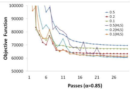
Figure 1: Bakeoff 2005 Chinese word segmenta-tion task: Objective funcsegmenta-tion with fixedα.
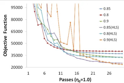
Figure 2: Bakeoff 2005 Chinese word segmenta-tion task: Objective funcsegmenta-tion with fixedη0.
rate parameter.
For our method, we first measured the progress of the SGD algorithm with heuristic line search we presented against the origin SGD method. We use the same parameters settings with the for-mer method including both regularization param-eter and learning rate paramparam-eters. The number of passes performed over the training data was also set to 30. Then we compare the results of both methods during the training process of the model with the same parameters, and they were shown in Figure 1 and Figure 2.
Figure 1 shows how the value of the objective function changed as the training proceeded with the same descent learning rate parameter (α = 0.85), the figure contains six curves
represent-ing the results of SGD method with heuristic line search and the origin SGD method with differ-ent initiation learning rate parameter settings (η0).
Table 2: Bakeoff 2005 Chinese word segmentation task. Accuracy of the model on the testdata.
L+R # Features F score
OWL-QN 56451.8 114,942 94.81
SGD 61398.6 232,585 94.92
Ours 56481.9 117,374 94.78
Table 3: Bakeoff 2005 Chinese word segmentation task. Training time of the model on the testdata.
Passes Time
OWL-QN 141 2h59min
SGD 30 58min
Ours 5 + 88 2h06min
result than the origin SGD method when using the same learning rate parameter settings. Figure 2 shows the results with different settings of learn-ing rate parameters (fixedη0 = 1), and it
demon-strates the same trend as Figure 1.
Then we trained the models with the training data and evaluated the accuracy of the Chinese word segmenter on the test data. The number of passes performed over the training data in SGD was also set to 30. In our method, we set the SGD iteration times to 5. It is worth noting that we didn’t spend much time in tuning the value of this parameter. Based on a cursory view of the train-ing process, we found that it converge to a relative “good” result after the first 5 iteration. We used this value throughout all the experiments. Because we would take the OWL-QN method to guarantee the final convergence, and the SGD method with heuristic line search strategy is insensitive to the learning rate parameters, this value would not have a significant influence on the performance.
The results are shown in Table 2 and Table 3. In Table 2, the second column shows the final value of the objective function. The third column shows the number of active features in the final result-ing model. The fourth column shows the F score of the Chinese word segment results, which is the harmonic mean of precision P (percentage of out-put Chinese words that exactly match the golden standard Chinese words) and recall R (percentage of golden standard Chinese words that returned by our system). In Table 3, the second column shows the number of passes performed in the training, in our method, this value includes the the number of
Table 4: Feature templates for name entity recog-nition task.
(1)ci−2yi,ci−1yi,ciyi,ci+1yi,ci+2yi
(2)ci−1ciyi,cici+1yi
(3)yi−1yi
passes both in the first stage of SGD and the sec-ond stage of OWL-QN process. The third column shows the training time.
In the terms of accuracy, there was no signif-icant difference between all the models, the ori-gin SGD method yield the slightly better result, probably due to the model has larger features sets. This doesn’t contradict to our original purpose, for we have got a substantial improved result in both the final value of the objective function and the number of active features compared with the ori-gin SGD method, and to the same level as OWL-QN method. Notice the origin feature sets are over 6 millon, L1 regularization methods produced the models which are compact indeed. The official best result in the closed test achieved an F score of 95.00, and our result is quite close to that, ranked 4th of 23 official runs.
On the other hand, our method took about 30% less than the OWL-QN method in the training time. Our method only needs 88 passes over the whole training data in the second stage for convergence compared with 141 in the OWL-QN method, which shows a significant improvement in training time consuming, for we have used the first stage of SGD method to get a nearly optimal and stable result beforehand.
4.2 Name Entity Recognition
The second set of experiments used the name en-tity recognition corpus from the Fourth Interna-tional SIGHAN Bakeoff data sets (Jin and Chen, 2008), provided by Microsoft Research Asia. The training data consists of 23,182 sentences, 1,089,050 Chinese characters and the testing data consists of 4,636 sentences, 219,197 Chinese char-acters. We separated 1,000 sentences from the training data and use them as the heldout data. The training data is annotated with the “IOB” tags rep-resenting name entities including person, location and organization.
Table 5: Fourth SIGHAN Bakeoff name entity recognition task. Training time of the model on the testdata.
L+R Passes Time
OWL-QN 11247.1 219 5h26min
SGD 13993.3 30 1h08min
Ours 11245.5 5 + 122 3h10min
Table 6: Fourth SIGHAN Bakeoff name entity recognition task. Accuracy of the model on the testdata.
# Feat. LOC ORG PER
OWL-QN 34,579 89.94 82.61 90.65
SGD 113,005 89.39 82.75 90.78
Ours 36,709 90.05 82.25 90.49
training data for convenient. Again a richer label representation may yield a better performance.
The other experiment settings are the same with the experiment on Chinese word segmentation. The comparison results are shown in Table 5, Fig-ure 3 and FigFig-ure 4. The trend in the results is the same as that of the Chinese word segmenta-tion task. SGD method with heuristic line search strategy produced more stable and robust result than the origin SGD method. Although there will have fluctuations sometimes (in Figure 4), the line search strategy shows the ability to find an appre-ciate step size in that case. Again our method con-verged to a much better solution against SGD in both the final value of the objective function and number of active features, and took about 40% less training time than OWL-QN.
The accuracy of the results is shown in Table 6, there was no significant difference between all the models as well. The F score of organization name entity recognition was worse than the results in person and location name entity, for organiza-tion name entities in Chinese often have a relative long distance dependency, which is not easy to be captured by our local feature templates in the Chi-nese character level.
5 Conclusion
We have presented a two-stage algorithm that can efficiently train L1-regularized CRFs. Experi-ments on two NLP tasks demonstrated that our method is effective and efficient by utilizing both
Figure 3: Fourth SIGHAN Bakeoff name entity recognition task: Objective function with fixedα.
Figure 4: Fourth SIGHAN Bakeoff name entity recognition task: Objective function with fixedη0.
the advantages of SGD and OWL-QN.
In the future, we intend to study how to use the results of the first stage of SGD learning to estimate the Hessian information, which can be provided for the second stage of quasi-Newton method to enhance the effectiveness of training. Borders et al. (2009) looked into this problem in a similar way. It is also worthwhile to investi-gate whether other adaptive learning rate schedul-ing algorithms can result in fast trainschedul-ing with our method, as in (Vishwanathan et al., 2006; Huang et al., 2007).
Acknowledgments
References
Galen Andrew and Jianfeng Gao. 2007. Scalable train-ing of l1-regularized log-linear models. In Proceed-ings of the International Conference on Machine Learning, pages 33–40. Corvalis, Oregon, USA.
Antoine Bordes, L´eon Bottou, and Patrick Gallinari. 2009. SGD-QN: Careful quasi-Newton stochastic
gradient descent. InThe Journal of Machine
Learn-ing Research, 10: 1737–1754.
L´eon Bottou. 2007. Stochastic gradient descent (sgd) implementation. http://leon.bottou.org/projects/sgd.
Stephen Boyed and Lieven Vandenberghe. 2004.
Con-vex Optimiaztion. Cambridge University Press.
Michael Collins, Amir Globerson, Terry Koo, Xavier Carreras, and Peter L. Bartlett. 2008. Exponentiated gradient algorithms for conditional random fields
and max-margin markov networks. InThe Journal
of Machine Learning Research, 9: 1775–1822.
Christian Darken and John Moody. 1990. Note on learning rate schedules for stochastic optimization. In Proceedings of Advances in Neural Information Processing Systems 3, pages 832–838. Colorado, USA.
Tom Emerson. 2005. The second international
Chi-nese word segmentation bakeoff. In Proceedings
of Fourth SIGHAN Workshop on Chinese Language Processing. Korea.
Jenny Rose Finkel, Alex Kleeman, and Christopher D.Manning. 2008. Efficient, feature-based,
con-ditional random field parsing. In Proceedings of
the Annual Meeting of the Association for Computa-tional Linguistics, pages 959–967. Columbus, Ohio, USA.
Jianfeng Gao, Galen Andrew, Mark Johnson, and Kristina Toutanova. 2007. A comparative study of parameter estimation methods for statistical natural
language processing. InProceedings of the Annual
Meeting of the Association for Computational Lin-guistics, pages 824–831. Prague, Czech republic.
Changning Huang and Hai Zhao. 2007. Chinese word
segmentation: A decade review. InJournal of
Chi-nese Information Processing, 21(3): 8–19.
Han-Shen Huang, Yu-Ming Chang, and Chun-Nan Hsu. 2007. Training conditional random fields by periodic step size adaptation for large-scale text
min-ing. InProceedings of the IEEE International
Con-ference on Data Mining, pages 511–516. Omaha, Nebraska, USA.
Guangjin Jin and Xiao Chen. 2008. The fourth inter-national Chinese language processing bakeoff: Chi-nese word segmentation, named entity recognition
and Chinese pos tagging. In Proceedings of Sixth
SIGHAN Workshop on Chinese Language Process-ing. India.
Junichi Kazama and Junichi Tsujii. 2003. Evalua-tion and extension of maximum entropy models with
inequality constraints. In Proceedings of the
Con-ference on Empirical Methods in Natural Language Processing, pages 137–144.
John Lafferty, Andrew McCallum, and Fernando Pereira. 2001. Conditional random fields: prob-abilistic models for segmenting and labeling
se-quence data. In Proceedings of the International
Conference on Machine Learning, pages 282–289. Prague, Czech republic.
Thomas Lavergne, Olivier,Capp´e, and Franc¸ois Yvon.
2010. Practical very large scale CRFs. In
Pro-ceedings the Annual Meeting of the Association for Computational Linguistics, pages 504–513. Upp-sala, Sweden.
Dong C. Liu and Jorge Nocedal. 1989. On the limited memory BFGS method for large scale optimization.
Mathematical Programming, 45: 503–528.
Andrew Mccallum, Dayne Freitag, and Fernando Pereira. 2000. Maximum Entropy Markov Mod-els for Information Extraction and Segmentation. In
Proceedings of the International Conference on Ma-chine Learning, pages 591–598. California, USA.
Naoaki Okazaki. 2007. CRFsuite: A fast
im-plementation of conditional random fields (CRFs). http://www.chokkan.org/software/crfsuite/.
Fuchun Peng, and Andrew McCallum. 2004. Accurate Information Extraction from Research Papers
us-ing Conditional Random Fields. InProceedings of
the North American Chapter of the Association for Computational Linguistics, pages 329–336. Mas-sachusetts, USA.
Lawrence Rabiner. 1989. A Tutorial on
Hid-den Markov Models and Selected Applications in
Speech Recognition. In Proceedings of the IEEE,
77(2): 257–286.
Charles Sutton and Andrew McCallum. 2006. An introduction to conditional random fields for
rela-tional learning. Introduction to Statistical
Rela-tional Learning. The MIT Press.
Kristina Toutanova, Aria Haghighi, and Christopher Manning. 2005. Joint learning improves semantic
role labeling. InProceedings of the Annual
Meet-ing of the Association for Computational LMeet-inguis-
Linguis-tics, pages 589–596. Michigan, USA.
Yoshimasa Tsuruoka, Junichi Tsujii, and Sophia Ana-niadou. 2009. Stochastic gradient descent train-ing for l1-regularized log-linear models with
cumu-lative penalty. In Proceedings the Annual Meeting
of the Association for Computational Linguistics, pages 477–485. Suntec, Singapore.
Douglas Vail, John Lafferty, and Manuela Veloso. 2007. Feature Selection in Conditional Random
the IEEE/RSJ International Conference on Intelli-gent Robots and Systems, pages 3379–3384. Cali-fornia, USA.
S. V. N. Vishwanathan, Nicol N. Schraudolph, Mark W. Schmidt, and Kevin P. Murphy. 2006. Accelerated training of conditional random fields with stochastic
gradient methods. In Proceedings of the