Calibration Methods of Hull-White Model
S´ebastien Gurrieri1∗, Masaki Nakabayashi1§ and Tony Wong1¶
1Risk Management Department, Mizuho Securities Tokyo
Abstract
We describe several strategies for the calibration of one factor Hull-White model with con-stant or time-dependent mean reversion and volatility parameters to the interest rate vanillas. We propose an efficient approximation formula for the swaption implied volatility which enables us to estimate the mean reversion independently of the volatility. We give the closed-forms for exact pricing using explicit integrals of the model parameters and propose parametric forms for the mean reversion and volatility. We test their performance in terms of quality of fitting and stability w.r.t. market changes, and show that excellent fits can be obtained without suffering from instabilities. Furthermore, our calibration methods and parameter control techniques allow for an elegant interpretation of market moves, which we illustrate with an in-depth analysis of Lehman crisis in the fall of 2008.
Contents
1 Introduction 2
2 Model Dynamics and Closed Forms 4
1
Introduction
Market models, pioneered by [2], [9], have recently emerged as a market standard for the pricing of exotic interest rate products. In these models, the dynamics of observable market rates, such as Libor and swap rates, are directly specified. They are appealing to market practitioners largely due to the fact that they can be calibrated to market caplet and swaption volatilities as well as an initial yield curve. In spite of their increasing popularity, market models have one serious drawback. An accurate implementation can only be made through simulation, which is typically slow due to the large number of state variables (i.e. the discrete–tenored market rates) needed to be evolved through time, and the complicated drift terms associated with the underlying stochastic differential equations (SDEs). This can be a problem for path dependent payoffs which require a large number of simulated paths in order to obtain sufficiently accurate price and risk figures. The problem can be even more acute for products with an early exercise provision as simulation is not naturally suited for performing backward–in–time calculations needed to determine the optimal exercise strategy.
In contrast to market models, affine term structure models (ATSMs) attempt to model the unobservable short rate, assumed to be an affine function of some latent factors. ATSMs have a few appealing properties. First, they are analytically tractable. In particular, closed–form solu-tions for caps/floors and efficient price approximation methods for European swapsolu-tions are often available. Second, Monte Carlo implementation of ATSMs is relatively straightforward compared to market models. In low dimensional cases, path–independent products with an early exercise provision can also be evaluated efficiently using lattice methods. Third, under ATSMs, all kinds of interest rates (e.g. forward Libor and swap rates with any expiry/maturity/payment dates) can be computed readily from the short rate factors, whereas in market models interpolation and extrap-olation are often needed when the product dates do not align with the canonical model dates. The computational efficiency offered by ATSMs explains why many banks still use these models for risk calculation and other risk management purposes even after the introduction of the market models. The main objective of this paper is to analyze in details the issues of model calibration and parameter control associated with a popular ATSM, known as one–factor Hull White (HW1F) model ([5], see [3] for a review). The HW1F model, which is characterized by a mean reversion and a volatility parameter, has been and is still very popular among market practitioners because of its parsimony and analytical tractability (thanks to the normality of the short rate). In spite of its popularity, the existing studies on the model calibration, especially in the case of time-dependent parameters, are rather scarce. In [6] and [7], the authors have covered the basic procedures for calibrating the HW1F model utilizing tree methods. However, there does remain several open issues related to its practical use.
In this work, we address the issues mentioned in the previous paragraph. This study provides an explicit realization of some ideas developed in [6] and [7] and supplements them with a thorough analysis of various issues involved such as parameter stability and relationship between model parameters and market prices of calibrating instruments. Hence, our work can be considered as a complement and a detailed follow-up for [6] and [7].
We introduce parametric forms for the time-dependent parameters, with additional constraints. These give us control over the parameters while still allowing enough fitting freedom. We de-scribe several calibration strategies, namely local and global, with constant and/or time-dependent parameters, with separate or simultaneous optimizations. We propose an approximation of the swaption implied volatilities, which, in the particular case of constant mean reversion and volatil-ity, leads to a very efficient (quasi-instantaneous) calibration method. This approximation, due to its simplicity and explicit form, provides further insights into the market/model relationships. The case of Lehman shock in the fall of 2008 and its consequences on the parameters are analysed in details. We emphasize the importance of the mean reversion parameter when attempting to fit over several different tenors, possibly over the whole swaption matrix. We finally conclude that, contrary to common beliefs, excellent fits to the whole swaption matrix can be obtained without traces of instabilities, when both the mean reversion and volatility are time-dependent.
2
Model Dynamics and Closed Forms
Hull-White model definition and properties are well-known and therefore we recall them only briefly here. Our main purpose is instead to provide the notations used in the closed-form calculations with the view to calibrating the model to vanilla options. More precisely, we want to display the variance of a zero-coupon bond ratio and the expressions of the functions characterizing the affine structure of the bond, in order to price swaptions analytically.
The closed-forms can be written thanks to various integrals of the mean reversion and volatility that can be found in [4]. We recall them in appendix A and write them slightly more explicitly, together with additional properties. We keep them under a symbolic form as long as possible such that the formulae remain valid for any specific parametric form that the user may choose. Note that they become explicit as soon as the mean reversion and volatility parametric expressions are specified. In particular, when these are constant, the integrals reduce to their standard form, given for instance in [3].
2.1 Dynamics
In the risk neutral measure, denoted byQ, the Hull-White short-rate SDE reads
dr(t) =
(
θ(t)−a(t)r(t)
)
dt+σ(t)dWQ(t), (1)
with the time-dependent functions a(t) for the mean reversion and σ(t) for the volatility. Exact replication of the initial curve is realized by fixing the functionθ(t) to the expression (39) given in appendix A.r(t) has a normal distribution with mean and variance
E
The zero-coupon bond P(t, T) has the affine structure
P(t, T) = exp
with integrated variance
Equation (8) holds due to property (34).
2.2 Closed Forms for Caplets and Swaptions
Caplets
Let us consider a caplet with strikeK, fixing timeTF and paying timeTP. This can be rewritten as a zero-bond put option (ZBP), priced by Black Formula with the variance of the bond ratio in (8), i.e.
Let us consider a (payer) swaption with strike K, maturityT0, swap tenorTP, and swap cash-flow times {Ti}i=1..n, with Tn =TP. This can be rewritten as a weighed sum of zero-bond (put) options using Jamshidian’s decomposition [8]. More precisely,
PSwaption(K, T0, TP) =
2.3 An Approximation of the Swaption Implied Volatility
direct relation between the market implied volatility and the model parameters. In this section, we suggest an approximation satisfying this goal.
From the definition of swaptions it is clear that if we could calculate the variance of a swap rate having a log-normal distribution (i.e. the SMM model), we would be able to calibrate simply by equating this variance with that obtained from the market implied volatility. Unfortunately, Hull-White model is not a swap rate model, the swap rate is not log-normal. However the bond ratio P(t,TF)
P(t,TP) is. This observation directs us toward an approximation relating the swap rate to
the bond ratio above. We follow the strategy proposed in [3] for BGM model and adapt it to the Hull-White case.
The approximation consists in assuming it is log-normal under the annuity measureA and try to calculate its variance, the quantity we need for pricing. To this end, we approximate the true swap rate S(t, T0, Tn) by ˜S(t, T0, Tn) with
Now applying Ito’s Lemma to the approximated swap rate above, we find
dS˜(t, T0, Tn) and changed measure from the Tn-forward to the annuity measure A. This introduces a drift but for pricing purpose we are only interested in the variance, which reads
Vswap(T0, Tn) =
intend to use it only to estimate the mean reversion, and later correct this estimation by a fitting to the actual analytical price.
Finally, note that due to the specific form ofVp(0, T0, Tn) in (8), the Hull-White implied variance
Vswap(T0, Tn) depends on the model volatility σ(t) only through the function Vr(0, T0), in other words the dependences in the swap tenor Tn and σ(t) are decoupled. This means that the ratio of two implied volatilities having the same maturityT0 is independent of σ(t), a feature that will enable us to estimate the mean reversion without knowledge of the volatility.
2.4 Parameter Specifications
One way to achieve at the same time ease of implementation and ability to integrate the functions
a(t) andσ(t) analytically is to set these to piecewise constant functions. This is what we will always do from now on, constant aand σ being just particular cases.
Let us call the parameter time grid {ti}i=0..N−1 where N is the number of points on the grid.
Let us illustrate this by assuming the time grid runs up to 30 years with 6M intervals. There are thenN = 61 points in the grid (t0 = 0,t60= 30). A generic piecewise constant function would thus be defined by 61 values, which means 122 parameters including the mean reversion and the volatility. This is clearly too much, so one must constrain them in some manner.
One natural way to reduce the number of parameters is to match their number with the number of market maturities, with the view to calibrating using a bootstrap-like method. If the first market maturity is att2 = 1, then one will enforce the conditions a1 =a0 and σ1 =σ0, and so on and so forth for the remaining maturities. Although this strategy is commonly used, probably due to its intuitive meaning and ease of implementation, we are not interested in developing it further here. It suffers from serious drawbacks, among which big jumps in values from one time to the other, causing instabilities, especially visible when pricing exotics.
We choose instead to constrain the parameters ai and σi to be generated by functional forms. The resulting number of free parameters will be that of the functional forms, while a suitable choice of such functional form will ensure that the functionsa(t) andσ(t) do not suffer from dangerously jumping values.
Apart from the constant case, in this work we will make use of the logistic function to generate the mean reversion, i.e. we define
ai = A0+
A1−A0
1 +eA2(A3−ti) (24)
whereA0..A3 are 4 parameters describing (heuristically)
• A2: the slope at the transition • A3: the time at the transition.
We call transition the area where the function changes rapidly between its early time and late time regimes. See fig. 1 for a visual example of the type of shapes it produces.
Figure 1: Piecewise constant mean reversion based on the logistic function Logistic[−5%,5%,0.5,10]
For the volatility we will study a functional form based on interpolating at the times{ti}i=0..N−1 a given grid of volatility vs. time {T˜k,Σk}k=0..N˜−1, i.e.
σi= CubicSpline(ti,{T˜k},{Σk}) (25)
where we interpolate with the Cubic Spline with left constraint of vanishing 2nd derivative and right constraint of vanishing 1st derivative. The volatilityσ(t) is set to constant after the last time
˜
3
Calibration Strategies
In this section we describe a few possible strategies for the calibration of Hull-White model to the market of swaptions. By calibration strategy we mean the following points:
1. The choice of constant or time-dependent mean reversion and volatility
2. The choice of products to calibrate to, and whether to calibrate locally or globally
3. Whether to optimize on the mean reversiona(t) and the volatilityσ(t) together or separately, and in the latter case, how to estimate one independently of the other.
3.1 Relations Market/Model parameters
Before diving into the calibration procedures, it is useful to investigate what types of swaption implied volatilities can be obtained from Hull-White model. Indeed the range of accessible volatil-ities is restricted, as it is not a market model such as LMM or SMM for which the market implied volatilities are inputs. On the contrary Hull-White model constrains the shape of the implied volatility matrix, and our goal in this section is to study the influence of the mean reversion and the volatility on this matrix.
First of all, we take a fixed constant mean reversion (1%) and change the value of the constant volatilityσ. We display the result in fig. 2, for the two maturities 6M and 10Y.
Figure 2: Implied Volatilities for model swaptions with different volatilities. Maturities 6M and 10Y, mean reversion a= 1%.
Apart from the intuitive fact that the implied volatility increases when the model volatility increases, we can observe that, at fixed maturity, the ratios between two implied volatilities with neighbouring tenors do not vary much with σ. This is an encouraging fact when considering the use of SMM approximation and will be discussed in more details in section 4.1. It means that σ
Note also that the level of the implied volatility decreases significantly when the mean reversiona
increases.
Figure 3: Implied Volatilities for model swaptions with different mean reversions. Maturities 6M and 10Y, volatility σ = 0.6%.
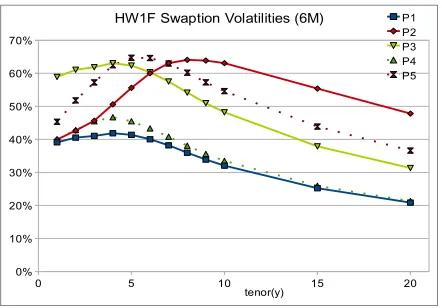
Figure 4: Implied Volatilities for model swaptions with different time-dependent mean reversions. Maturity 6M, model parameters
P1: σ = 0.2%a= Logistic[−30%,5%,1,3], P2: σ = 0.2%a= Logistic[−30%,5%,1,6] P3: σ = 0.3%a= Logistic[−30%,5%,1,3], P4: σ = 0.2%a= Logistic[−30%,5%,10,3] P5: σ = 0.2%a= Logistic[−50%,5%,1,3], P6: σ = 0.1%a= Logistic[−50%,5%,1,3]
All curves in fig. 4 are obtained from one another by changing the value of one of the parameters
σ and Ai, i = 0..3. Comparing curves P1 and P2 shows that we can control the position of the hump in time with parameterA3. Note however that since this makes the mean reversion negative on a longer range, the overall level of curve P2 has increased. This effect may be compensated by a decrease inσ.
Curves P1 and P3 provide an other example that increasing only the volatility gives a propor-tional level change.
Curves P1 and P4 show that one can control, to some limited extent though, the steepness of the hump by changing the parameter A2.
Curves P1, P5 and P6 show how to obtain a hump with bigger amplitude by taking more negative values for the mean reversion at early times (P5) and reduce the implied volatility level by decreasing the volatility.
From these examples we can see that a rather wide range of humped shapes can be obtained by suitably setting the values of the parameters of the logistic functionAi,i= 0..3, while compensating with the volatility σ to adjust the level.
Overall this tells us that the mean reversion and volatility must be considered as a set, each of them having a different impact on the implied volatilities. Moreover, both of them influence the level of these volatilities, a fact that should be kept in mind when trying to build an intuition of what values these parameters can take and how they vary in day-to-day market changes. For instance, the same volatility σ can be considered as big or small, depending on the value of the corresponding mean reversion.
3.2 Optimizing on the Mean Reversion or not
has a strong influence on rate correlations, see eq. (46), and therefore on exotics such as Bermudan swaptions. This was demonstrated in [4], and we also briefly address this last issue in section 4.7.
On the other hand, the second method attempts to calibrate both the mean reversion and the volatility parameters to a series of cap/floorlets and/or swaptions with different maturities and tenors. This is based on the fact that both model parameters have crucial impacts on cap/floorlets and swaption prices, as is evident from the numerical examples given in the previous section. An intuitive way to see this is that both the mean reversion and the model volatility parameterize the associated Heath–Jarrow–Morton (HJM) volatility function.
In the current work, we focus mainly on the second calibration method. However, we shall emphasize that the objective of this study is not to reach a conclusion as to which strategy is superior to the other. Our intention is rather to lay out the methodology and gather some concrete numerical results, which we believe is valuable from a practical point of view as such results are scarce in the existing literature.
For the sake of completeness and in order to have a frame of reference, we have also included in our analysis some numerical examples of the first calibration method described above1.
3.3 Bootstrap vs. Overall Calibration
The first strategy that comes to mind is of bootstrap type, i.e. to use the model parameters ai and σi from 0 to the first market maturity T1 to fit to the first instrument, and then the model parameters fromT1 toT2 to fit the second instrument at maturityT2, and so on and so forth.
Although the above method may feel natural, produce perfect fit for (at least some of) the chosen instruments, and has the advantage of requiring only low-dimension optimizations, it often results in big jumps in the parameters and tends to exhibit a high dependency on the initial values fed to the optimization algorithm. We consider these issues as serious drawbacks and prefer adopting the following strategy.
We give up the intention of exact-fitting some specific instruments, and consider them instead as a pool on which to optimize. We also choose parametric forms for the mean reversion and volatility, as explained in the previous section, with a number of model parameters and fitted instruments not necessarily equal. We then optimize on all model parameters to fit all the chosen market instruments at once, with a predefined distance (here L2) between the model and market prices, together with weights to focus on some instruments more than others.
The parametric forms actually put constraints on all parameters as a whole, such that if we choose the functionals suitably, no big jumps will appear. The drawback of this is that there is no more direct relation between parameters and instruments, and in general we need to perform multi-dimensional optimizations, which are more difficult to handle than one-multi-dimensional algorithms. It is one of the purposes of this document to prove that these methods are feasible and can produce more stable and meaningful results.
3.4 Calibration to Swaptions
Here we present three ways of proceeding, independently of whether the parameters are constant or time-dependent. The main difference between these methods is the treatment of the mean reversion. In the first method, we fix it. In the second method, we estimate it independently of the volatility, and then find the volatility. In the third method, we optimize on the mean reversion and the volatility simultaneously. All multi-dimensional optimizations are performed using a version of
1
the Simulated Annealing algorithm, see appendix B. Below are more detailed descriptions of these three calibration methods.
3.4.1 Method 1
In this calibration method we do not optimize on the mean reversion, which is fixed to some arbitrary (constant) value to be specified by the user. We therefore optimize on the volatility only, such that the analytical price PVmod
a (Mi, Tj)(σ) approaches the market price PVmkt(Mi, Tj). PVmod is the price of a swaption as calculated in eq. (12), at ATM, and the subscripta indicates that the mean reversion has been fixed previously. In other words, our calibrated volatility is the point σ (possibly multi-dimensional) at which the function
Ga(σ) =
has its minimum. The initial point of the optimization must be chosen by the user. For the time-dependent case, one can first optimize for a constantσ and use the result as a hint for the initial point of the multi-dimensional optimization, in order to improve the speed of convergence. Wi,j are the user-defined weights.
3.4.2 Method 2
The second method is divided into two steps:
1. Estimate the mean reversiona(t) using SMM approximation for the implied volatilities
2. Optimize on the volatility using the exact analytical price, knowing the mean reversion from step 1).
Step 1) above is rendered possible, without knowledge of the volatility, thanks to property (8) of SMM approximated implied volatilities. Indeed, taking the ratio of two implied variances with the same maturityMi but different tenors Tj and Tk, we find, This means that by optimizing such that ratios of the type (27) approach their market counter-part, one can obtain an estimation of the mean reversion without knowing the volatility function
σ(t). More precisely, let us denote by IVi,j the market implied volatility for the swaption of ma-turity Mi and tenor Tj, with nm maturities and nt tenors. Our calibrated mean reversion is the point a(possibly multi-dimensional) at which the function
has its minimum. In case a weight Wi,j = 0 is met, it is simply ignored in the sum as we do not intend to use the corresponding swaption for calibration. The index j will then be chosen as the next one such thatWi,j 6= 0.
Step 2) is an optimization on the volatility σ(t) such that the analytical price approaches its market counterpart. In other words, our calibrated volatility is the point σ (possibly multi-dimensional) at which the function defined in (26) has its minimum, with the mean reversion fixed at step 1).
3.4.3 Method 3
The third method is conceptually more simple and goes into one step only: optimize on the mean re-versionandthe volatility such that the analytical price approaches the market price. In other words, our calibrated mean reversion and volatility are the pointsaand σ (possibly multi-dimensional) at which the function
G(a, σ) = ∑ 1≤i≤nm,1≤j≤nt−1
Wi,j
(PVmod(M
i, Tj)(a, σ) PVmkt(M
i, Tj) − 1
)2
(29)
4
Numerical Results
In this section we display numerical results of calibrations to JPY ATM swaptions using the various methods described in Section 3. Similar strategies can be applied to other currencies. We show examples of calibration to USD and EUR swaption markets in Appendix C.3 and C.4.
4.1 Performance of SMM approximation
The SMM approximation formula (19) has shed some light on the roles of the mean reversion and volatility parameters in determining implied swaption volatilities. In this section, we attempt to verify the implication of the SMM approximation formula and its accuracy through some numerical examples.
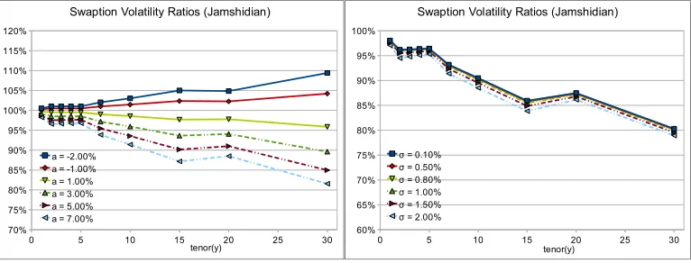
In the left panel of Figure 5 below, we display the ratios of the implied volatilities of swaptions with a 5–year maturity and adjacent tenors under various mean reversion parameters. Here, we fix the volatility parameter to 0.5%. The right panel focuses on the impacts of changing the volatility parameters on the implied volatility ratios with the mean reversion fixed to 8%. All implied volatilities used in Figure 5 are computed using the Jamshidian decomposition method. It is clear that the implied volatility ratio curve moves systematically downward as the mean reversion parameter increases. In contrast, the changes in implied volatility ratios are relatively insignificant as the volatility parameter varies. This observation indeed agrees with what the SMM approximation formula suggests: implied volatility ratios of swaptions with the same maturity date depend mainly on the mean reversion parameter. It is this observation that motivates the introduction of the second calibration strategy described in the previous section in which the mean reversion and volatility parameters can be calibrated separately.
Figure 5: Swaption Implied Volatility Ratios, maturity 5Y. Left: changing aat fixedσ
Right: changingσ at fixeda.
the maturity of the swaptions to 5 years while changing the underlying swap tenors from 1 year to 30 years. From these figures, we see that the SMM approximations appear to be able to capture the qualitative behavior of the benchmark swaption implied volatilities obtained from the Jamshidian method. However, under certain cases, the approximated swaption implied volatilities are quite far from the benchmark values calculated from the Jamshidian method. For example, in the third panel, the discrepancies between the SMM approximated volatilities and the benchmark values can be more than 10% for swaptions with long tenors. Indeed, we have run the same comparison tests under many other parameter values and the results agree what we have suggested before: the SMM approximation can be crude and is not meant to be used for actual pricing purposes.
We emphasize that the SMM approximation shall be used as a means to understand the qual-itative behavior of the implied swaption volatilities in terms of the HW model parameters, which can be useful from model control point of view. Its accuracy can vary very much depending on the model parameter values and the tenor and maturity of the underlying swaption. Hence, it cannot serve as a reliable way for pricing swaptions in general. In this next section, we shall also demon-strate numerically the effectiveness of the calibration demon-strategy utilizing the SMM approximation result.
4.2 Choice of Instruments
As an illustration consider the case of a calibration to JPY swaptions, for which we have 10 maturities and 12 tenors, in other words 120 swaptions. That is not to say there are 120 degrees of freedom (d.o.f.). As it is not clear what the actual number of d.o.f. is, we do not know exactly how many parameters in the model can be used to fit how many swaptions. This requires testing. In the tests we present here, we will consider 3 instrument choice scenarios. The first one represents a strategy commonly used, the local calibration, in parts for hedging reasons, which consists in picking swaptions with fixed co-terminal (maturity + tenor). We will consider here the 20Y co-terminal calibration. In practice this means that we choose non-zero weights Wi,j only for one swaption per maturity.
The second scenario is an extension of the previous one where we consider 2 co-terminal dates, 10Y and 20Y. The purpose of this test is to analyse the behaviour of the calibration procedure when we increase the quantity of information and see how this translates in terms of model parameters. This is rather a toy strategy, we are not aware of its actual use in the industry.
Finally the third scenario represents the calibration to the whole swaption matrix, i.e. global calibration. The goal here is to take into account all the market information and analyse, on the one hand how many model parameters are needed to describe it and on the other hand what is the best fitting quality that we can hope for, knowing that perfect fit to the whole matrix cannot be expected in this model.
We will consider a testing period of 2 years between Nov. 2007 and Sept. 2009 where we will perform the calibration weekly.
4.3 Co-terminal 20Y
According to our interpretation of the mean reversion as influencing strongly the slope of the swaption implied volatility curves, in the tenor direction, it seems risky to calibrate it in the settings described here. Indeed, the only information we have is 1 number for each maturity, such that we have no information at all on the slope.
over our testing period. It bears big jumps from weeks to weeks such that even its overall order of magnitude is unclear. Although it is not obvious what this order of magnitude should be, such jumps do not seem acceptable for pricing in practice. We will therefore conclude that it is too unstable to optimize on the mean reversion when only 1 instrument per maturity is chosen, such that in the remainder of this subsection, we keep the mean reversion fixed over the testing period. Now we fix the mean reversion at the value obtained on Nov. 27th, 2007 with Method 3, i.e.
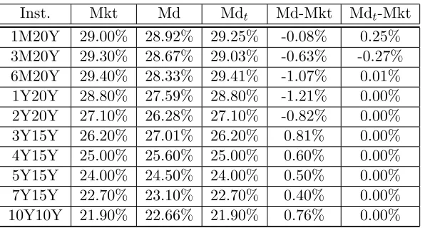
a= 0.97%, and proceed to calibrating the volatility as a constant or time-dependent function. We are interested in 2 aspects, the stability of the parameters over the 2 year period of our tests, and the quality of the fit to the considered market instruments. For the volatility functionσ(t) we first consider a 10pts function with no constraints on the parameters, such that, having the same number of parameters as fitted instruments, we can hope for a perfect fit. This is indeed what happens, as can be seen in table 1 below, which gives an example of fit quality comparison between the constant and time-dependent calibrations. ”Mkt” refers to the market implied volatilities, ”Md” to the model implied volatilities for constant σ, and ”Mdt” to the model implied volatilities for time-dependentσ(t).
Table 1: 20Y Fitted JPY swaptions on 2009/09/08, no parameter constraints
Inst. Mkt Md Mdt Md-Mkt Mdt-Mkt
Apart from the earliest maturities, which are not very liquid anyway, the fit is nearly perfect in the case of the time-dependent model volatility. However a study of the stability of the parameters over the testing period shows in fig. 25 in the appendix that, while the constant volatilityσand the parameter Σ0of σ(t) are stable, the parameter Σ9 ofσ(t) is very noisy. We conclude that although we can reach a nearly perfect fit for most chosen instruments, there is again over-fitting, this time due to σ(t).
Figure 6: Volatility calibrated to 20Y co-terminal at fixed mean reversion. Constraint α= 0.1. Left: constant σ, parameters Σ0 and Σ9 of σ(t)
Right: objective function for constant σ and time-dependentσ(t).
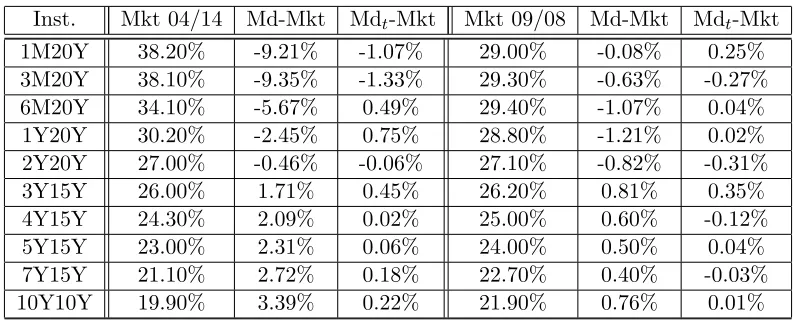
Once the constraint has been enforced, the calibration result becomes stable. As should be expected, the time-dependence of the volatility always improves the quality of the fit, though this improvement may be more or less significant depending on the dates. It appears to be particularly efficient in times of unstable or quickly changing markets, for instance at and after Lehman crisis at the fall of 2008.
In terms of quality of fitting to the chosen instruments, we display in table 2 the result of the calibration on the dates 2009/04/14 and 2009/09/08. As can be seen in fig. 6, 2009/04/14 is typical of the ”after-Lehman-shock” period, extending over several months, during which calibration with constant parameters behaves relatively poorly.
Table 2: 20Y Fitted JPY swaptions in 2009,α= 0.1
Inst. Mkt 04/14 Md-Mkt Mdt-Mkt Mkt 09/08 Md-Mkt Mdt-Mkt
1M20Y 38.20% -9.21% -1.07% 29.00% -0.08% 0.25%
3M20Y 38.10% -9.35% -1.33% 29.30% -0.63% -0.27%
6M20Y 34.10% -5.67% 0.49% 29.40% -1.07% 0.04%
1Y20Y 30.20% -2.45% 0.75% 28.80% -1.21% 0.02%
2Y20Y 27.00% -0.46% -0.06% 27.10% -0.82% -0.31%
3Y15Y 26.00% 1.71% 0.45% 26.20% 0.81% 0.35%
4Y15Y 24.30% 2.09% 0.02% 25.00% 0.60% -0.12%
5Y15Y 23.00% 2.31% 0.06% 24.00% 0.50% 0.04%
7Y15Y 21.10% 2.72% 0.18% 22.70% 0.40% -0.03%
10Y10Y 19.90% 3.39% 0.22% 21.90% 0.76% 0.01%
4.3.1 Conclusion
We conclude from these tests that the time-dependency of the volatility enables us to adapt in a more flexible way to different types of swaption matrices that may appear in times of large market moves. Some quality of fitting has been lost compared to the unconstrained volatility case, but stability has greatly improved.
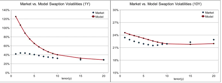
Although we have chosen a specific set of instruments and analysed the fitting quality for these instruments, it is interesting to have a look at how the other swaptions were fit. In fig. 7, we display the market and model swaptions at the 1Y and 10Y maturities, for the time-dependent volatility with constraint calibration scheme. We can see that away from the chosen instruments, the model swaptions can be off by a very large amount, especially for early maturities and in the presence of a hump.
Figure 7: Market and Model Implied Volatilities on 2009/09/08, constanta, time-dependentσ(t) Left: maturity 1Y, calibrated instrument at tenor 20Y
Right: maturity 10Y, calibrated instrument at tenor 10Y
4.4 Co-terminals 10Y and 20Y
4.4.1 Constant a and σ
Here we compare the results of the 3 methods described in section 3.4. We briefly summarize them below.
• Method 1The mean reversion is fixed and the volatility is calibrated by using the analytical prices. This means we perform one 1-dimensional minimization.
• Method 2 The mean reversion is calibrated separately by using the approximated implied volatility ratios, while the volatility is calibrated by using the analytical prices. This means we perform two 1-dimensional minimizations successively.
• Method 3 The mean reversion and volatility are calibrated simultaneously by using the analytical prices. This means we perform one 2-dimensional minimization.
Figure 8: Constanta andσ are calibrated to the co-terminals 10Y and 20Y.
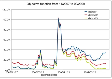
We observe that all these methods have a similar satisfactory stability. On top of this, we see a clear regime change in the mean reversion at the time of Lehman crisis. After this, the mean reversion is clearly lower than before. This echoes a structural change in the swaption matrix that will be discussed in more details in section 4.6.
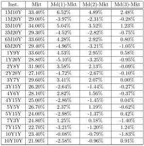
As to the quality of the fit to the chosen swaptions, we find the target values in fig. 9 for all dates and the detailed fitting errors in table 3 for the particular date 2009/09/08.
Table 3: 10Y and 20Y co-terminal fitted JPY swaptions on 2009/09/08
Several conclusions can be drawn from these numbers. Up to the Lehman crisis time, Method 1 and Method 3 behave quite similarly. This is natural as the fixed mean reversion is the calibrated one on the first day, and the mean reversion with Method 3 does not vary much during this period, such that its original value on 2007/11/27 remains a good estimation. However from the time the crisis is triggered, we have seen that the mean reversion enters a new regime. Method 1 is then no longer able to adapt to the new market conditions. Method 2 on the other hand, while fitting not as well as Method 3 since it is not a true 2-dimensional optimization, is nevertheless able to take into account the new situation after the shock.
We conclude that the mean reversion can be estimated safely when two co-terminal swaption information is included, and that it should be optimized on if one wants to adapt to changing market conditions. While method 3 is a true 2-dimensional optimization and therefore offers the best fitting quality in these parameter settings, it is clearly slower at runtime. Method 2 represents an alternative for which we can both adapt to market changes and have a very short runtime (quasi-instantaneous), if one is ready to sacrifice a little fitting quality.
4.4.2 Constant a and Time-Dependent σ(t)
Similarly to the constant σ case, we can distinguish the 3 methods
• Method 1: the mean reversion is fixed, and we perform one multi-dimensional optimization on the parameters Σk of σ(t)
• Method 3: the mean reversion and the volatility are calibrated simultaneously in one multi-dimensional optimization onaand the parameters Σk of σ(t).
First of all, let us compare the constant and time-dependent volatility calibrations. In fig. 10 we display the targets over the test period. In order not to burden the text with too many graphics, we show only the result for Method 3, similar conclusions holding for the other methods.
Figure 10: Calibration to co-terminals 10Y and 20Y, constant a, Method 3.
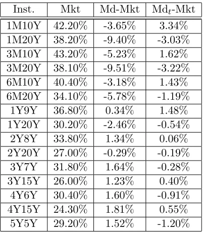
As can be expected, time-dependence represents a clear improvement in general, though for some special dates it might be less significant. Indeed, it may happen that the global minimum of the target function is obtained for an almost constant σ(t). Such situations occur in the summer of 2009, as can be seen in the figure above. Outside of these periods, the improvement due to time-dependence is obvious. We display the detailed fitting results for such a case in table 4.
Table 4: 10Y and 20Y fitted JPY swaptions on 2009/04/14,α= 0.1
Inst. Mkt Md-Mkt Mdt-Mkt
1M10Y 42.20% -3.65% 3.34%
1M20Y 38.20% -9.40% -3.03%
3M10Y 43.20% -5.23% 1.62%
3M20Y 38.10% -9.51% -3.22%
6M10Y 40.40% -3.18% 1.43%
6M20Y 34.10% -5.78% -1.19%
1Y9Y 36.80% 0.34% 1.48%
1Y20Y 30.20% -2.46% -0.54%
2Y8Y 33.80% 1.34% 0.06%
2Y20Y 27.00% -0.29% -0.19%
3Y7Y 31.80% 1.64% -0.28%
3Y15Y 26.00% 1.23% 0.40%
4Y6Y 30.40% 1.60% -0.91%
4Y15Y 24.30% 1.81% 0.55%
Inst. Mkt Md-Mkt Mdt-Mkt
5Y15Y 23.00% 2.22% 0.84%
7Y3Y 27.20% 1.22% -1.90%
7Y15Y 21.10% 2.97% 1.29%
10Y1Y 25.10% 0.74% -2.17%
10Y10Y 19.90% 3.39% 1.47%
Note also that now that we fit to a larger number of swaptions, a near-perfect fit can no longer be hoped for, considering the number of model parameters available here.
In fig. 11 we compare the fit to the co-terminals 10Y and 20Y for the 3 calibration methods described in this subsection, all with a time-dependent model volatility.
Figure 11: Calibration to co-terminals 10Y and 20Y, constantaand time-dependent σ(t)
We find that these targets reproduce a similar pattern as for the constant volatility case. Conse-quently the same conclusions hold, i.e. that calibrating the mean reversion is preferable, especially in case a wildly changing markets, and that simultaneous calibration performs better in terms of fitting quality than separate calibration of the mean reversion and volatility. For the particular date 2009/09/08, the detailed errors for each method are given in table 5 below.
Table 5: 10Y and 20Y co-terminal fitted JPY swaptions on 2009/09/08
Inst. Mkt Md(1)-Mkt Md(2)-Mkt Md(3)-Mkt
1M10Y 33.40% 5.14% 3.75% 1.76%
1M20Y 29.00% -5.11% -3.11% -0.89%
3M10Y 34.00% 3.73% 2.44% 0.55%
3M20Y 29.30% -5.62% -3.58% -1.33%
6M10Y 33.60% 4.38% 3.00% 1.02%
6M20Y 29.40% -5.18% -3.15% -0.91%
1Y9Y 33.60% 4.55% 3.05% 0.85%
1Y20Y 28.80% -5.40% -3.18% -0.77%
2Y8Y 31.90% 4.04% 2.45% 0.03%
Inst. Mkt Md(1)-Mkt Md(2)-Mkt Md(3)-Mkt
In terms of runtime, these 3 methods differ only by their treatment of the mean reversion. Since the volatility is time-dependent, in any case we must run a multi-dimensional constrained optimization, the question is whether to run it on 10 parameters (volatility only) or 11 (volatility and mean reversion). The runtime difference is not such that one can consider Method 2 as significantly faster than Method 3.
4.4.3 Time-Dependent a(t) and σ(t)
For both available methods (separate or simultaneous optimization), we find an unstable behaviour of the calibrated mean reversion parameters. We are now fitting to 2 co-terminals, that is, 20 swaptions, however not all the swaptions are independent d.o.f. Considering that we are using 10 + 4 model parameters, though constrained, it appears that we do not have enough information to fix their values in a stable way suitable for practical use. Furthermore even if we allow the calibration to run in this manner, we do not observe a drastic improvement due to the introduction of the time-dependent mean reversion. We conclude that the new d.o.f. coming from the mean reversion are superfluous when only 2 co-terminals are fitted and that it is safer to use a constant mean reversion.
4.4.4 Conclusion
A significant improvement in the fitting quality can be observed when including the mean reversion in the calibration procedure. Tests show that a constant mean reversion together with a time-dependent volatility can be obtained in a stable way while preserving a good quality of fit. It appears difficult and not particularly profitable to optimize on a time-dependent mean reversion. Simultaneous calibration of the constant mean reversion together with the volatility also brings a clear improvement of the fit while retaining stability.
While the 2 chosen co-terminals are approached with a reasonable accuracy by the model implied volatilities, we do not have any control on the rest of the swaption matrix. By focusing on 2 instruments per maturity, we may miss the other ones by quite a large amount, especially for early maturities, in a similar fashion to fig. 7. The hump in particular, is not captured at all.
4.5 All Instruments
Finally we consider the fit to all instruments in the swaption matrix.
of this in fig. 26 in the appendix. It may occur that only one instrument is fitted correctly, and the user would not be able to know in advance which one, which is quite a risky bet.
However, depending on the trade details and the purpose of the practitioner, it may be desirable to obtain a reasonable fit on the overall matrix. We have observed in the previous section that focusing on (a) particular co-terminal(s), even by optimizing on the mean reversion, has the disad-vantage that other instruments may be seriously mis-priced. On the other hand, trying to optimize on a time-dependent mean reversion resulted in an unstable behaviour, which we attributed to the lack of information to constrain the mean reversion parameters.
It is therefore natural to wonder whether the information contained in the whole swaption matrix is suitable to stabilize a time-dependent mean reversion, and if so, how good the resulting fit would be. In this section we attempt to answer these questions. As method 2 did not seem to yield a significant runtime or stability improvement in the case of the calibration to 10Y and 20Y co-terminals, we will consider here only method 3, i.e. simultaneous calibration of the mean reversion and volatility in one multi-dimensional optimization.
First of all, in fig. 12 we compare the calibration targets over 2 years for the 3 strategies constant
aand σ, constantaand time-dependentσ(t), and finally both time-dependent a(t) and σ(t).
Figure 12: All instruments are fitted.
We can see that the time-dependence of the mean reversion gives us a spectacular improvement in the fitting quality.
It also appears that by calibrating to the whole swaption matrix we are less sensitive to Lehman crisis as can be seen from the shapes of the curves in the figure above, where we can no longer see the target spikes observed when calibrating to the co-terminals only. Whether this is a good feature or not is a matter of opinion. Being able to fit in a satisfactory way even in times of crisis may seem desirable as it avoids the danger of mis-pricing (or mis-hedging). On the other hand, a trader may hope that the model will be able to signal unusual market conditions by producing unexpected numbers, such as a bad fit quality.
Figure 13: ParametersA0 andA1 for constraintα= 0.1
Figure 14: Parameters Σ0 and Σ9 for constraintα= 0.1
There does not seem to be any obvious instabilities. The behaviour of the parameters is similar to that observed for the constant calibrations, the mid/long-term mean reversion (A1) also showing the regime change after Lehman crisis.
Figure 15: Market and Model Swaptions on the 2007/11/27 forα= 0.1
Figure 16: Market and Model Swaptions on the 2009/09/08 forα= 0.1
The quality of fit is greatly improved compared to the constant mean reversion case, and we no longer wildly mis-price any of the instruments, while retaining the stability of the parameters.
Figure 17: Market and Model Swaptions on the 2007/11/27 forα= 0.5
We can see that thanks to the new freedom we could fit the swaption even more accurately. We obtain now an excellent fit to the whole matrix, including the hump, while the parameters have the following evolution over the two year testing period
Figure 19: Parameters Σ0 and Σ9 for constraintα= 0.5
Unsurprisingly, they seem to bear wider moves than for the stronger constraintα = 0.1, although how much stability has been lost remains ambiguous, as it is not clear how to measure it objectively. We do not see here evidence of over-fitting as can be observed in other calibration scenarios such as the unconstrained cubic spline or the calibration of a mean reversion to only one co-terminal, see fig. 24 and fig. 25.
4.5.1 Conclusion
There seems to be enough information in the swaption matrix to obtain a stable estimation of a time-dependent mean reversion together with a time-dependent volatility. The resulting fit can be excellent over the whole swaption matrix without evidence of over-fitting.
4.6 Model and Market Evolution: analysis at Lehman Crisis
Although a perfect mirroring of the market evolution in terms of model parameters cannot be hoped for, due to limitations of Hull-White model as mentioned in the introduction, we have observed during this 2 year testing period a clear change in the mean reversion, visible across all types of calibration and parameter control strategies. As this behaviour is unambiguously exhibited by the model and its calibration methods, we can be confident that it is more than just a numerical coincidence and bears instead a deep meaning.
Recall that at the time of Lehman crisis, at the fall of 2008, the mean reversion suddenly drops to lower values, and does not return to its pre-shock values (at least until the end of the testing period in fall 2009). This can be observed for example in fig. 8 for constant mean reversions, or on the mid/long-term parameter A1 of the time-dependent mean reversion in fig. 13. At the same time, the model volatility does not seem to react in a significant way, such that one can say that Lehman crisis has been essentially absorbed in a mean reversion regime change.
As this change is obvious on the model side, we would like to know what is its market counter-part. In other words, we are trying to figure out what is or what are the features of the swaption matrix and the yield curve that have drastically changed at and after Lehman shock, and why they affected the model parameters in such a way.
we believe it is possible to draw a few conclusions.
First of all, we would like to separate, if possible, the influence of the swaption matrix from that of the yield curve. To this end, we go back to the 10Y and 20Y co-terminals calibration, with constant mean reversion and volatility for simplicity. We again calibrate over the 2 year testing period, except that this time, we fix the swaption matrix to its value on the first day, and only change the yield curve. We obtain the calibration result in fig. 20, with the legend ”VC – FS”. Then we can fix the yield curve on the first day, and change only the swaption matrix. This result is displayed in fig. 20 under the legend ”FC – VS”. And finally, we can perform a ”real” calibration where both the curve and the swaptions vary. This has already been done and is represented in fig. 20 by the legend ”VC – VS”.
Figure 20: Difference in influence of the yieldcurve and the swaptions on the model parameters.
To sum up,
• VC – FS: the curve varies but the swaptions are fixed. Although there is a reaction of the parameters when Lehman crisis is triggered, this effect is not propagated afterwards and the parameters go back to similar values as before the shock.
• FC – VS: the curve is fixed but the swaptions varies. In this case we observe a behavior very similar to that of the real calibration, VC – VS, in that the mean reversion falls at the crisis and stays low afterwards.
• VC – VS: both the curve and the swaptions vary. This is the real calibration.
From all this we conclude that the regime change in the mean reversion has been caused mostly by the evolution of the swaption matrix2.
We display then the evolution of 4 different swaption implied volatilities (market) in fig. 21.
2
Figure 21: Evolution of JPY swaption implied volatilities
We observe two basic effects here. First of all, a level change appearing at the shock time and continuing afterwards. Second, a change in the relative values of the implied volatilities for the same maturity. This change is larger and most obvious for the 10Y swaptions, but is also visible at the 1Y maturity.
As we have discussed in section 4.1, fig. 5, a strong change in the ratios of implied volatilities at fixed maturity cannot be accounted for by a change in the model volatility, but rather in the mean reversion. Furthermore, since we observe in fig. 21 that the market implied volatilities have become flatter in the tenor direction, we deduce that this effect should be accounted for by a reduction of the value of the mean reversion, going possibly to negative values. This is indeed what is observed and what we have called a ”regime change”. It constitutes one more argument in favor of the consistency of the calibration methods proposed in this work.
4.7 Bermudan Swaptions
Finally we address an issue that we have not dealt with until now, i.e. the fixing of the mean reversion in the case of a local calibration to one co-terminal. As we have shown in section 4.3, it is not safe to optimize on it in this case. This means that the mean reversion has to be fixed by the user, leading to an ambiguity on its value. Moreover, the subsequently calibrated volatility will depend on the chosen mean reversion value, so one may wonder what can be the influence of this a priori ad hoc choice on products other than simple vanilla options.
Here we fix 3 different (constant) mean reversions and calibrate the time-dependent model volatility to the 10Y co-terminal over the 2 year testing period. As the volatility is time-dependent, we obtain very close fits to the European swaptions whatever the mean reversion is. For the 10Y Bermudan swaptions, we find the results in fig. 22.
As was also documented in [4], we observe a strong influence of the mean reversion on the Bermudan swaption prices, even though the relevant European swaptions are almost perfectly fit. This means that a trader can use this extra freedom to impose a view on the Bermudan swaptions. Alternatively, this can be viewed as an extension of the calibration process, in which Bermudan swaption information is also included.
Figure 22: 10Y Bermudan Swaption Prices (non-call 3Y) for mean reversions 6%, 0.5% and−3%.
reversion is preferable and therefore there is no more freedom in the model to impose a view on other products.
5
Conclusion
The achievements of this work are two-fold. On the one hand, we provided a detailed documentation and numerical examples about the calibration methods of Hull-White model with time-dependent parameters, as we believe this was missing from the literature. We hope that the readers will find it useful as a starting point to implement their own calibration and that it will spare them the trouble of tedious trials and errors.
On the other hand, we showed that some common negative opinions and fears about the model are not necessarily justified. It is widely stated, for instance, that Hull-White model cannot fit the swaption matrix well, and that introducing time-dependent parameters to improve the fitting quality results in unstable behaviours. We believe this work has proved this is not the case, provided a suitable calibration strategy is adopted. In particular, we showed that the fully time-dependent model can achieve excellent fit in a stable manner. Furthermore, we provided some means, such as the ”SMM” approximation of the implied volatilities, to interpret the behaviour of these parameters w.r.t. market moves. In particular, we showed that the model can provide interesting insights in the analysis of Lehman crisis in the fall of 2008.
It is not our purpose here to single out one best method. Instead we show that several calibration methods, such as local or global, with constant or time-dependent parameters, are acceptable, and that the choice depends on the user preferences as to fitting quality, runtime and ease of implementation. More specifically, it is clear that time-dependent parameters offer a better fitting quality, which comes at the cost of a slightly more complicated implementation of nested analytical integrals. We showed how to avoid the dangers of over-fitting, by using parametric forms with further constraints. However this method requires, in most cases, multi-dimensional constrained optimizations, representing an extra implementation and manipulation difficulty. In these tests we have used a customized version of the simulated annealing algorithm, which, while easily dealing with constraints, converges quickly enough for most practical purposes. In the particular case of a calibration with constant mean reversion and volatility though, the 2-dimensional optimization can be broken down to two 1-dimensional optimizations due to a property (approximate) of the model implied volatilities, captured by SMM approximation. For a user favoring ease of implementation and speed over fitting accuracy, a quasi-instantaneous method is thus available in which the mean reversion can be estimated. Note that this approximation may be made more accurate using the ideas of [1]. The generalization to time-dependent parameters, and its application to the calibration procedure, are currently under investigation in [10].
We believe that a number of open questions deserve further investigation in the future. First of all, the notion of instability of the parameters is quite ambiguous. In order to be able to run calibration in an automated way and discard the unstable methods, it would be useful to have an objective criterion as to what constitutes an unstable set of parameters.
Furthermore, the parametric forms proposed here are only suggestions and by no means the only possibilities. It may prove valuable to investigate the behaviour of other parametric forms, with different degrees of freedom. As we have briefly mentioned in the case of the local calibration, leaving the constant mean reversion undetermined by the calibration to European instruments may be desirable. The parametric forms and constrained multi-dimensional optimizations proposed here provide a suitable starting point to generalize this idea to more flexible calibration schemes in which the information of other products, such as Bermudan swaptions, may be incorporated.
understanding of the model implications and possibly discover other regime changes in the market.
Acknowledgments
We would like to thank T. Hayashi for providing us with convenient and efficient tools to access market data, and O. Lenoble for his remarks which helped improve the manuscript.
Appendix
A
Integrals
The basic integral that appears in most intermediate equations and final closed forms is based on integrating only the mean reversion. We denote it by E(t), and it has the expression
E(t) =eR0ta(u)du. (30)
From it we obtain the B(t, T) function involved in the affine structure of the discount bond
B(t, T) =E(t)
where 05s5tandf(0, t) is the initial instantaneous forward rate. The variance of the short-rate is given by
P(r(t)<0) =N(−√α(t)
Vr(0, t)
) (38)
whereN(x) is the normal cumulative distribution function.
For the functionθ(t) involved in the SDE (1) and ensuring exact replication of the initial curve, we find
Finally, other useful formulae include the expression of the instantaneous forward rate at t
f(t, T) =f(0, T) + E(t)
and the relation between the discount bound and the short-rate
B
Simulated Annealing
There are many different ways of running a simulated annealing algorithm, all centered on the same idea of drawing the next point randomly. Our version is based on the following steps
1. Choose an initial point x0 and set running variable xr=x0
2. Evaluate the function and record its value under variablefr=f(x0)
3. Draw a random pointx under a normal distribution of meanxr and standard deviationσj
4. Check ifx satisfies the constraints. If it does, go to step 5. If it does not, go back to step 3.
5. Evaluate f(x)
6. i) If f(x)< fr then the new point is closer to the minimum. It is thus recorded : fr =f(x) and xr=x.
ii) Iff(x)=fr then the new point does not represent an improvement. We can forget about it.3
7. Go to step 3 until stop condition is met. Minimum is atxr with function valuefr.
If we have some intuition of where the minimum is, we should take a small standard deviation
σj. The algorithm will then focus on the region around our initial estimate and thus converge faster. If however we have little information about where this minimum could be (and its unicity, and the existence of a global minimum and local minima, etc...), we should take a large σj, such that the algorithm will explore a large portion of the parameter space.
For the stop condition, we advise to perform a number of convergence tests to observe how many function evaluations are necessary to reach a satisfying degree of convergence and runtime. In pratice, for a 10-dimensional optimization, a few thousands of evaluations may be necessary, but runtime on a single 3.0GHz CPU typically does not exceed 10s.
Finally, we introduce a ”cooling down” mechanism realized by a decrease of the standard devi-ation σj with each iteration j, according to
σj =σ0∗exp(−γ× j
N−1) (49)
whereN is the total number of simulations,σ0 is the initial standard deviation andγ >0 describes the speed of cooling down.
Note that near the end of the algorithm, the standard deviation is σN−1 ≈σ0∗exp(−γ). If γ is chosen such that σN−1 ≈0, all remaining draws will be extremely close to the mean. In other words, the algorithm has been ”frozen”. This is analogous to the idea of cooling down for which a temperature parameter T (that may be chosen as T = 1−Nj−1 here) is decreasing little by little until reaching 0 and is used in Metropolis algorithm to allow or not uphill moves, T = 0 signifying that no more moves are allowed and thus the algorithm has reached its end.
It is difficult to say what the values of the algorithm parameters x0, N, σ0 and γ should be in general. A few tests are required to find a compromise between a satisfactory convergence speed and the ability to find the global minimum as well as the independence of the result on the initial point x0.
3
C
Other Numerical Results
C.1 SMM vs. Jamshidian MethodC.2 Other JPY calibration results
Figure 24: Instabilities in the mean reversion calibrated to 20Y co-terminal with Method 3.
Figure 26: Market and Model Implied Volatilities on 2009/09/08.
All Instruments are calibrated, with constantaand time-dependent σ(t)
Figure 28: Market and Model Swaptions on the 2009/09/08 for α= 0.5.
C.3 Other currencies: USD
Figure 29: Market and Model USD Swaptions on the 2007/11/27 for α= 0.1
Figure 30: Market and Model USD Swaptions on the 2009/09/08 for α= 0.1
A0 =−41%,A1 = 5%, Σ0 = 0.52%, Σ13= 1.44%
C.4 Other currencies: EUR
Figure 31: Market and Model EUR Swaptions on the 2007/11/27 forα = 0.1
Figure 32: Market and Model EUR Swaptions on the 2009/09/08 forα = 0.1
A0 =−16.2%,A1= 3.2%, Σ0 = 0.70%, Σ16= 0.81%.
References
[1] D. Schrager A. Pelsser. Pricing Swaptions and Coupon Bond Options in Affine Term Structure Models. Mathematical Finance, 4:673:694, 2006.
[2] A. Brace, D. Gatarek, and M. Musiela. The Market Model of Interest Rate Dynamics. Math-ematical Finance, 7:127–156, 1997.
[3] D. Brigo and F. Mercurio. Interest rate models - theory and practice (with smile, inflation and credit). 2006.
[4] P. J. Hunt and J. E. Kennedy. Financial Derivatives In Theory And Practice. John Wiley & Sons, revised edition, 2005.
[5] A. White J. Hull. Pricing interest-rate derivative securities. The Review of Financial Studies, 3(4):573:592, 1990.
[6] A. White J. Hull. Using Hull–White Interest Rate Trees. The Journal of Derivatives, 3(3):26:36, 1996. Spring.
[7] C. White J. Hull. The General Hull-White Model and Super Calibration. Financial Analysts Journal, pages 34–44, November/December 2001.
[8] F. Jamshidian. An Exact Bond Option Pricing Formula. The Journal of Finance, 44:205–209, 1989.
[9] F. Jamshidian. Libor and Swap Market Model and Measures. Finance and Stochastics, 1:293– 330, 1997.
[10] T. Wong S. Gurrieri. A New Separability Property of the Hull–White Short Rate Model.