248
Production planning in Flexible Manufacturing System by
considering the Multi-Objectives
E.Srikanth
1, B. Satish kumar
2, Dr. G.Janardhana raju
31. M.Tech student, Department of Mechanical Engineering S R Engineering College. 2. Associate professor, Department of Mechanical Engineering S R Engineering College.
3. Dean-Engineering, Nalla Narasimha Reddy Engineering College.
Abstract:Flexible Manufacturing System (FMS) provides the manufacturing industries to the necessary flexibility
and ability to cope up with the current demands defined by the market needs. An FMS usually comprises of four or more work stations which are mechanically interconnected by a unique part handling system and electronically controlled by a distributed controlled system. The operation and control of FMS having many challenges associated with them, which can be categorized into four stages such as designed stage, system setup, scheduling and control stage. Because of inherent flexibility of FMS, there are number of alternates available to the choice of machine to perform a particular operation. The flexibility of FMS system gives many alternative routings. In order to maintain the throughput and efficiency, it is very important to choose the best available route from the multiple routing options. In this paper I considered a case study of FMS in which, three flexible machines and three kinds of products (or) parts are to be machined. I assumed that a machine can do all kinds of operations and Part A have four, Part B have three, and Part C have three machining operations. The machining time and cost of machining is different from each operation. We used Mathematical calculations to minimize the total machining time and tool cost of the Flexible Manufacturing system.
Keywords: Flexible Manufacturing system, Multi-objective optimization, Tool cost, Machining time, Failure of
machines.
1. INTRODUCTION
The Flexible manufacturing system usually consists of four or more processing stations like turning center, milling center, horizontal machine center, vertical machine center etc., which are interlinked by a common part handling system(AGVs, Robots) as well as tool handling systems (Tool magazine, Automatic tool changer) and automatically controlled by a distributed computer system. It also includes automatic pallet changes, coordinate measuring machine and automatic scrap removal.
Flexible manufacturing system scheduling could be well thought-out as a static scheduling problem, where a fixed set of orders are to be scheduled by using optimization or main concern scheduling. On the other hand, this could also be viewed as a dynamic scheduling problem, where orders arrive periodically for scheduling as daily orders are released from a material requirement planning system or as individual customer’s order. The prime importance of FMS scheduling is to enhance the utilization of resources, thereby reducing the idle time and in process inventory by having efficient and effective utilization of resources.
Scheduling helps to achieve its strategic objectives. In practical enumeration procedures coupled with high cost have made it extremely difficult to generate consistently good schedules in medium to large shops.
One can employ multiple approaches to schedule the manufacture of parts to a system. These approaches may vary from system to system and are different for different situations. Some of these approaches include the following:
249 which part has to be given as input for the
next sequence should be incorporated.
• It is very important to develop appropriate scheduling methods and algorithms. Tools to aid scheduling can range from simple dispatching rules to complex algorithms or procedures incorporated for the future.
• In some cases, when different parts are waiting to be processed by the same machine tool, it is important to identify the priority among these parts. In most of the situations, it will be appropriate to determine an optimal sequence at each machine tool. Many of the usual performance measures such as maximizing the productivity, optimizing a machine utilization time, minimizing the inventory, reaching the due date in the system are relevant.
2. LITERATURE REVIEW
Jian- Hung Chen, Shinn-Ying Ho proposed an efficient multi objective genetic algorithm EMOGA for planning flexible manufacturing system of FMS. Minimizing total flow time, machine workload imbalance, greatest machine workload and total tool cost are the four objectives they considered in problem formulation. This problem solved the complex nature by using more than one product, more than one operation, and cost. The convenience of this problem is it can set the preferences among the objective functions [1].
Carl Adam Petri in 1962 formulated the standard Petri net model. It handled many issues like concurrency, running of machines in parallel, resources sharing, synchronization, and sequential actions. Its main defect is that it can’t solve multi-sort manufacturing processes in a timed context; timed colored Petri nets are used to solve such situations [2].
Manufacturing process is a thing of the most unexpected uncertainties such as unexpected events, sudden or un indicated machine break downs, sudden surplus orders, order cancellations ets. In spite of the complex nature,
the FMS can be planned efficiently with program formulations [3].
K.Mallikarjuna et al studied the machines arranged in single row assisted by AVG. the programming is made by Simulated Annealing (SA) and Genetic Algorithm. The results obtained by GA are superior to SA. The parameter like transportation cost with machine sequences is determined for single row layout by running the program for five test runs [4]. Imran Ali Chaudhry et al programmed a no waiting flow shop problem. They prepared spreadsheet for the general purpose GA methodology, it was simple and very effective to implement in shop floor. This spreadsheet is prepared to accept the additional workers, machines without changing the logic of the GA route [5].
Rajkiran Bramhane et al studied the FMS with fuzzy logics and neuro techniques. They considered a system with four machines; one AGV, one loadd and one unload station. The job is given priority based on S/RO parameter [6]. Omar Selt concluded that, good neighborhood diversification will give best possible and accurate results in FMS. He solved the problem of n tasks on a single machine. To make a comparative study he proposed two heuristics [7].
3. PROBLEM STATEMENT
250
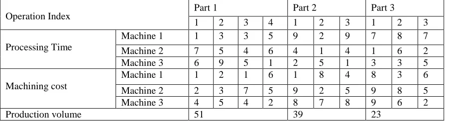
Operation Index Part 1 Part 2 Part 3
1 2 3 4 1 2 3 1 2 3
Processing Time
Machine 1 1 3 3 5 9 2 9 7 8 7 Machine 2 7 5 4 6 4 1 4 1 6 2 Machine 3 6 9 5 1 2 5 1 3 3 5
Machining cost
Machine 1 1 2 1 6 1 8 4 8 3 6 Machine 2 2 3 7 5 9 2 5 9 8 5 Machine 3 4 5 4 2 8 7 8 9 6 2
Production volume 51 39 23
Table.1 Processing time, Machining costs of different operations on 3 machines and production volume of 3
parts
Machine 1 Machine 2 Machine 3
Machine 1 4 11 17
Machine 2 11 3 9
[image:3.612.83.535.134.256.2]Machine 3 7 18 5
Table 2 Travelling time between the Machines
The scheduling of production process by using flexible manufacturing system using three machines with different processing and travelling time at different costs is studied by a numerical calculation. The complexity of the investigation is scheduling
problem in FMS by assuming that all machines are working properly and then some of the machines were stopped working. All these calculations are done by taking different machine indices randomly, large calculations are done.
4. MATHEMATICAL CALCULATIONS
Nomenclature
t1 = Total processing time of three parts in required Production quantity. t2 = Total transportation time in between machines.
F1 = (t1+t2) = Total machining and Transportation time. F2 = Minimization of total too cost.
Sample calculations for
Part Index 1 2 3
Operation Index 1234 123 123
Machine Index 1233 123 132
Step I
a. To find t1 calculations :
t1 = 51 x (1+5+5+1) + 39 x (9+1+1) + 23 x (7+3+2) = 51 x 12 + 39 x 11 + 23 x 12
= 612 + 429 + 276 = 1317. b. To find t2:
t1 = 51/10 x (11+9+5) + 39/10 x (11+9) + 23/10 x (17+18) = 5.1 x 25 + 3.9 x 20 + 2.3 x 35
= 127.5 + 78 + 80.5 = 286.
F1 = f1 + f2
[image:3.612.128.485.289.349.2]251
Step II to find F2:
F2 = (1+3+4+2) + (1+2+8) + (8+6+5) = 10 + 11 + 19 = 40
5. RESULTS AND DISCUSSIONS
5.1 Results
The proposed approach can be used to study the optimization in case of failure of few machines. Results for random sequence of operations,
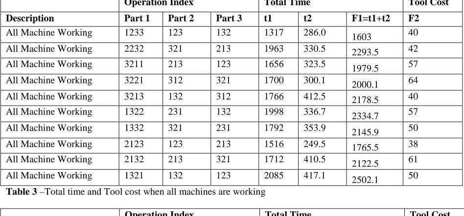
Operation Index Total Time Tool Cost
Description Part 1 Part 2 Part 3 t1 t2 F1=t1+t2 F2
All Machine Working 1233 123 132 1317 286.0 1603 40 All Machine Working 2232 321 213 1963 330.5 2293.5 42 All Machine Working 3211 213 123 1656 323.5 1979.5 57 All Machine Working 3221 312 321 1700 300.1 2000.1 64 All Machine Working 3213 132 312 1766 412.5 2178.5 40 All Machine Working 1322 231 132 1998 336.7 2334.7 57 All Machine Working 1332 321 231 1792 353.9 2145.9 50 All Machine Working 2123 123 213 1516 249.5 1765.5 38 All Machine Working 2132 213 321 1712 410.5 2122.5 61 All Machine Working 1321 132 123 2085 417.1 2502.1 50
Table 3 –Total time and Tool cost when all machines are working
Operation Index Total Time Tool Cost
Description Part 1 Part 2 Part 3 t1 t2 F1=t1+t2 F2
[image:4.612.66.540.229.450.2]Machine 1 Fails 2323 223 323 1627 292.5 1919.5 54 Machine 1 Fails 2332 322 332 1834 298.0 2132 52 Machine 1 Fails 2232 233 322 1816 255.9 2071.9 60 Machine 1 Fails 2233 232 233 1632 224.2 1856.2 56 Machine 1 Fails 2322 332 232 1893 304.8 2197.8 59 Machine 1 Fails 3323 323 223 1452 296.1 1748.1 55 Machine 1 Fails 3223 223 323 1372 261.9 1633.9 54 Machine 1 Fails 3332 233 332 1900 250.3 2150.3 62 Machine 1 Fails 3232 332 322 1804 367.5 2171.5 58 Machine 1 Fails 3233 323 233 1230 300.7 1530.7 48
Table 4 –Total time and Tool cost when machine 1 fails
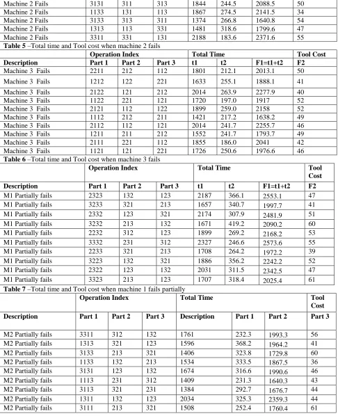
Operation Index Total Time Tool Cost
Description Part 1 Part 2 Part 3 t1 t2 F1=t1+t2 F2
Machine 2 Fails 1131 113 313 1550 279.9 1829.9 44 Machine 2 Fails 3111 331 133 1836 173.9
252 Machine 2 Fails 3131 311 313 1844 244.5 2088.5 50
Machine 2 Fails 1133 131 113 1867 274.5 2141.5 34 Machine 2 Fails 3133 313 311 1374 266.8 1640.8 54 Machine 2 Fails 1313 113 331 1481 318.6 1799.6 47 Machine 2 Fails 3311 331 131 2188 183.6 2371.6 55
Table 5 –Total time and Tool cost when machine 2 fails
Operation Index Total Time Tool Cost
Description Part 1 Part 2 Part 3 t1 t2 F1=t1+t2 F2
Machine 3 Fails 2211 212 112 1801 212.1 2013.1 50 Machine 3 Fails 1212 122 221 1633 255.1 1888.1 41 Machine 3 Fails 2122 121 212 2014 263.9 2277.9 40 Machine 3 Fails 1122 221 121 1720 197.0 1917 52 Machine 3 Fails 2121 112 122 1899 259.0 2158 52 Machine 3 Fails 1112 212 211 1421 217.2 1638.2 49 Machine 3 Fails 2112 112 121 2014 241.7 2255.7 46 Machine 3 Fails 1211 211 212 1552 241.7 1793.7 49 Machine 3 Fails 2111 221 112 1855 186.0 2041 42 Machine 3 Fails 1121 121 221 1726 250.6 1976.6 46
Table 6 –Total time and Tool cost when machine 3 fails
Operation Index Total Time Tool
Cost
Description Part 1 Part 2 Part 3 t1 t2 F1=t1+t2 F2
M1 Partially fails 2323 132 123 2187 366.1 2553.1 47 M1 Partially fails 3233 321 213 1657 340.7 1997.7 41 M1 Partially fails 2332 123 321 2174 307.9 2481.9 51 M1 Partially fails 3232 213 132 1671 419.2 2090.2 60 M1 Partially fails 2232 312 123 1899 269.2 2168.2 53 M1 Partially fails 3332 231 312 2327 246.6 2573.6 55 M1 Partially fails 2233 321 213 1708 264.2 1972.2 39 M1 Partially fails 3223 132 321 1886 356.2 2242.2 52 M1 Partially fails 2322 123 132 2031 311.5 2342.5 47 M1 Partially fails 3323 213 123 1707 318.4 2025.4 61
Table 7 –Total time and Tool cost when machine 1 fails partially
Operation Index Total Time Tool
Cost
Description Part 1 Part 2 Part 3 Description Part 1 Part 2 Part 3
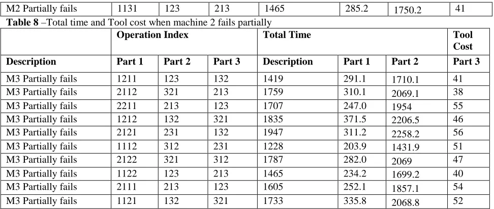
[image:5.612.67.553.122.720.2]253 M2 Partially fails 1131 123 213 1465 285.2 1750.2 41
Table 8 –Total time and Tool cost when machine 2 fails partially
Operation Index Total Time Tool
Cost
Description Part 1 Part 2 Part 3 Description Part 1 Part 2 Part 3
M3 Partially fails 1211 123 132 1419 291.1 1710.1 41 M3 Partially fails 2112 321 213 1759 310.1 2069.1 38 M3 Partially fails 2211 213 123 1707 247.0 1954 55 M3 Partially fails 1212 132 321 1835 371.5 2206.5 46 M3 Partially fails 2121 231 132 1947 311.2 2258.2 56 M3 Partially fails 1112 312 231 1228 203.9 1431.9 51 M3 Partially fails 2122 321 312 1787 282.0 2069 47 M3 Partially fails 1122 123 213 1465 234.2 1699.2 40 M3 Partially fails 2111 213 123 1605 252.1 1857.1 54 M3 Partially fails 1121 132 321 1733 335.8 2068.8 52
Table 8 –Total time and Tool cost when machine 2 fails partially
5.2 Discussion
Formulation of problem:
In this paper, an attempt is made by considering some additional constrains like all machines are working, first machine is not working, second machine is not working, and third machine is not working.
We also done the calculations related to the conditions when any one of the machine get stopped working, like machine one partially failed, machine two partially failed and machine three partially failed. These working conditions are considered by taking the various operational indices on different machines by randomly selection. By taking all these constraints, corresponding objective function values i.e.F1 and F2 are calculated.
Another important constraint we have taken is a machine does not work while manufacturing a particular product, but it works while manufacturing of other two products. We have also considered other conditions like, Machine 1 completely fails, Machine 2 completely fails and Machine 3 fails completely.
• When all machines are working: The
results show that operation index 1233, 123, 132 gives the least manufacturing time for manufacturing of three types of products. And this operation index gives the minimum total tool cost.
• When machine one fails: The results show
that operation index 3233, 323, 233 gives the least manufacturing time for manufacturing of three types of products,
and this operation index gives the minimum total tool cost.
• When machine two fails: The results show
that operation index 3113, 313, 131 gives the least manufacturing time for manufacturing of three types of products, and the operation index 1131, 113, 313 gives the total tool cost minimum.
• When machine three fails: The results
show that operation index 1112, 212, 211 gives the least manufacturing time for manufacturing of three types of products, and the operation index 2122, 121, 212 gives the total tool cost minimum.
• When machine one partially fails: The
results show that operation index 2233, 321, 213 gives the least manufacturing time for manufacturing of three types of products, and this operation index gives the minimum total tool cost.
• When machine two partially fails: The
results show that operation index 1113, 231, 312 gives the least manufacturing time for manufacturing of three types of products, and operation index 1133, 132, 213 gives the total tool cost minimum.
• When machine three partially fails: The
254
6. CONCLUSIONS
The paper identified the different operations index on machines in production planning of Flexible manufacturing system by considering the objective functions as minimizing the manufacturing time, flow time and total tool cost. The objective function values are calculated for randomly selected operation index sequence when all the three machines are working, when machine one fails, machine two fails, machine three fails and machine one partially fails, machine two partially fails, machine partially fails. The results show that when all the machines are working, the objective function values are better for operations indexes 1233, 123, 132 for manufacturing of three parts i.e. Part A, B&C. From the tabulated results it is observed that when machine one fails the values of F1, F2 i.e. total flow time and tool cost is better than the machine two and machine three fails that means it is advisable to maintain the machine two, three properly to avoid failures. The tool cost that is F2 is better when machine two fails and machine three partially fails. From the results it is observed that any one single operation index is not fulfilling both the objectives. But we can suggest the best operation index for the minimization of total flow time and tool cost. Depending upon their objective function we can select the operation index while doing the production planning. In future we are planning to develop an algorithm for identifying better operation index that depending on the objective function that can be achieved when all machines are working or if any one of the machine get failed.
REFERENCES :
[1] Jian-Hung Chen, Shinn-Ying Ho from the paper “A novel approach to production planning of flexible manufacturing systems using an efficient multi-objective genetic algorithm” International Journal of Machine Tools & Manufacture. 45(2005) 945-957. [2] K.Mallikarjuna. V.Veeranna.
K.Hemachandra Reddy “Multi-objective optimization for design of single row layout in flexible manufacturing system with scheduling constraint: an approach of nontraditional optimization techniques” International Journal of Applied Research in Mechanical Engineering.(IJARME) ISSN: 2231-5950, Vol-3, Iss-2, 2013.
[3] Imran Ali Chaudhry and Abdul Munem Khan “Minimizing makespan for a no-wait
flowshop using genetic algorithm” sa-dhana-Vol.37, Part 6, December 2012, pp.695-707.-c Indian Academy of Sciences.
[4] Rajkiran Bramhane, Arun Aroral and H Chandra “Simulation of flexible manufacturing system using adaptive neuro fuzzyhybrid structure for efficient job sequencing and routing” Int.J.Mech.Eng.& Rob. Res.2014
[5] Omar Selt “Numerical solution for solving scheduling problem” Global Journal of Pure and Applied Mathematics. ISSN 0973-1768 Volume 12, Number 5 (2016), pp.4325-4333 [6] P. Kumar, N.K. Tewari, N. Singh, Joint consideration of grouping and loading problems in a flexible manufacturing system, International Journal of Production Research 28 (7) (1990) 1345–1356.
[7] R. Swarnkar, M.K. Tiwari, Modeling machine loading problem of FMSs and its solution methodology using a hybrid tabu search and simulated annealing-based heuristic approach, Robotics and Computer-Integrated Manufacturing 20 (3) (2004) 199–209