Unsupervised Learning of Morphology Using a Novel Directed Search
Algorithm: Taking the First Step
Matthew G. Snover and Gaja E. Jarosz and Michael R. Brent
Department of Computer Science Washington University St Louis, MO, USA, 63130-4809
ms9, gaja, brent @cs.wustl.edu
Abstract
This paper describes a system for the un-supervised learning of morphological suf-fixes and stems from word lists. The sys-tem is composed of a generative probabil-ity model and a novel search algorithm. By examining morphologically rich sub-sets of an input lexicon, the search identi-fies highly productive paradigms. Quanti-tative results are shown by measuring the accuracy of the morphological relations identified. Experiments in English and Polish, as well as comparisons with other recent unsupervised morphology learning algorithms demonstrate the effectiveness of this technique.
1 Introduction
There are numerous languages for which no anno-tated corpora exist but for which there exists an abundance of unannotated orthographic text. It is extremely time-consuming and expensive to cre-ate a corpus annotcre-ated for morphological structure by hand. Furthermore, a preliminary, conservative analysis of a language’s morphology would be use-ful in discovering linguistic structure beyond the word level. For instance, morphology may provide information about the syntactic categories to which words belong, knowledge which could be used by parsing algorithms. From a cognitive perspective, it is crucial to determine whether the amount of infor-mation found in pure speech is sufficient for discov-ering the level of morphological structure that chil-dren are able to find without any direct supervision.
Thus, we believe the task of automatically discover-ing a conservative estimate of the orthographically-based morphological structure in a language inde-pendent manner is a useful one.
Additionally, an initial description of a lan-guage’s morphology could provide a starting point for supervised morphological mod-els, such as the memory-based algorithm of Van den Bosch and Daelemans (1999), which can-not be used on languages for which ancan-notated data is unavailable.
During the last decade several minimally super-vised and unsupersuper-vised algorithms that address the problem have been developed. Gaussier (1999) de-scribes an explicitly probabilistic system that is based primarily on spellings. It is an unsupervised algorithm, but requires the tweaking of parameters to tune it to the target language. Brent (1993) and Brent et al. (1995), described Minimum Description Length, (MDL), systems. One approach used only the spellings of the words; another attempted to find the set of suffixes in the language used the syntactic categories from a tagged corpus as well. While both are unsupervised, the latter is not knowledge free and requires data that is tagged for part of speech, making it less suitable for analyzing under examined languages.
A similar MDL approach is described by Goldsmith (2001). It is ideal in being both knowl-edge free and unsupervised. The difficulty lies in Goldsmith’s liberal definition of morphology which he uses to evaluate with; a more conservative ap-proach would seem to be a better hypothesis to boot-strap from.
which uses a generative probability model and a hill climbing search. No quantitative studies had been conducted on it, and it appears that the hill-climbing search used limits that system’s usefulness. We have developed a system based on a novel search and an extension of the previous probability model of Snover and Brent.
The use of probabilistic models is equivalent to minimum description length models. Searching for the most probable hypothesis is just as compelling as searching for the smallest hypothesis and a model formulated in one framework can, through some mathematical manipulation, be reformulated into the other framework. By taking the negative log of a probability distribution, one can find the number of bits required to encode a value according to that dis-tribution. Our system does not use the minimum de-scription length principle but could easily be refor-mulated to do so.
Our goal in designing this system, is to be able to detect the final stem and suffix break of each word given a list of the most common words in a language. We do not distinguish between derivational and in-flectional suffixation or between the notion of a stem and a base. Our probability model differs slightly from that of Snover and Brent (2001), but the main difference is in the search technique. We find and analyze subsets of the lexicon to find good solutions for a small set of words. We then combine these sub-hypotheses to form a morphological analysis of the entire input lexicon. We do not attempt to learn pre-fixes, inpre-fixes, or other more complex morphological systems, such as template-based morphology: we are attempting to discover the component of many morphological systems that is strictly concatenative. Finally, our model does not currently have a mecha-nism to deal with multiple interpretations of a word, or to deal with morphological ambiguity.
2 Probability Model
This section introduces a prior probability distribu-tion over the space of all hypotheses, where a hy-pothesis is a set of words, each with morphological split separating the stem and suffix. The distribution is based on a seven-model model for the generation of hypothesis, which is heavily based upon the prob-ability model presented in Snover and Brent (2001),
with steps 1-3 of the generative procedure being the same. The two models diverge at step 4 with the pairing of stems and suffixes. Whereas the previ-ous model paired individual stems with suffixes, our new model uses the abstract structure of paradigms. A paradigm is a set of suffixes and the stems that attach to those suffixes and no others. Each stem is in exactly one paradigm, and each paradigm has at least one stem. This is an important improvement to the model as it takes into account the patterns in which stems and suffixes attach.
The seven steps are presented below, along with their probability distributions and a running exam-ple of how a hypothesis could be generated by this process. By taking the product over the distributions from all of the steps of the generative process, one can calculate the prior probability for any given hy-pothesis. What is described in this section is a math-ematical model and not an algorithm intended to be run.
1. Choose the number of stems, , according to the distribution:
(1)
The
term normalizes the inverse-squared distribution on the positive integers. The num-ber of suffixes, is chosen according to the same probability distribution. The symbols M for steMs and X for suffiXes are used through-out this paper.
Example: = 5. = 3.
2. For each stem, choose its length in letters , according to the inverse squared distribution. Assuming that the lengths are chosen indepen-dently and multiplying together their probabil-ities we have:
"!$#
(2)
The distribution for the lengths of the suffixes,
% , is similar to (2), differing only in that suf-fixes of length 0 are allowed, by offsetting the length by one.
3. Let be the alphabet, and let #
be a
probability distribution on . For each from 1 to , generate stem by choosing let-ters at random, according to the probabilities
#
. Call the resulting stem set STEM. The suffix set SUFF is generated in the same manner. The probability of any character,, be-ing chosen is obtained from a maximum likeli-hood estimate: where
is the count of among all the hypoth-esized stems and suffixes and
. The joint probability of the hypothesized stem and suffix sets is defined by the distribution:
STEM SUFF
% "!$# (3)
The factorial terms reflect the fact that the stems and suffixes could be generated in any order.
Example: STEM = walk, look, door, far, cat . SUFF = ed, % , s .
4. We now choose the number of paradigms, & , which can range from 1 to since each stem is in exactly one paradigm, and each paradigm has at least one stem. We pick & according to the following uniform distribution:
& ' # (4)
Example: & = 3.
5. We choose the number of suffixes in the paradigms,( , according to a uniform distribu-tion. The distribution for picking (
, suffixes for paradigm is:
( )&
The joint probability over all paradigms, ( is therefore: ( *& ,+ "!$# ' # + (5)
Example: ( = 2, 1, 2 .
6. For each paradigm, choose the set of( suf-fixes, PARA% that the paradigm will represent. The number of subsets of a given size is finite so we can again use the uniform distribution. This implies that the probability of each indi-vidual subset of size (
, is the inverse of the total number of such subsets. Assuming that the choices for each paradigm are independent:
PARA% *&-( + !$# ( ' # ( ' + (6)
Example: PARA%# =
.% , s, ed . PARA
%
= .%/ . PARA% 0 =.% , s .
7. For each stem choose the paradigm that the stem will belong in, according to a distribution that favors paradigms with more stems. The probability of choosing a paradigm, for a stem is calculated using a maximum likelihood esti-mate:
PARA
where PARA is the set of stems in paradigm
. Assuming that all these choices are made in-dependently yields the following:
PARA *& + "!$# PARA PARA12 (7)
Example: PARA# =
walk, look . PARA
=
far . PARA0 = door, cat .
Combining the results of stages 6 and 7, one can see that the running example would yield the hy-pothesis consisting of the set of words with suffix breaks, walk+% , walk+s, walk+ed, look+% , look+s, look+ed, far+% , door+% , door+s, cat+% , cat+s . Re-moving the breaks in the words results in the set of input words. To find the probability for this hypoth-esis just take of the product of the probabilities from equations (1) to (7).
distribution over the positive integers, that slightly favors smaller numbers. Experiments substitut-ing the universal prior for integers, developed by Rissanen (1989), for the inverse squared distribu-tion, have shown that the model is not sensitive to the exact distribution used for these steps. Only slight differences in the some of the final hypotheses were found, and it was unclear which of the methods pro-duced superior results. The reason for the lack of effect is that the two distributions are not too dis-similar and steps 1 and 2 are not main contributors to the probability mass of our model. Thus, for the sake of computational simplicity we use the inverse squared distribution for these steps.
Using this generative model, we can assign a probability to any hypothesis. Typically one wishes to know the probability of the hypothesis given the data, however in our case such a distribution is not required. Equation (8) shows how the probability of the hypothesis given the data could be derived from Bayes law.
Hyp Data
Hyp
Data Hyp
Data
(8)
Our search only considers hypotheses consistent with the data. The probability of the data given the hypothesis,
DataHyp
, is always
, since if you remove the breaks from any hypothesis, the in-put data is produced. This would not be the case if our search considered inconsistent hypotheses. The prior probability of the data is unknown, but is con-stant over all hypotheses, thus the probability of the hypothesis given the data reduces to
Hyp
. The prior probability of the hypothesis is given by the above generative process and, among all consis-tent hypotheses, the one with the greatest prior prob-ability also has the greatest posterior probprob-ability.
3 Search
This section details a novel search algorithm which is used to find the most likely segmentation of the all the words in the input lexicon, . The input lexicon is a list of words extracted from a corpus. The output of the search is a segmentation of each of the input words into a stem and suffix. The algorithm does not directly attempt to find the most probable hypothesis
consistent with the input, but finds a highly probable consistent hypothesis.
The directed search is accomplished in two steps. First sub-hypotheses, each of which is a hypothe-sis about a subset of the lexicon, are examined and ranked. The best sub-hypotheses are then incmentally combined until a single sub-hypothesis re-mains. The remainder of the input lexicon is added to this sub-hypothesis at which point it becomes the final hypothesis.
3.1 Ranking Sub-Hypotheses
We define the set of possible suffixes to be the set of terminal substrings, including the empty string
% , of the words in . Each subset of the possible suffixes has a corresponding sub-hypothesis. The sub-hypothesis, , corresponding to a set of suffixes SUFF , has the set of stems STEMS . For each stem and suffix , in , the word must be a word in the input lexicon. STEM is the max-imal sized set of stems that meets this requirement. The sub-hypothesis, , is thus the hypothesis over the set of words formed by all pairings of the stems in STEM and the suffixes in SUFF with the cor-responding morphological breaks. One can think of each sub-hypothesis as initially corresponding to a maximally filled paradigm. We only consider sub-hypotheses which have at least two stems and two suffixes.
For each sub-hypothesis, , there is a correspond-ing counter hypothesis, , which has the same set of words as , but in which all the words are hypothe-sized to consist of the word as the stem and% as the suffix.
We can now assign a score to each sub-hypothesis as follows: score
. This reflects how much more probable is for those words, than the counter or null hypothesis.
One can view all sub-hypotheses as nodes in a di-rected graph. Each node, , is connected to another node, if and only if represents a superset of the suffixes that represents, which is exactly one suf-fix greater in size than the set that represents. By beginning at the node representing no suffixes, one can apply standard graph search techniques, such as a beam search or a best first search to find the best scoring nodes without visiting all nodes. While one cannot guarantee that such approaches perform exactly the same as examining all sub-hypotheses, initial experiments using a beam search with a beam size equal to , with a of 100, show that the best sub-hypotheses are found with a significant de-crease in the number of nodes visited. The experi-ments presented in this paper do not use these prun-ing methods.
3.2 Combining Sub-Hypotheses
The highest scoring sub-hypotheses are incre-mentally combined in order to create a hypothesis over the complete set of input words. The selection of should not vary from language to language and is simply a way of limiting the computational com-plexity of the algorithm. Changing the value of does not dramatically alter the results of the algo-rithm, though higher values of give slightly better results. We let be 100 in the experiments reported here.
Let
be the set of the highest scoring sub-hypotheses. We remove from
the sub-hypothesis,
, which has the highest score. The words in are now added to each of the remaining sub-hypotheses in
, and their counter hypotheses. Every sub-hypothesis,
, and its counter,
, in
are modified such that they now contain all the words from
with the morphological breaks those words had in
. If a word was already in
and
and it is also in then it now has the morphological break from
, overrid-ing whatever break was previously attributed to the word.
All of the sub-hypotheses now need to be rescored, as the words in them will likely have changed. If, after rescoring, none of the sub-hypotheses have scores greater than one, then we use
as our final hypothesis. Otherwise we repeat the process of selecting
and adding it in. We con-tinue doing this until all sub-hypotheses have scores
of one or less or there are no sub-hypotheses left. The final sub-hypothesis,
, is now converted into a full hypothesis over all the words. All words in , that are not in
are added to
with% as their suffix. This results in a hypothesis over all the words in .
4 Experiment and Evaluation
4.1 Experiment
We tested three unsupervised morphology learning systems on various sized word lists from English and Polish corpora. For English we used set A of the Hansard corpus, which is a parallel English and French corpus of proceedings of the Canadian Par-liament. We were unable to find a standard corpus for Polish and developed one from online sources. The sources for the Polish corpus were older texts and thus our results correspond to a slightly anti-quated form of the language. We compared our di-rected search system, which consists of the prob-ability model described in Section 2 and the di-rected search described in Section 3 with Gold-smith’s MDL algorithm, otherwise known as Lin-guistica1 and our previous system (2001), which
shall henceforth be referred to as the Hill Climbing Search system. The results were then evaluated by measuring the accuracy of the stem relations identi-fied.
We extracted input lexicons from each corpus, ex-cluding words containing non-alphabetic characters. The 100 most common words in each corpus were also excluded, since these words tend to be function words and are not very informative for morphology. Including the 100 most common words does not sig-nificantly alter the results presented. The systems were run on the 500, 1,000, 2,000, 4,000, and 8,000 most common remaining words. The experiments in English were also conducted on the 16,000 most common words from the Hansard corpus.
4.2 Evaluation Metrics
Ideally, we would like to be able to specify the cor-rect morphological break for each of the words in the input, however morphology is laced with ambiguity,
1
and we believe this to be an inappropriate method for this task. For example it is unclear where the break in the word, “location” should be placed. It seems that the stem “locate” is combined with the suffix “tion”, but in terms of simple concatenation it is unclear if the break should be placed before or after the “t”. When “locate” is combined with the suffix “s”, simple concatenation seems to work fine, though a different stem is found from “location” and the suffix “es” could be argued for. One solution is to develop an evaluation technique which incorporates the adjustment or spelling change rules, such as the one that deletes the “e” in “locate” when combining with “tion”.
None of the systems being evaluated attempt to learn adjustment rules, and thus it would be diffi-cult to analyze them using such a measure. In an attempt to solve this problem we have developed a new measure of performance, which does not spec-ify the exact morphological split of a word. We mea-sure the accuracy of the stems predicted by examin-ing whether two words which are morphologically related are predicted as having the same stem. The accuracy of the stems predicted is analyzed by ex-amining whether pairs of words are morphologically related by having the same immediate stem. The ac-tual break point for the stems is not evaluated, only whether the words are predicted as having the same stem. We are working on a similar measure for suf-fix identification, which measures whether pairs that have the same suffix are found as having the same suffix, regardless of the actual form of the suffix pre-dicted.
4.2.1 Stem Relation
Two words are related if they share the same im-mediate stem. For example the words “building”, “build”, and “builds” are related since they all have “build” as a stem, just as “building” and “build-ings” are related as they both have “building” as a stem. The two words, “buildings” and “build” are not directly related since the former has “building” as a stem, while “build” is its own stem. Irregular forms of words are also considered to be related even though such relations would be very difficult to de-tect with a simple concatenation model.
We say that a morphological analyzer predicts two words as being related if it attributes the same
stem to both words, regardless of what that stem ac-tually is. If an analyzer made a mistake and said both “build’ and “building” had the stem “bu”, we would still give credit to it for finding that the two are related, though this analysis would be penalized by the suffix identification measure. The stem rela-tion precision measures how many of the relarela-tions predicted by the system were correct, while the re-call measures how many of the relations present in the data were found. Stem relation fscore is an unbi-ased combination of precision and recall that favors equal scores.
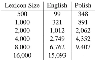
Lexicon Size English Polish
500 99 348
1,000 321 891
2,000 1,012 2,062 4,000 2,749 4,352 8,000 6,762 9,407 16,000 15,093
-Table 1: Correct Number of Stem Relations
The correct number of stem relations for each lex-icon size in English and Polish are shown in Table 1. Because Polish has a richer morphology than En-glish, the number of relations in Polish is signifi-cantly higher than the number of relations in English at every lexicon size.
4.3 Results
The results from the experiments are shown in Fig-ures 1- 3. All graphs are shown use a log scale for the corpus size. Due to software difficulties we were unable to get Linguistica to run on 500, 1000, and 2000 words in English. The software ran without difficulties on the larger English datasets and on the Polish data.
[image:6.612.348.503.245.343.2]0 100 200 300 400 500 600 700 800
500 1000 2k 4k 8k 16k
English Number of Suffixes
Lexicon Size
0 20 40 60 80 100 120 140 160
500 1000 2k 4k 8k
Polish Number of Suffixes
Lexicon Size Directed Search
[image:7.612.151.462.72.245.2]Linguistica Hill Climbing Search
Figure 1: Number of Suffixes Predicted
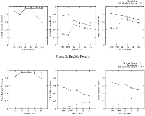
Figure 2 shows the precision, recall and fscore using the stem relation metric. Figure 3 shows the performance of the algorithms on the Polish input lexicon. The Hill Climbing Search system was un-able to learn any morphology on the Polish data sets, and thus has zero precision and recall. The Directed Search maintains a very high precision across lexi-con sizes in both languages, whereas the precision of Linguistica decreases considerably at larger lexicon sizes. However Linguistica shows an increasing re-call as the lexicon size increases, with our Directed Search having a decreasing recall as lexicon size in-creases, though the recall of Linguistica in Polish is consistently lower than the Directed Search system’s recall. The fscores for the Directed Search and Lin-guistica in English are very close, and the Directed Search appears to clearly outperform Linguistica in Polish.
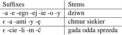
Suffixes Stems
-a -e -ego -ej -ie -o -y dziwn
% -a -ami -y -e¸ chmur siekier
[image:7.612.88.285.543.600.2]% -cie -li -m -´c gada odda sprzeda
Table 2: Sample Paradigms in Polish
Table 2 shows several of the larger paradigms found by our directed search algorithm when run on 8000 words of Polish. The first paradigm shown is for the single adjective stem meaning “strange” with numerous inflections for gender, number and case, as well as one derivational suffix, “-ie” which
changes it into an adverb, “strangely”. The sec-ond paradigm is for the nouns, “cloud” and “ax”, with various case inflections and the third paradigm paradigm contains the verbs, “talk”, “return”, and “sell”. All suffixes in the third paradigm are inflec-tional indicating tense and agreement.
As an additional note, Linguistica was dramati-cally faster than either our Directed Search or the Hill Climbing Search system. Both systems are de-velopment oriented software and not as optimized for efficient runtime as Linguistica appears to be.
Of the three systems, the Hill Climbing Search system has poorest performance. The poor perfor-mance of the Hill Climbing Search system in Polish is due to a quirk in its search algorithm, which pre-vents it from hypothesizing stems that are not them-selves words. This is not a bug in the software, but a property of the algorithm used. In English this is not a significant difficulty as most stems are also words, but this is almost never the case in Polish, where al-most all stems require some suffix.
sys-0 0.2 0.4 0.6 0.8 1
500 1000 2k 4k 8k 16k
English Relation Recall
Lexicon Size 0
0.2 0.4 0.6 0.8 1
500 1000 2k 4k 8k 16k
English Relation Precision
Lexicon Size
0 0.2 0.4 0.6 0.8 1
500 1000 2k 4k 8k 16k
English Relation Fscore
Lexicon Size Directed Search
[image:8.612.69.541.78.458.2]Linguistica Hill Climbing Search
Figure 2: English Results
0 0.2 0.4 0.6 0.8 1
500 1000 2k 4k 8k
Polish Relation Precision
Lexicon Size
Polish Relation Recall
0 0.2 0.4 0.6 0.8 1
500 1000 2k 4k 8k Lexicon Size
Polish Relation Fscore
0 0.2 0.4 0.6 0.8 1
500 1000 2k 4k 8k Lexicon Size
Directed Search Linguistica Hill Climbing Search
Figure 3: Polish Results
tem for morphological analysis, where the number of false positives is minimized.
Most of Linguistica’s errors in English resulted from the algorithm mistaking word compounding, such as “breakwater”, for suffixation, namely treat-ing “water” as a productive suffix. While we do think that the word compounding detected by Lin-guistica is useful, such compounding of words is not generally considered suffixation, and thus should be penalized against.
The Polish language presents special difficulties for both Linguistica and our Directed Search sys-tem, due to the highly complex nature of its mor-phology. There are far fewer spelling change rules and a much higher frequency of suffixes in Polish than in English. In addition phonology plays a much
stronger role in Polish morphology, causing alter-ations in stems, which are difficult to detect using a concatenative framework.
5 Discussion
Experiments substituting the inverse squared distri-bution with the universal prior have shown no sig-nificant empirical difference in performance. We are currently working on a more detailed comparison of the two systems.
The results obtained from Directed Search al-gorithm can be significantly improved by in-corporating the hill climbing search detailed in Snover and Brent (2001). The hill climbing search attempts to move stems from one paradigm to sim-ilar paradigms to increase the probability of the hy-pothesis. Experiments where the hypothesis out-putted by the Directed Search system is used as the starting hypothesis for the hill climbing search, using the probability model detailed in this paper, show an increase in performance, most notably in recall and fscore, over using the Directed Search in isolation.
Many of the stem relations predicted by the Di-rected Search algorithm, result from postulating stem and suffix breaks in words that are actually morphologically simple. This occurs when the end-ings of these words resemble other, correct, suffixes. In an attempt to deal with this problem we have in-vestigated incorporating semantic information into the probability model since morphologically related words also tend to be semantically related. A suc-cessful implementation of such information should eliminate errors such as “capable” breaking down as “cap”+”able” since “capable” is not semantically re-lated to “cape” or “cap”.
Using latent semantic analysis, Schone and Jurafsky (2000) have previously demonstrated the success of using semantic in-formation in morphological analysis. Preliminary results on our datasets using a similar technique, co-occurrence data, which represents each word as a vector of frequencies of co-occurrence with other words, indicates that much semantic, as well as morphological, information can be extracted. When the cosine measure of distance is used in comparing pairs of words in the corpus, the highest scoring pairs are for the most part morphologically or semantically related. We are currently working on correctly incorporating this information into the probability model.
The Directed Search algorithm does not currently handle multiple suffixation or any prefixation;
how-ever, some ideas for future work involve extend-ing the model to capture these processes. While such an extension would be a significant one, it would not change the fundamental nature of the al-gorithm. Furthermore, the output of the present system is potentially useful in discovering spelling change rules, which could then be bootstrapped to aid in discovering further morphological structure. Yarowsky and Wicentowski (2000) have developed a system that learns such rules given a preliminary morphological hypothesis and part of speech tags.
While the experiments reported here are based on an input lexicon of orthographic representations, there is no reason why the Directed Search algorithm could not be applied to phonetically transcribed data. In fact, especially in the case of the English language, where the orthography is particularly in-consistent with the phonology, our algorithm might be expected to perform better at discovering the in-ternal structure of phonologically transcribed words. Furthermore, phonetically transcribed data would eliminate the problems introduced by the lack of one-to-one correspondence of letters to phonemes. Namely, the algorithm would not mistakenly treat sibilants, such as the /ch/ sound in “chat” as two sep-arate units, although these phonemes are often rep-resented orthographically by a two letter sequence. A model of morphology incorporating phonologi-cal information such as phonologiphonologi-cal features could capture morphological phenomena that bridge the morphology-phonology boundary, such as allophy, or the existence of multiple variants of mor-phemes. Simply running the algorithm on pho-netic data might not improve performance though, as same structures which were more straight forward in the orthographic data might be more complex in the phonetic representation. Finally, for those interested in the question of whether the language learning en-vironment provides children with enough informa-tion to discover morphology with no prior knowl-edge, an analysis of phonological not orthographic data would be necessary.
but more importantly, the precision of Linguistica does not approach the precision of our algorithm, particularly on the larger corpus sizes. On the other hand, we feel the Directed Search algorithm has at-tained the goal of producing an initial estimate of suffixation that could aid other models in discover-ing higher level structure.
References
Michael R. Brent, Sreerama K. Murthy, and Andrew Lundberg. 1995. Discovering morphemic suffixes: A case study in minimum description length induction. In Proceedings of the Fifth International Workshop on
Artificial Intelligence and Statistics, Ft. Laudersdale,
FL.
Michael R. Brent. 1993. Minimal generative models: A middle ground between neurons and triggers. In
Pro-ceedings of the 15th Annual Conference of the Cogni-tive Science Society, pages 28–36, Hillsdale, NJ.
Erl-baum.
´
Eric. Gaussier. 1999. Unsupervised learning of deriva-tional morphology from inflecderiva-tional lexicons. In ACL
’99 Workshop Proceedings: Unsupervised Learning in Natural Language Processing. ACL.
John Goldsmith. 2001. Unsupervised learning of the morphology of a natural language. Computational Linguistics, 27:153–198.
Jorma Rissanen. 1989. Stochastic Complexity in
Statisti-cal Inquiry. World Scientific Publishing, Singapore.
Patrick Schone and Daniel Jurafsky. 2000. Knowledge-free induction of morphology using latent semantic analysis. In Proceedings of the Conference on
Com-putational Natural Language Learning. Conference on
Computational Natural Language Learning.
Matthew G. Snover and Michael R. Brent. 2001. A Bayesian Model for Morpheme and Paradigm Identi-fication. In Proceedings of the 39th Annual Meeting
of the ACL, pages 482–490. Association for
Computa-tional Linguistics.
Antal Van den Bosch and Walter Daelemans. 1999. Memory-based morphological analysis. In Proc. of the
37th Annual Meeting of the ACL. ACL.