S o m e A p p l i c a t i o n s o f T r e e - b a s e d M o d e l l i n g t o S p e e c h a n d L a n g u a g e Michael D. Riley
AT,~T Bell Laboratories
1. I n t r o d u c t i o n
Several applications of statistical tree-based modelling are described here to problems in speech and language. Classification and regression trees are well suited to many of the pattern recognition problems encountered in this area since they (1) statistically select the most significant features involved (2) provide "honest" estimates of their performance, (3) permit both categorical and continuous features to be considered, and (4) allow human interpretation and exploration of their result. First the method is summarized, then its application to automatic stop classification, segment duration prediction for synthesis, phoneme-to-phone classification, and end-of-sentence detection in text are described. For other applications to speech and language, see [Lucassen 1984], [Bahl, et al 1987].
2. C l a s s i f i c a t i o n a n d R e g r e s s i o n T r e e s
An excellent description of the theory and implementation of tree-based statistical models can be found in Classit~cation and Regression Trees [L. Breiman, et al, 1984]. A brief description of these ideas will be provided here.
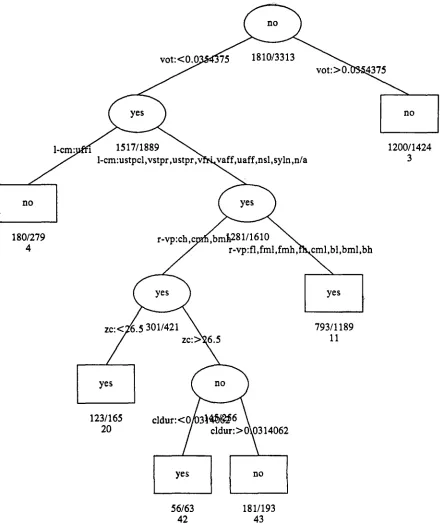
Figure 1 shows an example of a tree for classifying whether a stop (in the context C V) is voiced or voiceless based on factors such as voice onset time, closure duration, and phonetic context. Let us first see how to use such a tree for classification. Then we will see how the tree was generated.
Suppose we have a stop with a V O T of 30 msec that is preceded by a nasal and followed by a high back vowel. Starting at the root node in Figure 1, the first decision is whether the V O T is greater or less than 35.4 msec. Since in our example, it is less, we take the left branch. The next split, labelled "l-cm", refers to the consonantal manner of the the preceding (left) segment. Since in this case it is nasal, we take the right branch. The next split is on the vowel place of following (right) segment. Since it is high back in this case, we take the right branch, reaching a terminal node. The node is labelled "yes", indicating that this example should be classified as voiced.
In the training set, 739 of the 1189 examples that reached this node were correctly classified. This tree is a subtree of a better classifier to be described in the next section; this example was pruned for illustrative purposes.
This is an example of a classification tree, since the decision is to choose one of several classes; in this case, there are two classes: {voiced, voiceless}. In other words, the predicted variable, y, is categorical. Trees can be created for continuous y also. In this case they are called regression trees with the terminal nodes labelled with a real number (or, more generally, a vector).
Voiced or Voiceless Stop?
1810/3313
yes
no
1.cm~
l
~
.
1200/1424
~
1-cm:ustpcl,vstpr,ustpr,vtM~,~f,uaff,nsl,syln,n/a
3,1/
no
c ~
180/279
r-vp:ch,
r.vi
4
):fl,fml,fmh,fhx~ml,bl,bml,bh
yes ,
yes
•
.5 301/421 > ~
793/1189
zc: 6.5
11
123/165
cldur:<j 3 1 ' ~ 6 0 ~
20
cldur:> ,314062
yes
I
no
56/63
181/193
[image:2.612.96.537.88.619.2]42
43
Let us begin answering these questions by introducing some notation. Consider t h a t we have N samples of data, with each sample consisting of M features, xl, x2, x 3 , . . , xm. In the voiced/voiceless stop example, xl might be VOT, x2 the phonetic class of the preceding segment, etc. Just as the y (dependent) variable can be continuous or categorical, so can the x (independent) variables. E.g., V O T is continuous, while phonetic class is categorical (can not be usefully ordered).
The first question - - what stopping rule? - - refers to what split to take at a given node. It has two parts: (a) what candidates should be considered, and (b) which is the best choice among candidates for a given node?
A simple choice is to consider splits based on one x variable at a time. If the independent variable being considered is continuous - o o < x < c~, consider splits of the form:
z _ < k vs. x > k , Vk.
In other words, consider all binary cuts of that variable. If the independent variable is categorical x E {1, 2, ..., n} = X , consider splits of form:
x ~ A vs. x E X - A , V A c X .
In other words, consider all binary partitions of that variable. More sophisticated splitting rules would allow combinations of a such splits at a given node; e.g., linear combinations of continuous variables, or boolean combinations of categorical variables.
A simple choice to decide which of these splits is the best at a given node is to select the one that minimizes the estimated classification or prediction error after that split based on the training set. Since this is done stepwise at each node, this is not guaranteed to be globally optimal even for the training set.
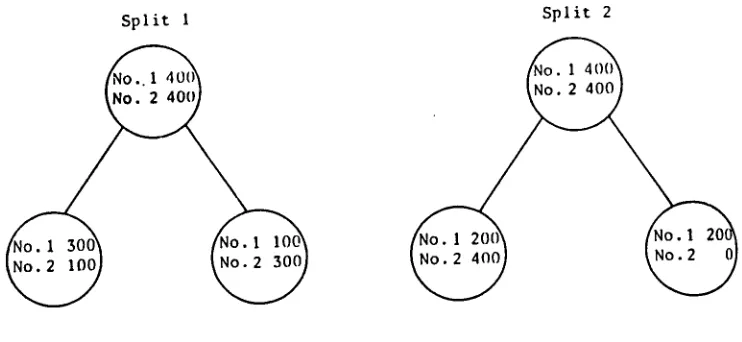
In fact, there are cases where this is a bad choice. Consider Figure 2, where two different splits are illustrated for a classification problem having two classes (No. 1 and No. 2) and 800 samples in the training set (with 400 in each class). If we label each child node according to the greater class present there, we see that the two different splits illustrated both give 200 samples misclassified. Thus, minimizing the error gives no preference to either of these splits.
The example on the right, however, is b e t t e r because it creates at least one very pure node (no misclassifi- cation) which needs no more splitting. At the next split, the other node can be attacked. In other words, the stepwise optimization makes creating purer nodes at each step desirable. A simple way to do this is to minimize the entropy at each node for categorical y. Minimizing the mean square error is a common choice for continuous y.
T h e second question - - what stopping rule? - - refers when to declare a node terminal. Too large trees may match the training d a t a well, but they won't necessarily perform well on new test data, since they have overfit the data. Thus, a procedure is needed to find an "honest-sized" tree.
Early attempts at this tried to find good stopping rules based on absolute purity, differential purity from the parent, and other such "local" evaluations. Unfortunately, good thresholds for these vary from problem to problem.
S p l i t 1 S p l i t 2
F i g u r e 2. Two different splits with the same misclassification rate.
To form the sequence of subtrees in (b), vary c~ from 0 (for full tree) to oo (for just the root node) in: min [ R ( T ) + a l T I ] .
T
where R ( T ) is the classification or prediction error for that subtree and I TI is the number of terminal nodes in the subtree. This is called the cost-complexity pruning sequence.
To estimate an "honest" error rate in (c), test the subtrees on data different from the training data, e.g., grow the tree on 9/10 of the available d a t a and test on 1/10 of the data repeating 10 times and averaging. This is often called cross-validation.
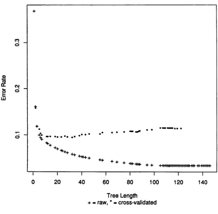
Figure 3 shows misclassification rate vs. tree length for the voiced-voiceless stop classification problem. T h e b o t t o m curve shows misclassification for the training data, which continues to improve with increasing tree length. T h e higher curve shows the cross-validated misclassification rate, which reaches a minimum with a tree size of about 30 and then rises again with increasing tree length. In fact a tree length of around 10 is very near optimal and would be a good choice for this problem.
T h e last question - - what prediction is made at a terminal node? - - is easy to answer. If the predicted variable is categorical, choose the most frequent class among the training samples at that node (plurality vote). If it is continuous, choose the mean of the training samples at that node.
[image:4.612.131.502.45.216.2]Voiced/Voiceless Decision
W d
¢ q d -
O ÷
4.
~ t Q ~ t t Q Q ~ t ~ Q Q
%
QQ Q Q
4 - 4 - ÷ "¢d" -~lt-
Q ~ Q Q Q Q
4. 4- ', :::::::::::::::::::::::: ::: '.: '.::::'.?,
I I I I I I I I
0 20 4 0 60 80 100 120 140
Tree Length
+ = raw, * = cross-vaJidated
F i g u r e 3 .
[image:5.612.99.524.80.498.2]3. S t o p C l a s s i f i c a t i o n
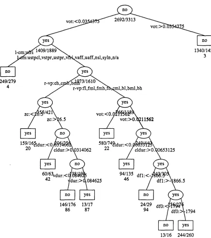
T h e first application has already partially been introduced. Figure 4 shows a more complete tree than Figure 1 for deciding whether a stop is voiced or voiceless. This tree size was selected for the reasons given above. This tree was grown from 3313
stop+vowel
examples taken from male speaker in the T I M I T database. The classification task is to decide whether a given stop was labelled voiced(b, d, g)
or unvoiced(p, t, k)
by the T I M I T transcribers.T h e features (possible zrs) considered were: • Voice Onset Time
• Closure Duration • Vowel Duration
• Zero Crossing Rate between Release and Onset • Phonetic Context:
-- Segment to left: manner/place, consonant/vowel -- Segment to right: m a n n e r / p l a c e
• Vowel Formant Freqs. and Slopes at Onset • F0 and F0 Slope at Onset
T h e first three features were computed directly from the T I M I T labellings. T h e zero-crossing rate was the mean rate between release and onset. T h e formant and F0 values were computed using David Talkin's formant and pitch extraction programs [Talkin 1987].
Coding the phonetic context required special considerations since more than 50 phones (using the T I M I T labelling) can precede a stop in this context. If this were treated as a single feature, more than 25° binary partitions would have to be considered for this variable at each node, clearly making this approach imprac- tical. Chou [1987] proposes one solution, which is to use k-means clustering to find sub-optimal, but good paritions in linear complexity.
The solution adopted here is to classify each phone in terms of 4 features,
consonant manner, consonant
place, "vowel
manner",and "vowel place",
each class taking on about a dozen values. Consonant mannertakes on the usual values such as
voiced fricative, unvoiced stop, nasal, etc.
Consonant manner takes on values such asbilabial,
dental,velar, etc.
"Vowel manner" takes on values such asmonopthong, diphthong,
glide, liquid, etc.
and "vowel place" takes on values such asfront-low, central-mid-high, back-high, etc.
Allcan take on the value " n / a " if they do not apply; e.g., when a vowel is being represented, consonant manner and place are assigned
"n/a".
In this way, every segment is decomposed into four multi-valued features that have acceptable complexity to the classification scheme and that have some phonetic justification.T h e tree in Figure 4 correctly classifies about 91% of the stops as voiced or voiceless. All percent figures quoted in this paper are cross-validated unless otherwise indicated. In other words, they are tested on data distinct from the training data.
Voiced or Voiceless Stop?
VO
2692/3313
l-cm:
n/a
1340/1424
3
249/279
4
r-vp:ch,c
r-vp:fl,fml,fmh, ftbc.ml,bl ,bml,bh
z c ; <
6.5
vot:<0.~2I'P56~:
/
vot:>~
111562
15~/O16~ldur:<O
j
580/74~ldur:< 0
22
)
0653125
60/63vdur:<(
42
94/13546 dfl:<~
866.5
146/176
13/17
86
87
24/29
94
.1794
13/16
244/260
190
191
[image:7.612.95.531.82.572.2]4. S e g m e n t d u r a t i o n m o d e l l i n g f o r s p e e c h s y n t h e s i s
400 utterances from a single speaker and 4000 utterances from 400 speakers (the T I M I T database) of Amer- ican English were used separately to build regression trees t h a t predict segment durations based on the following features:
• Segment Context:
- - Segment to predict
- - Segment to left
- - Segment to right
• Stress (0, 1, 2)
• Word Frequency: (tel. 25M AP words) • Lexical Position:
- - Segment count from start of word - - Segment count from end of word - - Vowel count from start of word - - Vowel count from end of word • Phrasal Position:
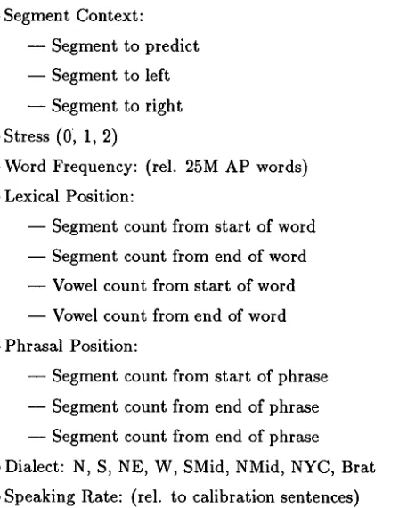
- - Segment count from start of phrase - - Segment count from end of phrase - - Segment count from end of phrase • Dialect: N, S, NE, W, SMid, NMid, NYC, Brat • Speaking Rate: (tel. to calibration sentences)
T h e coding of each segment was decomposed into four features each as described above. T h e word frequency was included as a crude function word detector and was based on six months of AP news text. T h e last two features were used only for the multi-speaker database. T h e stress was obtained from a dictionary (which is easy, but imperfect). T h e dialect information was coded with the T I M I T database. T h e speaking rate is specified as the mean duration of the two calibration sentences, which were spoken by every speaker. Over 70% of the durational variance for the single speaker and over 60% for the multiple speakers were accounted for by these trees. Figure 5 shows durations and duration residuals for all the segments together. Figure 6 shows these broken down into particular phonetic classes. The large tree sizes here, m a n y hundreds of nodes, make t h e m uninteresting to display.
These trees were used to derive durations for a text-to-speech synthesizer and were found to often give more faithful results than the existing heuristically derived duration rules [cf. Klatt 1976]. Since tree building and evaluation is rapid once the data are collected and the candidate features specified, this technique can be readily applied to other feature sets and to other languages.
5. P h o n e m e - t o - p h o n e p r e d i c t i o n
[image:8.612.101.325.107.392.2]Segment Durations
co
8
o
I
0,0
II
I h-I-~
I I f I I
0.05 0.10 0.15 0.20 0.25
seconds
Duration Residuals
~2
o
8
o
I I I
0.0 0.05 0.10 0.15 0.20 0.25
[image:9.612.168.429.73.646.2]Segment Durations by Phonetic Class
d
• • | [
u ~
-
.'
i
,, I;
1
1
o
mono diph vstp uvstp vfdc uvfric vaflr uvaffr liquid glide n a s a l
2 °
~5o
9 i
Duration Residuals by Phonetic Class
EtE tE
; ' ;
, I T
i T
l l
, ' I I
I I
i ' t
t
T
I I I
I I
l
I
|
m o n o diph vstp uvstp vfric uv~ric vatfr uvaffr liquid glide n a s a l
[image:10.612.180.439.69.274.2]T I M I T database. T h e features used for this tree and a larger tree made for all phones were: • Phonemic Context:
- - Phoneme to predict - - Three phonemes to left
-- Three phonemes to right
• Stress (0, 1, 2)
• Word Frequency: (rel. 25M AP words)
• Dialect: N, S, NE, W, SMid, NMid, NYC, Brat • Lexical Position:
-- Phoneme count from start of word -- Phoneme count from end of word
• Phonetic Context: phone predicted to left
The phonemic context was coded in a seven segment window centered on the phoneme to realize, again using the 4 feature decomposition described above (and labelled cm-3, cm-2,..., cm3 ; cp-3, cp-2,..., cp3, etc.). The other features are similar to the duration prediction problem. Ignore the last feature, for the moment. In Figure 7, we can see several cases of how a phonemic T is realized. The first split is roughly whether the segment after the T is a vowel or consonant. If we take the right branch, the next split (to Terminal Node 7) indicates that a nasal, R, or L is almost always unreleased (2090 out 2250 cases) Terminal Node 11 indicates that if the segment preceding the T is a stop or "blank" (beginning of utterance) the T closure is unlabelled, which is the convention adopted by the transcribers. Terminal Node 20 indicates t h a t an intervocalic T preceding an unstressed vowel is often flapped.
This tree predicts about 75% of the phonetic realizations o f T correctly. T h e much larger tree for all phonemes predicts on the average 84% of the T I M I T labellings exactly. A large percentage of the errors are on the precise labelling of reduced vowels as either IX or AX.
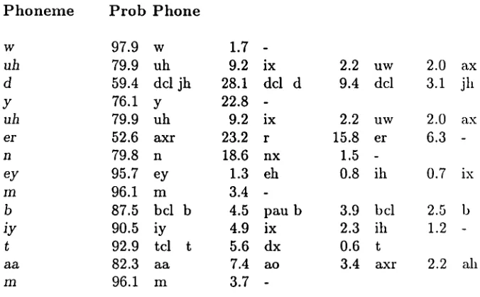
A list of alternative phonetic realizations can also be produced from the tree, since the relative frequencies of different phones appearing at a given terminal node can be computed. Figure 8 shows such a listing for the utterance, Would your name be Tom? . It indicates, for example, that the D in "would" is most likely uttered as a DCL JH in this context (59% of the time), followed by DCL D (28%). On the average four alternatives per phoneme are sufficient to cover 99% of the possible phonetic reMizations. This can be used, for example, to greatly constrain the number of alternatives that must be considered in automatic segmentation when the orthography is known.
These a priori probabilities, however, do not take into account the phonetic context, only the phonemic. For example, if DCL J t t is uttered for the D in the example in Figure 7, then Y is most likely deleted and not uttered. However, the overall probability that a Y is uttered in that phonemic context (averaging both D going to DCL Jii, D, etc.) is greatest. The point is that to incorporate the fact t h a t "D goes to DCL JH implies Y usually deletes" is that transition probabilities should be taken into account.
Phonetic Realization of T
vm I :mono
4257/7183
vml:
era- 1 :vfri,
798/1533
4
2139/4012
v m - 1 : m o n o
~,rho,n/a
cm-1
cpl:blab,labd,
.,ufri,vaff,~aff
cm-l:nas,~,lat,n/a
\
2090/2250
l,vel
7
~a,n/a
rstr:
sec
481/733
11
176/416
12
tcl+t ]
214/505
13
dx I
389/899
20
rseg:
[ tcl+t
259/369
257/478
42
43
[image:12.612.87.543.88.609.2]W o u l d y o u r n a m e b e T o m ?
P h o n e m e P r o b P h o n e
w 97.9 w 1.7 -
uh 79.9 u h 9.2 ix 2.2 u w 2.0 ax d 59.4 d c l j h 28.1 dcl d 9.4 dcl 3.1 jh y 76.1 y 22.8 -
uh 79.9 u h 9.2 ix 2.2 uw 2.0 ax er 52.6 a x r 23.2 r 15.8 er 6.3 n 79.8 n 18.6 n x 1.5
e y 95.7 ey 1.3 eh 0.8 ih 0.7 ix m 96.1 m 3.4 -
b 87.5 bcl b 4.5 p a u b 3.9 bcl 2.5 b
i y 90.5 iy 4.9 ix 2.3 ih 1.2
t 92.9 tcl t 5.6 d x 0.6 t
a a 82.3 a a 7.4 ao 3.4 a x r 2.2 all m 96.1 m 3.7 -
F i g u r e 8. Phonetic alternatives for "Would your name be Tom?
is present in the dictionary).
The effect of using the T I M I T database for this latter purpose is a somewhat folksy sounding synthesizer. Having the D "Would your" uttered as a JH may be correct for fluent English, but it sounds a bit forced for existing synthesizers. Too much else is wrong! A very carefully uttered database by a professional speaker would give better results for this application of the phoneme-to-phone tree.
6. E n d o f s e n t e n c e d e t e c t i o n
As a final example, consider the not-so-simple problem of deciding when a period in text corresponds to the end of a declarative sentence. While a period, by convention, must occur at the end of a declarative sentence, one can also occur in abbreviations. Abbreviations can also occur at the end of a sentence! The two space rule after an end stop is often ignored and is never present in many text sources (e.g., the A P news). The tagged Brown corpus of a million words indicates that about 90% of periods occur at the end of sentences,
10% at the end of abbreviations, and about 1/2% in both.
The following features were used to generate a classification tree for this task: • Prob[word with "." occurs at end of sentence]
[image:13.612.138.476.85.294.2]• Length of word with .... • Length of word after ....
* Case of word with ".": Upper, Lower, Cap, Numbers • Case of word after ".": Upper, Lower, Cap, Numbers * P u n c t u a t i o n after "." (if any)
• Abbreviation class of word with ".":
- - e . g . , m o n t h name, unit-of-measure, title, address name, etc.
T h e choice of these features was based on what humans (at least when constrained to looking at a few words around the "."). Facts such as "Is the word after the '.' capitalized?", "Is the word with the '.' a common abbreviation?", "Is the word after the "." likely found at the beginning of a sentence?", etc. can be answered with these features.
T h e word probabilities indicated above were computed from the 25 million words of AP news, a much larger (and independent) text database. (In fact, these probabilities were for the beginning and end of paragraphs, since these are explicitly marked in the AP, while end of sentences, in general, are not.)
T h e resulting classification tree correctly identifies whether a word ending in a "." is at the end of a declarative sentence in the Brown corpus with 99.8% accuracy. T h e majority of the errors are due to difficult cases, e.g. a sentence that ends with "Mrs." or begins with a numeral (it can happen!).
8. R e f e r e n c e s
Bahl, L., et. al. 1987. A tree-based statistical language model for natural language speech recognition. I B M Researh Report 13112.
Brieman, L., et. al. 1984. Classification and regression trees. Monterey, CA: Wadsworth & Brooks.
Chou, P. 1988. Applications of information theory to pattern recognition and the desing of decision trees and trellises. Ph.D. thesis, Stanford University, Stanford, CA.
Klatt, D. 1976. Linguistic uses of segmental duration in English: acoustic and perceptual evidence. J. Acoust. Soc. Am. 59. 1208--1221.
Lucassen, J.M. & Mercer, R.L. 1984. An information theoretic approach to the automatic determination of phonemic baseforms. Proc. ICASSP '84.42.5.1-42.5.4.