A supervised approach to taxonomy extraction using word embeddings

(1)

A supervised approach to taxonomy extraction using word embeddings

Rajdeep Sarkar

1

_{, John P. McCrae}

2

_{, Paul Buitelaar}

2

1_{Indian Institute of Technology Kharagpur}

2_{Insight Centre for Data Analytics, National University of Ireland Galway} [email protected],

[email protected],

[email protected]

Abstract

Large collections of texts are commonly generated by large organizations and making sense of these collections of texts is a significant challenge. One method for handling this is to organize the concepts into a hierarchical structure such that similar concepts can be discovered and easily browsed. This approach was the subject of a recent evaluation campaign, TExEval, however the results of this task showed that none of the systems consistently outperformed a relatively simple baseline.In order to solve this issue, we propose a new method that uses supervised learning to combine multiple features with a support vector machine classifier including the baseline features. We show that this outperforms the baseline and thus provides a stronger method for identifying taxonomic relations than previous methods.

Keywords:taxonomy extraction, word embeddings, supervised learning, terminology

1. Introduction

When confronted with a large collection of texts a key challenge is to organize these texts into a structure that makes it easy to discover the information that is behind these texts. For example, it is common that large orga-nizations will collect many documents generated by their staff into a content management system, with only lim-ited organization such as tags. One of the most widely used methodologies for organizing text collections is that of the taxonomic structure, where a set of topics (defined by a set of terms) are organized into a tree structure and individual documents are then clustered under these top-ics. This method, as exemplified in bibliothecal classifi-cation schemes such as the Dewey Decimal Classificlassifi-cation scheme, has been widely employed by libraries to organize large collections of texts for over one hundred years. Such schemes are still widely employed by organizations such as the ACM1or the IEEE (IEEE, 2017) to organize contribu-tions to major conferences and other research contribucontribu-tions. The task of organizing topics into a hierarchy is called tax-onomy extraction and consists of two key steps. Firstly, in theterm extractionstep the set of terms that are relevant can be extracted from a collection of texts and secondly, in the

taxonomy learningstep these terms are grouped into a hier-archical structure. The first step is well explored and recent strong results have been shown on this task (Astrakhant-sev, 2016; Buitelaar et al., 2013) and as such we shall not focus on it in the course of this article. The second task is however much less well-explored and this is the focus of this article, and so we assume that the terms have al-ready been identified by an approach such as those outlines above. The task of taxonomy extraction is closely related to tasks such ashypernym detection(Hearst, 1992) or ontol-ogy learning(Buitelaar et al., 2005), in which a structured representation of concepts should be learned. However, the task of taxonomy extraction does not have the formal nature

1_{http://www.acm.org/publications/}

class-2012

that either of these tasks in that the terms only need to be loosely associated. For examples, taxonomies frequently place terms under broader concepts that do not match the strict requirements of ontological subsumption (Gangemi et al., 2002) that would be required from an ontology, e.g., grouping “Kalman Filter” is under “Filtering” in the IEEE taxonomy, where a type of filter is grouped under the con-cept of filtering. Moreover, often concon-cepts are grouped in a way that does not conform to a strict hypernym or broader/narrower relationship, such as “Google” which is grouped under “Computer Networks” in the IEEE taxon-omy. As such, this task is subtly yet importantly different to the other tasks.

Recently the TExEval task (Bordea et al., 2016) was created to provide an open forum for evaluating the performance of systems on this task. For this task, a simple method based on whether one term was a substring of another string was proposed as a baseline, while competitors in the shared task took many methods inspired from hypernym extrac-tion and ontology learning. Surprisingly, the results of the task showed that none of the competitors consistently out-performed this very simple baseline. This underlines the highly distinct nature of this task, when compared to hyper-nym extraction and the need for novel approaches. In this context, we approach the problem as a supervised learning task, where individual features can be extracted from the la-bel as well as word embeddings associated with these lala-bels and these features can be weighted by means of a support vector machine (Cortes and Vapnik, 1995). We show that while none of theses features outperform the baseline of the TExEval baseline, the combination of these features with the baseline can provide a stronger result than the baseline.

2. Related Work

(2)

al., 2016), which combined simple string substring metrics with Hearst-like patterns learned from text, which are then constructed into a taxonomy using Tarjan’s algorithm (Tar-jan, 1972).

A different approach, by (Tan et al., 2016), used the endo-centricityof a term, that is if a term contains another term, e.g., ‘fish’ in ‘goldfish’, whether this indicates a hypernym-like relationship. The QASSIT system (Cleuziou and Moreno, 2016) used the genetic algorithm in order to learn taxonomic relations, however performance across domains was poor.

BabelNet (Navigli and Ponzetto, 2012), a wide coverage dictionary, has been used both as a source of informa-tion about taxonomic relainforma-tions (Maitra and Das, 2016) and also itself was constructed using automatic taxonomy learn-ing (Navigli et al., 2011). However, the focus of this has been mostly on single words as would be found in a dic-tionary and less on the kind of multi-word terminology that can be used to describe specialist domains as in this paper. Finally, there has been some work on the use of word em-beddings to predict hypernym relations, such as in (Fu et al., 2014), where a linear project function from a word em-bedding to its hypernym was constructed. The possibility of combining this with syntactic patterns for hypernym dis-covery has also been investigated (Shwartz et al., 2016).

3. Methodology

Our methodology is based on the use of multiple features that can be extracted from the labels or an associated cor-pus. We then learn to combine these using a supervised learning approach. In this section we will present the methodology for the features we used.

3.1. Data

While, the TexEval task has recently given a baseline, by which performance on this task can be measured. There are some weaknesses with this baseline in particular that most of the sources are resources such as WordNet (Fell-baum, 1998), which are primarily databases of hypernyms. As such using these datasets does not distinguish the task well from that of hypernym detection. In fact, taxonomies are not intended to be strict hypernym graphs but may in fact contain other relations. However, we use this as the ba-sis for our experiments as this dataset is established and has been used by other systems. In addition, to these datasets, we also make use of a large background cor-pus for our experiments. In this case, we use the English Wikipedia 2_. _{The Wikipedia dump file of English}

lan-guage which contains 2,976,828 number of articles with 1,940,620,295 unique terms. This is used particularly for the Jaccard similarity (see below) where we consider the articles that contain a given term. In addition, we use the Word2Vec vectors pre-trained on Google News 3 for cal-culating word similarity. As several of our methods use supervised learning, for these experiments we simply held-out one of the TExEval datasets as the test set and used the remaining datasets for training.

2_{http://en.wikipedia.org/}

3_{https://code.google.com/archive/p/}

word2vec/

3.2. Term substring

Following the baseline of the TExEval task (Bordea et al., 2016), we use a baseline that counts a string if it is a sub-string of the other sub-string. Following discussions with the TExEval organizers, we exactly implement this as in the task, that is we introduce a link in the taxonomy graph if either term is equal (ignoring case), or one term starts with another term and then a word boundary, or one term ends with another term (not considering word boundaries)4_.

3.3. Jaccard similarity

To extract relations, we can use Jaccard similarity between two terms to develop the taxonomy tree. To find the Jac-card similarity between two terms, we count the number of articles which contain both the terms and divide it by the number of articles which contain at least one of the two terms. Mathematically this can be defined as:

J S(A, B) =|WA∩B| |WA∪B|

After calculating the scores for every possible pair of terms, we sort the terms on the basis of their Jaccard scores and then greedily select the pairs on the basis of their Jaccard similarity such that loops are not formed in the tree. We continue this process until all the terms are present in the final tree. The final tree obtained using this method will contain all the term nodes present in the dataset.

3.4. Word2Vec Min-Max

In this approach, we use word embeddings to extract simi-larity between two terms. Word2Vec (Mikolov et al., 2013) is a machine learning technique to obtain numerical repre-sentation of words in the form of word vectors. Using this method, we can obtain vector representation of each word present in the corpus. For each word in a given term, we obtain a vector of fixed sizeK(we chooseK = 100). To obtain a vector representation of the entire term, we use the Min-Max combination technique of combining word vec-tors.

Min-Max technique: We form 2 vectors for the term. The first is known as the Min vector. It is constructed by taking the minimum value at each index position of its constituent words by comparing the values present in that index po-sition of the vectors of its word constituents. The second vector is constructed in a similar manner by taking the max-imum value at each index position.

The final vector of the term is obtained by concatenating the minimum vector with the maximum vector to obtain a vector of size2K(200 in our case). The similarity between two terms is calculated by first normalizing the word vec-tors of both the terms and then taking the cosine similarity of the two vectors. The final tree is constructed in a similar manner as the tree constructed in Section 3.3.

3.5. Word2Vec averaged

In this method we again use word vectors to compute sim-ilarity between two terms. However, to construct the word vector of the term, we take the average of the word vectors

4

(3)

Corpus Number of terms

Table 1: The size of datasets used in these experiments

of its constituent words. We again find the similarity be-tween two terms using cosine similarity of the two vectors And follow the greedy approach to construct the tree.

3.6. SVD classification

LetVbe the matrix of vectors obtained using the methods of Section 3.4. and 3.5. We form the matrix by with each row representing the word vectors of the terms and letBbe the matrix representing the relations between the terms. So, for any two terms a and b of the matrixB,

R(a, b) =

1 ifa⊂bor ifa⊃b

0 otherwise

Thus is we havevi,vjas the vectors corresponding to the

wordswi,wjthen we choose to estimate our similarity

us-ing a linear function with a matrix,A, as follows:

R0(wi, wj) =vTiAv

T

j

We find the matrixA that minimizes the Euclidean error between our training data across all word pairs, e.g.,

error=

We can rewrite this in terms of matrices:

error=||B−VTAV||F

We shall assume thatVis am×nnetwork and thatm > n, in other words that the number of words is greater than the length of the Word2Vec vectors. We can then assume that we can minimize the error by finding the point where

∂error2 ∂A = 0

We derive this using identities proven in the Matrix Cook-book (Petersen et al., 2008), readers are recommended to refer to this text to better understand the derivation here:

∂||B−VT_AV_||2

We can easily find a matrixV+_{that satisfies}5

V+V=I

In particular this can be achieved by using the singular value decomposition ofVin order to find

V=UΣWT

Such thatΣis a diagonal matrix and the following hold

UTU=I

WWT=WTW=I

Then

V+=WΣ−1UT

It is clear that a solution to findAis:

A= (V+)TBV+

To obtain the A matrix, we used all but one of the tax-onomies as training data and evaluated on the rest of the taxonomies. As such, our evaluation is cross-domain, which potentially further impacts our baseline results. After obtaining theAvector using the above method, The vectors

Vfor the remaining datasets were obtained and then theB

matrix for the terms was generated.

3.7. Using SVM to identify relations

Finally, we treat this task as a multi class classification problems, with the numerical representations of the rela-tions as follow:

We deploy a SVM classifier to classify the relations. The training data for the SVM was constructed holding one dataset out as above and we used different features to obtain our improved results. The features are as follow:

Baseline feature : Since the baseline method has a better recall and F-measure as compared to other methods, we choose this to be one of the features.

Word overlap : We also consider the number of words that are present in both the terms. We then divide the number of words overlapping by the number of words present in the term containing more number of terms.

Longest common subsequence : For the two terms in consideration, we find the length of the longest com-mon subsequence present and divide it by the length of the longest term.

5

(4)

Features Environment

(Eurovoc)

Food (EN)

Science (EuroVoc)

Food (Wordnet)

Science (EN)

Science (Wordnet)

Baseline: String matching

Precision 0.500 0.536 0.576 0.501 0.668 0.783 Recall 0.199 0.177 0.153 0.244 0.269 0.213 F-measure 0.285 0.266 0.242 0.328 0.383 0.335 F&M 0.000 0.000 0.006 0.002 0.004 0.000

Jaccard Similarity

Word2Vec Min-Max

Word2Vec Averaged

SVD Min-Max Clas-sification

Precision 0.008 0.328 0.532 0.000 0.571 0.000 Recall 0.007 0.112 0.202 0.000 0.069 0.000 F-Measure 0.008 0.175 0.292 0.000 0.123 0.000 F&M 0.001 0.104 0.000 0.000 0.011 0.000

SVD Averaged Clas-sification

SVM

Table 2: Comparison of Unsupervised and Unsupervised Taxonomy Construction

SVD scores : We use the SVD scores from Section 3.6. between terms as one of the features for the SVM clas-sifier since the tree obtained using this method had a higher F&M measure.

Word2Vec scores : We also use the word2vec scores as one of the features since word2vec scores between terms capture semantic similarity quite well.

Jaccard similarity scores : We use this as another fea-ture since the this capfea-tures the co-occurrence of terms which gives an indication of their relatedness.

We used radial basis function(RBF) kernel and obtained the Cost(C) and Gamma(G) using grid search and ten fold cross validation.

We applied an ablation analysis, where we consider the ef-fect of removing a single feature from the classifier and this analysis is presented in Table 3, where we present the av-erage precision, recall and F-Measure over all results. We found that the there was a statistically significant improve-ment using McNemar’s test at 5% (McNemar, 1947), by us-ing all features except for the baseline and a non-significant improvement using the Word2Vec scores.

3.8. Taxonomy Construction

Once we have developed a function for each pair of terms in the taxonomy, which estimates whether it is likely to be a taxonomic relation and the direction of this relation, we need to extract a complete taxonomy. For these ex-periments we assume that the extracted structure should be a tree (acyclic graph) that contains all the topics that are candidates for this learning task. Initially, following earlier proposed solutions to the task (Navigli et al., 2011) we at-tempted to find a maximal spanning tree using Kruskal’s al-gorithm (Kruskal, 1956). However we found that these re-sults were disappointing and that a stronger and simpler ap-proach was to greedily construct a tree by taking the highest scoring edges and adding them to the current graph, unless this would lead to a cycle. This process continues until all topics are included in the taxonomy.

4. Evaluation

(5)

Precision Recall F-Measure All features 0.676 0.478 0.429 - Baseline feature 0.550 0.478 0.462 - Word Overlap 0.694 0.471 0.416

- LCS 0.722 0.464 0.405

- Jaccard 0.682 0.473 0.425 - Word2Vec 0.693 0.479 0.429

Table 3: Ablation study of performance of features for SVM classification

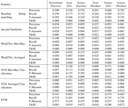
We evaluated the taxonomy extraction procedure in two stages: firstly, we evaluated the results for the individual features using the greedy taxonomy construction procedure as described above. The results for this are given in Table 2, where we present the edge precision, recall and F-Measure based on the number of edges that match those in the tax-onomy we are trying to create. In addition, we present the Fowlkes and Mallows metric (Fowlkes and Mallows, 1983) following the TExEval task as it “measures level by level how well a target taxonomy clusters similar nodes com-pared to a gold standard taxonomy” (Bordea et al., 2016).

In Table 2 the baseline features, Jaccard similarity (Sec-tion 3.3.), and Word2Vec similarities (Sec(Sec-tion 3.4. and 3.5.) are obtained in an unsupervised manner. The supervised re-sults for the SVD and the combination of features with an SVM are also given in this table, where we held out the evaluation dataset and trained on all other datasets.

5. Conclusion

Taxonomy learning is a task that has up until now not achieved satisfactory results. In particular, research on ter-minology extraction using has not produced a higher F-Measure than for a very simple baseline of whether a sub-string is included in the term. While the TExEval results did show that these methods can improve in terms of the Modified Fowlkes and Mallows methods, this metric is very sensitive to the topology of the hierarchy, such as the depth of the network and the average number of children of a node. We present a new method that uses word embed-dings in order to calculate the taxonomic relationship be-tween two concepts in a directed manner. We compare this to the baseline used in the recent TExEval task, and show that while this metric itself does not outperform the base-line, it can easily be combined by means of a SVM classi-fier to produce a model that does outperform the baseline consistently in terms of F-Measure, proving a state-of-the-art result above the results of the TExEval task. While the improvements in F-Measure are significant and show the effectiveness of our methodology, we do not see the same improvements in the Fowlkes and Mallows score suggest-ing that the overall structure of our networks is not as good. This is likely due to the way the network has been con-structed with a greedy algorithm and future work will look into the way that the network is constructed in order to pro-duce a better overall taxonomy.

6. Bibliographical References

Astrakhantsev, N. (2016). ATR4S: Toolkit with state-of-the-art automatic terms recognition methods in scala.

arXiv preprint arXiv:1611.07804.

Bordea, G., Lefever, E., and Buitelaar, P. (2016). SemEval-2016 task 13: Taxonomy extraction evaluation (TExEval-2). InSemEval-2016, pages 1081–1091. As-sociation for Computational Linguistics.

Buitelaar, P., Cimiano, P., and Magnini, B. (2005). Ontol-ogy learning from text: methods, evaluation and appli-cations. IOS press.

Buitelaar, P., Bordea, G., and Polajnar, T. (2013). Domain-independent term extraction through domain modelling. Inthe 10th International Conference on Terminology and Artificial Intelligence (TIA 2013), Paris, France. Cleuziou, G. and Moreno, J. G. (2016). QASSIT at

SemEval-2016 Task 13: On the integration of seman-tic vectors in pretopological spaces for lexical taxonomy acquisition. In10th International Workshop on Semantic Evaluation (SemEval-2016), pages 1315–1319.

Cortes, C. and Vapnik, V. (1995). Support-vector net-works. Machine learning, 20(3):273–297.

Fellbaum, C. (1998).WordNet. John Wiley & Sons, Inc. Fowlkes, E. B. and Mallows, C. L. (1983). A method for

comparing two hierarchical clusterings. Journal of the American statistical association, 78(383):553–569. Fu, R., Guo, J., Qin, B., Che, W., Wang, H., and Liu,

T. (2014). Learning semantic hierarchies via word em-beddings. InProceedings of the 2014 Conference of the Association for Computational Linguistics, pages 1199– 1209.

Gangemi, A., Guarino, N., Masolo, C., Oltramari, A., and Schneider, L. (2002). Sweetening ontologies with DOLCE. Knowledge engineering and knowledge man-agement: Ontologies and the semantic Web, pages 223– 233.

Hearst, M. A. (1992). Automatic acquisition of hyponyms from large text corpora. InProceedings of the 14th con-ference on Computational linguistics-Volume 2, pages 539–545. Association for Computational Linguistics. IEEE. (2017). 2017 IEEE taxonomy. Technical report,

The Institute of Electrical and Electronics Engineers. Kruskal, J. B. (1956). On the shortest spanning subtree of a

graph and the traveling salesman problem. Proceedings of the American Mathematical Society, (7):48–50. Maitra, P. and Das, D. (2016). JUNLP at SemEval-2016

Task 13: A language independent approach for hy-pernym identification. In 10th International Workshop on Semantic Evaluation (SemEval-2016), pages 1310– 1314.

McNemar, Q. (1947). Note on the sampling error of the difference between correlated proportions or percent-ages. Psychometrika, 12(2):153–157.

Mikolov, T., Sutskever, I., Chen, K., Corrado, G. S., and Dean, J. (2013). Distributed representations of words and phrases and their compositionality. In Advances in neural information processing systems, pages 3111– 3119.

(6)

automatic construction, evaluation and application of a wide-coverage multilingual semantic network. Artificial Intelligence, 193:217–250.

Navigli, R., Velardi, P., and Faralli, S. (2011). A graph-based algorithm for inducing lexical taxonomies from scratch. InIJCAI, volume 2, page 2.

Panchenko, A., Faralli, S., Ruppert, E., Remus, S., Naets, H., Fairon, C., Ponzetto, S. P., and Biemann, C. (2016). TAXI at SemEval-2016 Task 13: a taxonomy induction method based on lexico-syntactic patterns, substrings and focused crawling. In 10th International Workshop on Semantic Evaluation (SemEval-2016).

Petersen, K. B., Pedersen, M. S., et al. (2008). The matrix cookbook.Technical University of Denmark, 7(15):510. Shwartz, V., Goldberg, Y., and Dagan, I. (2016). Improving hypernymy detection with an integrated path-based and distributional method. arXiv preprint arXiv:1603.06076.

Tan, L., Bond, F., and van Genabith, J. (2016). USAAR at SemEval-2016 Task 13: Hyponym endocentricity. In10th International Workshop on Semantic Evaluation (SemEval-2016).