IBM Computation Seminar Dec49 pdf

(1)

(2)

PROCEEDINGS

Computation

Seminar

DECEMBER

1949

EDITED BY IBM APPLIED SCIENCE DEPARTMENT CUTHBERT C. HURD,

Director

INTERN ATION AL

BUSINESS

MACHINES

CORPORATION

(3)

P R I N T E D I N T H E

International Business Machines Corporation

590 Madison Avenu(!, New York 22, N. Y. Form 22-8342-0

(4)

FOREWORD

A

COMPUTATION SEMINAR, sponsored by the

Inter-.n

national Business Machines Corporation, was

held in the IBM Department of Education, Endicott,

New York, from December 5 to 9, 1949. Attending the

Seminar were one hundred and seven research engineers

and scientists who are experienced both in applying

mathematical methods to the solution of physical

prob-lems and in the associated punched card methods of

computation. Consequently, these Proceedings represent

a valuable contribution to the computing art. The

Inter-national Business Machines Corporation wishes to

ex-press its appreciation to all those who participated in

(5)

(6)

CONTENTS

The Future of High-Speed Computing

Some Methods of Solving Hyperbolic and Parabolic Partial Differential Equations

Numerical Solution of Partial Differential Equations An Eigenvalue Problem of the Laplace Operator

A Numerical Solution for Systems of Linear Differential

Eq~ations Occu"ing in Problems of Structures

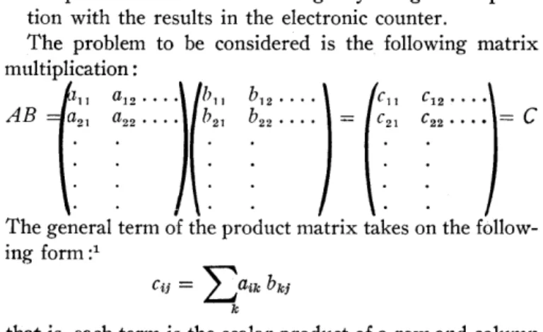
Matrix Methods

Inversion of an Alternant Matrix

Matrix Multiplication on the IBM Card-Programmed Electronic Calculator

Machine Methods for Finding Characteristic Roots of a Matrix

Solution of Simultaneous Linear Algebraic Equations Using the IBM Type 604 ElectronicCa/culating Punch Rational Approximation in High-Speed Computing The Construction of Tables

A Description of Several Optimum Interval Tables Table Interpolation Employing the IBM Type 604

Electronic Ca/Culating Punch

An Algorithm for Fitting a Polynomial through n Given Points

The Monte Carlo Method and Its Applications

A Punched Card Application of the Monte Carlo Method

(presented by EDWARD W. BAILEY)

A Monte Carlo Method of Solving Laplace's Equation

Further Remarks on Stochastic Methods in Quantum Mechanics Standard Methods of AnalyZing Data

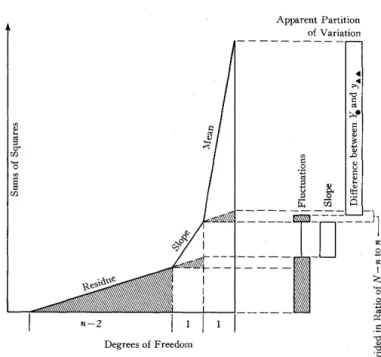
The Applications of Machine Methods to Analysis of Variance and Multiple Regression

-JOHN VON NEUMANN 13

-RICHARD W. HAMMING 14

-EVERETT C. YOWELL. . . • 24

-HARRY H. HUMMEL 29

- P AUL E. BISCH 35

-KAISER S. KUNZ 37

-BONALYN A. LUCKEY

43

-JOHN P. KELLY • . . • . • . •

47

-FRANZ L. ALT

49

-JOHN LOWE.

54

--CECIL HASTINGS, JR.

57

-PAUL HERGET. 62

-STUART L. CROSSMAN

67

-EVERETT KIMBALL, JR.

69

- F . N. FRENKIEL

H. POLACHEK 71

-MARK KAC

M. D. DONSKER •

74

-Po C. JOHNSON

F. C. UFFELMAN 82

-EVERETT C. YOWELL 89

-GILBERT W. KING. 92

-JOHN W. TUKEY .

95

(7)

Transforming Theodolite Data

Minimum Volume Calculations with Many Operations on the IBM Type 604 Electronic Calculating Punch Transition from Problem to Card Program

Best Starting Values for an Iterative Process of Taking Roots Improvement in the Convergence of MethodJ of

Successive Approximation

Single Order Reduction of a Complex Matrix

Simplification of Statistical Computations as Adapted to a Pttnched Card Service Bureau

Forms of Analysis for Either Measurement or

Enumeration Data Amenable to Machine Methods Remarks on the IBM Relay Calculator

An Improved Punched Card Method for Crystal Structure Factor Calculations

The Calculation of Complex Hypergeometric Functions with the IBM T)lpe 602~A Calculating Punch The Calculation of Roots of Complex Polynomials

Using the IBM Type 602-A Calculating Punch Practical Inversion of Matrices of High Order

-HENR Y SCHUTZBERGER 119

-WILLIAM D. BELL . ₁₂₄

-GREGORY

J.

TOBEN 128

-PRESTON C. HAMMER 132

- L. RICHARD TURNER . 135

-RANDALL E. PORTER . 138

- W . T. SOUTHWORTH

J.

E. BACHELDER . . . 141

-A. E. BRANDT ₁₄₉

-MARK LOTKIN. ₁₅₄

-MANDALAY D. GREMS . . . 158

-HARVEY GELLMAN . . . 161

-JOHN LOWE . . . 169

(8)

PARTICIPANTS

ALT, FRANZ L., Associate Chief

Computation Laboratory, National Bureau of Standards Washington, D. C.

ARNOLD, KENNETH J., Assistant Professor of Mathematics University of Wisconsin

Madison, Wisconsin

BAILEY, EDWARD W., Statistician

Y-12 Plant, Carbide and Carbon Chemicals Corporation Oak Ridge, Tennessee

BARBER, E. A.

Engineering Laboratory, IBM Corporation Endicott, New York

BAUER, S. H., Professor of Chemistry Cornell University

Ithaca, New York

BELL, WILLIAM D., Vice-President Telecomputing Corporation

Burbank, California

BELZER, JACK, Mathematician

Cryogenic Laboratory, Ohio State University Columbus, Ohio

BENNETT, CARL A., Statistician General Electric Company

Richland, Washington

BERMAN, JULIAN H., Flutter Analyst Fairchild Aircraft Corporation

Hagerstown, Maryland

BINGHAM, RONALD H., Research Specialist Ansco Division of General Aniline and Film Corporation Binghamton, New York

BISCH, PAUL E., Engineer

In Charge of Special Structures, North American Aviation, Incorporated Los Angeles, California

BRAGG, JOHN, Professor of Chemistry Cornell University

Ithaca, New York

BRANDT, A. E., Biometrician Atomic Energy Commission New York, New York BRILLOUlN, LEON, Director

Electronic Education, IBM Corporation New York, New York

CLARK, H. KENNETH

Department of Pure Science, IBM Corporation New York, New York

CONCORDIA, CHARLES, Engineer General Electric Company Schenectady, New York

COULTER, W. WAYNE, Assistant Director of Research International Chiropractors Association

Davenport, Iowa

CROSSMAN, STUART L., Group Supervisor Computing Laboratory, United Aircraft Corporation East Hartford, Connecticut

CURL, GILBERT H., Senior Physicist Navy Electronics Laboratory

San Diego, California

DISMUKE, NANCY M., Mathematician Oak Ridge National Laboratory

Oak Ridge, Tennessee

DOCKERTY, STUART M., Research Physicist Corning Glass Works

Corning, New York

DUKE, JAMES B., Analytical EnJ!,ineer

Hamilton Standard Division, United Aircraft Corporation East Hartford, Connecticut

DUNCOMBE, RAYNOR L., Astronomer

Nautical Almanac Division, U. S. Naval Observatory Washington, D. C.

DYE, WILLIAM S. III, Supervisor

Tabulating Division, The Pennsylvania State College State College, Pennsylvania

ECKERT, WALLACE J., Director

FERBER, BENJAMIN, Research Engineer Consolidated V ultee Aircraft Corporation San Diego, California

FINLAYSON, L. D., Process Control and Product Engineer Corning Glass Works

Corning, New York

GELLMAN, HARVEY, Staff Mathematician

Computation Centre, McLennan Laboratory, University of Toronto Toronto, Ontario

GOODMAN, L. E., Assistant Professor of Civil Engineering Graduate College, University of Illinois

Urbana, Illinois

GOTLIEB, CALVIN C., Acting Director

Computation Centre, McLennan Laboratory, University of Toronto Toronto, Ontario

GREMS, MANDALAY D., Analytical Engineer General Electric Company

Schenectady, New York

GROSCH, H. R. ]., Senior Staff Member

Watson Scientific Computing Laboratory, IBM Corporation New York, New York

HAMMER, PRESTON C., Staff Member

Los Alamos Scientific Laboratory, University of California Los Alamos, New Mexico

(9)

Watson Scientific Computing Laboratory, IBM Corporation New York, New York

HARDER, EDWIN L., Consulting Transmission Engineer

Westinghouse Electric Company East Pittsburgh, Pennsylvania

HASTINGS, BRIAN T., Project Engineer

Computation Branch, Air Materiel Command Wright Field, Dayton, Ohio

HASTINGS, CECIL JR., Associate Mathematician

The RAND Corporation Santa Monica, California

HEISER, DONALD H., Mathematician

U. S. Naval Proving Ground Dahlgren, Virginia

HENRY, HARRY C., Chief

Office of Air Research, Air Materiel Command, Wright Field Dayton, Ohio

HERGET, PAUL, Director

Cincinnati Observatory, University of Cincinnati Cincinnati, Ohio

HORNER, JOHN T., Project Engineer

Allison Division, General Motors Corporation Indianapolis, Indiana

HUMMEL, HARRY H., Associate Physicist

Argonne National Laboratory Lemont, Illinois

HUNTER,

J.

STUART, Assistant Statistician

University of North Carolina Raleigh, North Carolina

HURD, CUTHBERT C., Director

Applied Science Department, IBM Corporation New York, New York

JOHNSON, PHYLLIS C., Statistician

Y-12 Plant, Carbide and Carbon Chemicals Corporation Oak Ridge, Tennessee .

JOHNSON , WALTER H.

KAC, MARK, Professor of Mathematics

Cornell University Ithaca, New York

KEAST, FRANCIS H., Chief Aerodynamicist

Gas Turbine Division, A. V. Roe, Canada, Limited Malton, Ontario

KELLER, ALLEN

General Electric Company Lynn, Massachusetts

KELLY, JOHN P., Head

Central Statistical Laboratory,

K-25 Plant, Carbide and Carbon Chemicals Corporation Oak Ridge, Tennessee

KIMBALL, EVERETT, JR., Research Associate

Massachusetts Institute of Technology Cambridge, Massachusetts

Arthur D. Little, Incorporated, and Research Laboratory for Electronics Massachusetts Institute of Technology, Cambridge, Massachusetts

KOCH, WARREN B., Aeronautical Engineer

Glenn L. Martin Company Baltimore, Maryland

KRAFT, HANS, Aerodynamicist

Turbine Engineering Division, General Electric Company Schenectady, New York

KRAWITZ, ELEANOR

Watson Scientific Computing Laboratory. IBM Corporation New York, New York

KUNZ, KAISER S., Associate Profeuor of Electrical Engineering

Case Institute of Technology Cleveland, Ohio

LEVIN , JOSEPH

Computation Laboratory, National Bureau of Standards Washington, D. C.

LOTKIN, MARK, Mathematician

Ballistic Research Laboratories, Aberdeen Proving Ground Aberdeen, Maryland

LOWE, JOHN, Staff Assistant

Engineering Tabulating, Douglas Aircraft Company, Incorporated Santa Monica, California

LUCKEY, BONALYN A., Engineering Assistant.

General Electric Company Schenectady, New York

MADDEN, JOHN D., Mathematician

The RAND Corporation Santa Monica, California

MALONEY, CLIFFORD J., Chief

Statistical Branch, Camp Detrick Frederick, Maryland

MARSH, H. WYSOR, JR., Chief Mathematics Consultant

u. S. Navy Underwater Sound Laboratory New London, Connecticut

MCPHERSON, JOHN C., Vice-President

IBM Corporation New YorK, New York

MITCHELL, WILBUR L., Mathematician

Holloman Air Force Base Alamogordo, New Mexico

MONROE, ROBERT J.

Institute of Statistics, University of North Carolina Raleigh, North Carolina

MORRIS, PERCY T., Technical Assistant to the Chief

Statistical Division, U. S. Air Force, Wright Field Dayton, Ohio

MORRISON, WINIFRED

The Texas Company Beacon, New York

MORTON,

J.

E.

(10)

MOSHMAN, JACK, Statistician

u.

S. Atomic Energy Commission Oak Ridge, Tennessee

MYERS, FRANKLIN G., Design Specialist

Glenn L. Martin Company Baltimore, Maryland

PENDERY, DONALD W.

POLACHEK, H., Mathematician

Naval Ordnance Laboratory, White Oak, Silver Springs, Maryland

PORTER, RANDALL E.

Physical Research Unit, Boeing Airplane Company Seattle, Washington

RICE, REX, JR., Research Engineer

Northrop Aircraft Company Hawthorne, California

RICH, KENNETH C., Mathematician

Naval Ordnance Test Station Inyokern, California

RIDER, WILLIAM B.

Applied Science Department, IBM Corporation St. Louis, Missouri

RINALDI, LEONARD D., Mathematician

Cornell Aeronautical Laboratory, Incorporated Buffalo, New York

ROCHESTER, NATHANIEL

Engineering Laboratory, IBM Corporation Poughkeepsie, New York

SAMUEL, ARTHUR L.

Engineering Laboratory, IBM Corporation Poughkeepsie, New York

SCHMIDT, CARL A., JR., IBM Supervisor and Coordinator

Fairchild Engine and Airplane Corporation Hagerstown, Maryland

ScHUMACKER, LLOYD E., Flight Research Engineer

Flight Test Division, Headquarters Air Materiel Command Wright Field, Dayton, Ohio

ScHUTZBERGER, HENRY, Division Leader

Test Data Division, Sandia Corporation Albuquerque, New Mexico

SHELDON, JOHN

SHREVE, DARREL R.

Research Laboratory, The Carter Oil Company Tulsa, Oklahoma

SMITH, ALBERT E., Chemist

Physics Department, Shell Development Corporation Emeryville, California

SMITH, ROBERT W., Mathematician

U. S. Bureau of Mines Pittsburgh, Pennsylvania

SONHEIM, DANIEL W., Research Analyst

Ordnance Aerophysics Laboratory, Consolidated Vultee Aircraft Corporation, Daingerfield, Texas

SOROKA, WALTER W., Associate Professor of Engineering Design

College of Engineering, University of California Berkeley, California

SOUTHWORTH, W. T., Director

Punched Card Applications, The State College of Washington Pullman, Washington

SPENCER, ROBERT S., Research Physicist

Dow Chemical Company Midland, Michigan

STEWART, ELIZABETH A.

STULEN, FOSTER B., Chief Structures Engineer

Propeller Division, Curtiss Wright Corporation Caldwell, New Jersey

THOMPSON, PHILIP M., Physicist

Hanford Works, General Electric Company Richland, Washington

TOBEN, GREGORY j., Supervisor

IBM Group, Northrop Aircraft, Incorporated Hawthorne, California

TUKEY, JOHN W., Associate Professor of Mathematics

Princeton University Princeton, New Jersey

TURNER, L. RICHARD, Coordinator of Computing Techniques

Lewis Flight Propulsion Laboratory, NACA Cleveland, Ohio

VERZUH, FRANK M., Research Associate

Electrical Engineering, Massachusetts Institute of Technology Cambridge, Massachusetts

WAHL, AR'!HUR M., Advisory Engineer

Westinghouse Electric Company Pittsburgh, Pennsylvania

WETMORE, WARREN L., Physicist

Research Laboratory, Corning Glass Works Corning, New York

WHEELER, BYRON W., JR.

Corning Glass Works Corning, New York

WILSON, LEWIS R., JR.

Tabulating Department, Consolidated Vultee Aircraft Corporation Fort Worth, Texas

WOLANSKI, HENRY S., Aerodynamicist

Consolidated Vultee Aircraft Corporation Fort Worth, Texas

WOMBLE, AETNA K.

YORKE, GREGORY B., Statistician

A. V. Roe, Canada, Limited Malton, Ontario

YOWELL, EVERETT C., Mathematician

(11)

(12)

The Future of High-Speed Computing*

JOHN VON NEUMANN

Institute for Advanced Study

A M A

J

0

Reo NeE R N

which is frequently voiced in connection with very fast computing machines, particu-larly in view of the extremely high speeds which may now be hoped for, is that they will do themselves out of busi-ness rapidly; that is, that they will out-run the planning and coding which they require and, therefore, run out of work.

I do not believe that this objection will prove to be valid in actual fact. It is quite true that for problems of those sizes which in the past~and even in the nearest past-have been the normal ones for computing machines, plan-ning and coding required much more time than the actual solution of the problem would require on one of the hoped-for, extremely fast future machines. It must be considered, however, that in these cases the problem-size was dictated by the speed of the computing machines then available. In other words, the size essentially adjusted itself auto-matically so that the problem-solution time became longer, but not prohibitively longer, than the planning and coding time.

For faster machines, the same automatic mechanism will exert pressure toward problems of larger size, and the equilibrium between planning and coding time on one hand, and problem-solution time on the other, will again restore itself on a reasonable level once it will have been really understood how to use these faster machines. This will, of course, take some time. There will be a year or two, perhaps, during which extremely fast machines will have to be used relatively inefficiently while we are finding the right type and size problems for them. I do not be-lieve, however, that this period will be a very long one, and it is likely to be a very interesting and fruitful one. In addition, the problem types which lead to these larger sizes can already now be discerned, even before the extreme machine types to which I refer are available.

Another point deserving mention is this. There will probably arise, together with the large-size problems which

*This is a digest of an address presented at the IBM Seminar on Scientific Computation, November, 1949.

are in "equilibrium" with the speed of the machine, other and smaller, "subliminal" problems, which one may want to do on a fast machine, although the planning and pro-gramming time is longer than the solution time, simply because it is not worthwhile to build a slower machine for smaller problems, after the faster machine for larger problems is already available. It is, however, not these "subliminal" problems, but those of the "right" size which justify the existence and the characteristics of the fast machines.

Some problem classes which are likely to be of the "right" size for fast machines are of the following:

1. In hydrodynamics, problems involving two and three dimensions. In the important field of turbulence, in par-ticular, three-dimensional problems will have to be pri-marily considered.

2. Problems involving the· more difficult parts of com-pressible hydrodynamics, especially shock wave formation and interaction.

3. Problems involving the interaction of hydrodynamics with various forms of chemical or nuclear reaction kinetics.

4. Quantum mechanical wave function determinations -when two or more particles are involved and the prob-lem is, therefore, one of a high dimensionality.

(13)

Some Methods of Solving Hyperholic and Paraholic

Partial Differential Equations

RICHARD

w.

HAMMING

Bell Telefrhone Laboratories

THE M A IN PUR P 0 S

E

of this paper is to present a broad, non-mathematical introduction to the general field of computing the solutions of partial differential equations of the hyperbolic and parabolic types, as well as some re-lated classes of equations. I hope to show that there exist methods for reducing such problems to a form suitable for formal computation, with a reasonable expectation of ar-riving at a usable answer.

I have selected four particular problems to discuss. These have been chosen and arranged to bring out certain points which I feel are important. The first problem is almost trivial as there exist well-known analytical methods for solving it, while the last is a rather complicated partial differential-integral equation for which there is practically no known mathematical theory.

To avoid details, I shall give only a brief introduction to the physical situation from which the equations came. Nor shall I dwell at all on the importance or meaning of the solutions obtained.

Lastly, I have chosen only equations having two inde-pendent variables, usually a space variable and a time variable. Similar methods apply to equations having three and more independent variables.

I have not attempted to define rigorously what is meant by hyperbolic or parabolic partial differential equations, nor shall I later. Instead, I intend to bring out certain common properties, and inferentially these properties de-fine the classes of equations. In fact, from a computer's point of view it is the class of problems which is amenable to the same type of attack that provides the natural classi-fication. It is on this basis that I have included a partial differenial-integral equation as the last example.

Each of the four problems is carried successively further toward its solution until, in the last example, I have given the detailed steps which were actually used.

If, in the rest of the paper, I do not mention any names" it should not be inferred that I did everything alone; on the contrary, I have at times played but a minor part in the entire effort.

14

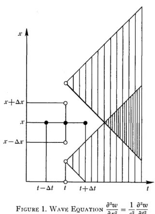
THE WAVE EQUATION

The classic and best known example of a hyperbolic partial differential equation in two independent variables is the wave equation:

a

2_w ₁

a

2_w

ax

2 - _c2

at

2 _•

This is the equation which describes the propagation of signals, w) in one dimension, x. The signals progress in time, t) with a velocity, c. This equation is a linear equation and, as such, there is a large body of theory available for use in solving it. Thus, it is not likely that anyone would be called upon to solve it numerically except in very un-usual circumstances. Nevertheless, I have chosen it as my first example, since I hope its simplicity and familiarity to you will aid in bringing out the main points I wish to make. In solving partial differential equations it is customary to replace the given equations with corresponding differ-ence equations, and then to solve these differdiffer-ence equa-tions. Whether one looks at the approximation as being made once and for all and then solving the difference equations as exactly as possible, or whether one looks at the difference equations as being an approximation at every stage is a matter of viewpoint only. I personally tend to the latter view.

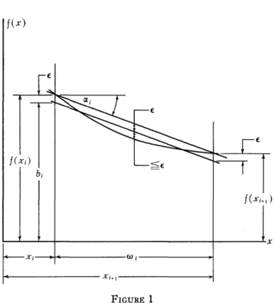
In the case at hand, the second differences are clearly used as approximations to the second derivatives. Such a choice immediately dictates an equally spaced rectangular net of points at which the problem is to be solved. Such a net is shown in Figure 1. The space coordinate, x) is ver-tical while the time coordinate, t) is horizontal. Thus, at a fixed time, t) we look along the corresponding vertical line to see what the solution is in space, %.

(14)

S E MI.N A R

/ /

~

/

/ /

/

~,

"

~t

,

/

V

~:

~

t-b.t

a

2_w ₁

a

2_w

FIGURE 1. WAV}<~ EQUATION ~

=

9"--;---9

uX- c-

ut-called the "cone of disturbance." The slopes of the bound-ing lines indicate the velocity of propagation c~ and in this simple case they are straight lines. In the mathematical theory of partial differential equations the lines are called "characteristics. "

The figure shows a second disturbance started at the same time, t, but at a lower point. This, too, spreads out as time goes on, and there finally occurs a time when the two cones overlap.

Consider, again, the given equation. The second differ-ence in the x direction is calculated from the three points which are connected by the vertical line. This is to be equated to 1/ c2 _{times the second difference in the time}

direction, which naturally uses the three solid black points. Suppose that the solution of the problem, up to the time t,

is known, then we have an equation giving an estimate of the solution at one point at a later time, t

+

6.t.

Suppose, now, that the spacing in the x direction is kept as before, but the spacing in t is increased so as to predict as far as possible into the future. It should be obvious that the spacing in t cannot increase so far that the advanced point falls into the cones of disturbance of the first two points which are neglected. To do so is to neglect effects that could clearly alter the estimate of what is going to happen at such a point. Thus, it is found that, for a given spacing in the x direction, and a formula of a given span for esti-mating derivatives in the x direction, there is a maximum

15

permissible spacing in the t direction, beyond which it is impossible to go and still expect any reasonable answer. In this simple case the condition may be written

6.t

<

6.x .

- c

Supposing that this condition has been satisfied, and also, the solution up to some time t is known, the above method may be used to advance the solution a distance

6.t

at all interior points. A point on the boundary cannot be so advanced. There must be independent information as to what is happening on the boundary. Such conditions are called "boundary conditions" and are usually given with the problem. The simplest kind of -boundary condition gives the values of the dependent variable w by means of a definite formula. More complex situations may give only a combination of a function wand its derivative dw/ dx.

Such situations may require special handling when solving the problem in a computing machine, but in principle are straightforward.

A step forward at all points x is usually called a "cycle," and the solution of a problem consists of many, many repetitions of the basic cycle. The sole remaining question is that of starting the solution for the first cycle or two. Just as in the case of ordinary differential equations, this usually requires special handling and is based on some simple Taylor's series expansion of the solution. In prac-tice, this step is often done by hand before the problem is put onto whatever machines are available.

As remarked before, this problem -is not realistic, so having made a few points about spacing, boundary condi-tions, and initial, or starting, condicondi-tions, let us turn to a more complex problem.

THE Two-BEAM TUBE

The two-beam tube is a tube with two electron beams going down the length of it together. Upon one beam of electrons a signal is imposed. The second beam, which has a slightly greater velocity, interacts with the first beam through their electric fields, and may be regarded as giving up some of its energy to the first beam. This in turn pro-duces, one hopes, an amplification of the signal on the first beam.

The equations describing one particular idealization of such a tube are:

a:

ti

+

a~

_(PiVi)

=

₀

l

i = 1,2

aVi

a

+

at

+

Vi

ax (

Vi) =

2"

~!

= k2q,

+

(PI

+

P2)

(15)

where the solution is to be periodic in time of period 1,

and we are given information as to the state of affairs at the beginning of the tube, Z

=

O. The upper two equations

for i = 1 describe one of the beams, while for i = 2 they describe the other beam. The lower two equations describe the interaction between the two beams of electrons.

I shall gloss over any questions of existence theorems for such a system and merely suppose that there is a solu-tion. The information needed to start the problem at X' = 0 comes from the" linear" theory which is not hard to find from a "linearized" form of the equations. We are here called upon to calculate the essentially nonlinear aspects of the tube.

The first reduction of the equations has already been performed before they were written as above, namely, that of transforming out of the equations all of the various constants and parameters of the problem that we could. 1n their present state the Vi of the equations give the

ve-locities of the two beams measured in units of the mean velocity, the Pi the corresponding charge densities of the beams measured in mean charge density units, while the

cp and 'i1 describe the electric field in suitable dimension-less units.

Since we are expecting a "wave-like" solution, it is convenient to transform to a moving coordinate system which moves with the expected mean velocity of the two beams. In such a coordinate system, the dependent vari-ables Pi, Vi, CP and 'i1 may be expected to change slowly.

The equations obtained by such a transformation,

are

or

T=t-X'

a

aO"

[PiVi]

=

aT

[pi (Vi - 1)]

a

aO"

[Vi

2]

=

aT

[(Vi - 1)2]

+

'i1

aw _ aW

2

aO" -

a:;

+

(Pt

+

P2)

+

k CP acp acp

aO"

=

a;

+

'i1 ,

where the solution is still periodic in time T with period 1.

In solving the usual hyperbolic type of equation, one advances step by step in time, but in this problem a pe-riodic condition in time is given on the solution, and were the time to be advanced, it would be difficult to make the solution come out periodic. There would also be difficulty in finding suitable starting conditions. Instead of advancing in time, advancement is step by step down the length of the tube in the 0" direction, using the periodic condition in

T to help estimate the derivatives in the T direction at the

ends of the interval. Thus, the periodic condition in effect supplies the boundary conditions.

One may calculate, if one wishes, the characteristic lines and determine the cones of disturbance, but in this case it must be looked at sidewise, as it were. Assuming that the solution is known for an interval of time, how far in space may the solution be predicted at a time corresponding to the mid-point of the time interval? If the cones of disturb-ance were to be calctflated, it would be found, as is usual in nonlinear problems, that the velocity of propagation de-pends on the solution which is to be calculated. For exam-ple, a large shock wave of an explosion travels at a velocity that depends not only on the medium through which it passes, but also upon the amplitude of the shock wave itself. Let us turn to the question of choosing a net of points at which we shall try to calculate an approximate solution. The use of a two-point formula in the T direction for

esti-mating the T derivativ~s requires a great many points and

produces a very fine spacing in the 0" direction. If a

four-point formula is chosen (a three-four-point one is hardly better than a two-point one for estimating first derivatives), the following is obtained,

~'(O) _ f( -3/2) - 27f( -1/2) +27f( 1/2) - f(3/2)

J - 24 L}. T

+

€ ,

with an error term of the order of

3

€,-..; 640 (L}.T)4f(V) (8)

A formula like this is easiest to obtain by expanding each term about the mid-point of the interval in a Taylor's series with ~ remainder. Since in this moving coordinate system we expect a sinusoidal variation in time, the fifth derivative is estimated from the function

f

= sin 271'T •

In order to obtain an accuracy of about 1 part in 104 _as

the maximum error, it is necessary to choose 24 points in the T direction-a most fortunate choice in view of the

product 24L}.T in the denominator of the estimate. The statement that the maximum error at anyone point is at most one part in 104 _{tells very little about the}

accu-mulated error due to many, many small errors, but as far as I know, there are no general methods which are both practical and close enough to help out in this type of situ-ation. My solution to this dilemma is twofold:

1. To the person who proposed the problem, I pose questions such as, "If the solution is disturbed at a given point, will it tend to grow, remain the same, or die out?" At the same time, I try to ariswer the question independently, keeping an eye on the rou-tine to be used in the solution of the problem. 2. Hope that a properly posed problem does have a

solution, and that human ingenuity is adequate to the problem at hand.

(16)

S E M I N A R

(1

o x

x o

3/2

--:---1

1/2

---~

---1

0 - - - x ;

-1/2

--:---]

-3/2

--0---x 0

0 x

x; 0

-r-/::'-r -r

o

p and Vi known x""'- at x points

o'+-<I> and

*

known at 0 pomts x

o K

o x o x

o

f' (0) = f( - 3/2) - 27f( -1/2) 24(/::'%)

+

27f( 1/2) - f( 3/2)

+

f

where f " ' " ~ (/::'x) 4j(V) (8)

640

FIGURE 2

inactivity. One should, of course, make a diligent effort to resolve this dilemma, but pending that time, go ahead and hOope for the best, ready at any time to suspect the solu-tions obtained.

Returning to our problem, some Oof the advantages of a four-point' formula for estimating the derivatives in the

7'

direction have been listed. Let us look at the disadvantages in general. In the first place, except in periodic cases such as this one, where one can double back the solution from the top of the interval to add on to the bottom, the difficult problem of estimating derivatives near the boundaries arises. In the second place, one faces the task of assem-bling information from four different points to estimate the derivative at anyone point. If, for example, the four values lie on four different IBM cards, it is not easy to get the information together. One method would be to calculate both 1 and 27 times the value of the function on each card and then on one pass through the accounting machine-summary punch equipment, using selectors and four counters tOo accumulate the running sums, punch out the proper totals along with suitable identification on each summary punched card.

17

To estimate the derivatives on the (1' direction to advance

one step, a simple two-point formula is used. Since both the four- and two-point formulas give estimates at the mid-points of the intervals, one is led to a "shifting net" of points as shown in Figure 2. Such a net leads to some slight troubles in the identification of points, but gives probably the least calculation where it is necessary to deal with many odd order derivatives. At least in this case, it certainly does. I have glossed over the accuracy of the estimate of the derivative in the (1' direction, but in this

case it was adequate, due to the fineness in the spacing necessary to satisfy the net spacing condition in 6 ( 1 ' and

67'.

Let us drop this problem at this point and take up the next example.

A PARABOLIC PARTIAL DIFFERENTIAL EQUATION

The most common parabolic partial differential equation in two independent variables has the form

dB _ 4rry d2_H

at - c2 a%2 •

Such an equation describes the flow of heat, the diffusion of material, and the magnetization of iron.

In the particular case we shall discuss, a thin slab of permalloy is given, 2 mils thick and of infinite extent in the other two directions. This slab is subjected to an ex-ternal field H which is changing in a sinusoidal fashion with frequency

f.

The question posed is that of determin-ing the frequency of the external field such that B at the center of the slab rises to 90 per cent of its maximum possible value.

I would like to digress here for a moment to remark that it appears to me to be frequently the case that one is asked to determine a constant in the boundary conditions, or a parameter of the problem, such that the solution will have a given form. This is often a way of measuring a physical constant; indeed, when one finds a problem whose solution is sensitive to some parameter, then this may well provide a way of measuring that quantity with a high degree of precision.

Returning to the problem, it is immediately noted that in heat flow or diffusion there is no concept of velocity of propagation; hence the ideas of characteristics and cones of disturbance are of little help. Nevertheless, there is a condition on the spacing in % and t. To arrive at a

neces-sary condition, suppose that at some point an error £ in H

is committed1 due, perhaps, to roundoff. This produces in

turn an error of 2£ in the second difference. Following this through it is found that there is an error of

(17)

in the estimate of B'!;1I2, since a difference equation of the form

Bi+1I2 = Bi-l/2

+

c 2

6. t 1\ 2 Hi

n n 4,ry (

6.% )

2 ~ n

is used. When the value of B is extrapolated to the point

B'!;l for the next cycle the error becomes

c26.t

4,ry(6.%)2 ·3£ .

Using this to calculate the new H of the next cycle, it is found, on expanding in a Taylor's series and keeping only two terms,

I f the original error £ is to produce an effect in the next

cycle at the same point that is not greater than itself, then the following condition must be met,

At < 4,ry(6.X)2 dB

~ = 3c2 _dH'

This condition differs from that of hyperbolic equations in that it depends on the square of 6.x. Thus, if the spac-ing in 6.x is halved, the 6.t must be divided by 4. This is typical of parabolic equations. The inequality takes care of a single roundoff, while if a roundoff at each point is assumed, an additional factor of 7/10 is needed on the right-hand side.

B

H

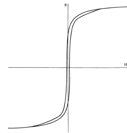
FIGURE 3. HYSTERESIS Loop, MOLYBDENUM PERMALLOY

This condition is clearly necessary in order to expect anything like a reasonable solution; its sufficiency will be discussed later. Note the derivative dB / dH on the right-hand side.

The particular sample of permalloy discussed had a

B-H curve, as shown in Figure 3. Recalling the importance of the derivative dB / dH in the net spacing condition, it is seen that as the problem progresses a very tight spacing must be accepted throughout the problem or else the spacing at various stages must be modified to take advantage of those places where the derivative is large. The latter was chosen.

In the early stages of the computation, while an attempt was made'to obtain an idea of the order of magnitude of the frequency

f,

a crude subdivision of the slab into four zones marked by five points was made. By symmetry one half could be ignored so that, in fact, only three points needed to be followed. The outer point was driven by the boundary condition, while the two inner points followed according to the difference equations.

To test the method, first a B-H curve was used which was a straight line. The comparison with the analytical solution was excellent. To show the reality of the net spacing condition the· problem was deliberately allowed to run past a point where the net should have been tightened. The results are shown in Figure 4. This oscillation is typi-cal of what happens when a net spacing condition is vio-lated, although sometimes it takes the form of a sudden exponential growth instead. Indeed, when such phenomena occur, one may look for a violation of some net spacing condition.

I have emphasized that the condition just derived is a necessary condition. There has been a lot of discussion lately as to whether this is a sufficient condition. Unfor-tunately, I do not have time here to go into this matter more fully. Instead, let me present some of the results obtained several years ago when we did this problem. Figures 5, 6, and 7 show a smooth transition on the solution as the frequency

f

was changed. Any errors are clearly systematic. The jumps in the inner points are due both to the shape of the B-H curve and the extremely coarse spacing of three points. When a finer spacing of five points was used (eight sections of the slab instead of four), much the same picture was found. The labor, of course, was eight times as much since there were twice as many points, and the

6.

t was decreased by a factor of four. This crude spacing should indicate how much valu-able information may be obtained from even the simplest calculations when coupled with a little imagination and insight into the computation.

(18)

H

- 1.0 - 1.1

- 1.2

- 1.3

- 1.4 - 1.5 - 1.6

-1.7

- 1.8

- 1.9

- 2.0

H 20

16

12

08

04

o

04

08

12

16

20

28

f\

o

-MO- Pp ~ ₂ MIL TAPE

f = 18 X 105

2 INTERVAL

Ho

A

~\

IH

.IT

I-i c;

-::;~/

~!x7

X

v

\

--

-

\

~

'><.../ v v V

V

~

---

HI

---

~

- ---

.:..

--;;;:.=

=-T X 108

3 6 40 44 48 52 60 64

FIGURE 4

MO- Py , 1.. _zMIL TAPE

f

=

105

2 INT E RVA L

17

~

/

V

~

10

:/

,/' _~

I

HO _

)

~

/

V

---

~~

T X 108

50 100 150 200 250 300 350 400 500

(19)

H

2.0

1.6 1.2 0.6

0.4

o

- 0.4

- 0.6

- 1.2

~

f = 1.8 X 105

2 INTERVAL

/

~

/

V

/"

/

V

_J

V

v----~

,

~~

V

- 1.6 - 2.0

H

2.0

1.6 1.2 0.8

o 40 60 120

flAo-Py ,

+

~AIL lAPE

f=25X105

2 I NTE RVAL

/

V

T X 106

160 200 240 260

FIGURE 6

/ -

i - - H2

~

HI

l\

r--H2

~

HI

/r

HJ

320

o

V

H

~

/

~ 0

/

rv

0.4

/!/

V--~

/

V~

-0.4

-0.8

-1.2 -1.6 - 2.0

T X 108

o 40 80 120 160 200 240 280 320

FIGURE

7

20

(20)

S E M I N A R

consult not one but a family Oof B-H curves, the one chosen for each point depending on its maximum saturation. This refinement was nOot included in the results shown before, and in any case it produces only a small effect.

THE TRAVELING WAVE TUBE

The last example I wish to consider is that of the travel-ing wave tube. A traveltravel-ing wave tube consists Oof a helix of wire wound around an evacuated cylinder. The pitch of the helix reduces the effective velocity of the field due to an impressed electric current in the helix to around 1/10

that of light. Inside the helix is a beam of electrons going at a velocity slightly greater than the electromagnetic wave frOom the helix. As in the two-beam tube, the stream of electrons interacts with the field and gives up some of its energy to magnify the signal impressed on the helix.

The equations describing one particular idealization of such a tube are

d~~)

= _

Lf2"

sin </>(9, y)d9

1

f21T

'YJ(y),

= -

27rEA(y) 0 cos cf>(O,y)dO

a~

q(O, y)

=

A(:V) sin cf>(O, y)

a

ay cf>(O, y)

=

k

+

'YJ(Y)

+

2Eq(O, y) .

These equations have already been transformed over to a coordinate system mOoving with the wave. The y coordinate measures, in a sense, the length down the tube, while the

°

measures the time.

I f the equations are examined more closely, it is seen that, for each 0, the lower two equations must be solved in order to move the solution Oof q and cf> one step down the tube in the y direction. The sine and cosine of cf> are then summed to obtain numbers depending on the funda-mental frequency. The higher harmonics are clearly being neglected. These upper equations in turn supply the co-efficients for the lower equations. This neglect of the higher harmonics was justified on the physical grounds that the helix damped them out very strongly. As a check, the amount of the second, third, fourth, and fifth har-monics in the beam was calculated later, and it was found that they could indeed be neglected.

The first step is to make a transformatiOon so that the parameters E and k drop out of the equations.

Proceeding much as in the two-beam tube, it was de-cided that 16 points would provide an adequate picture in the

°

direction. Thus, there are 16 pairs of equations like the lower ones to solve. In addition, it was desired to

21

solve eight such problems for different parameter values (which appear in the initial conditions and enter in the "linear" solution used to start the nonlinear problems). This gives 128 pairs of equations to be solved at each cycle, a situation very suitable for IBM equipment. On the other hand, the upper two equations only occur once per problem, or eight times in all, which makes them un-suitable for machine solution. Thus, the solution of the lower equations and calculation of the sums corresponding to the integrals of the upper equations were accomplished on IBM machines, while the rest of the upper equations were solved by hand calculations. Included in the hand calculations was a running check that may be found by integrating the equations over a period and finding the ordinary equations that govern the mean values.

With a spacing chosen in one variable, how is the spac-ing to be chosen in the other? In this case, there is no theory of characteristics, in fact, very little mathematical theory available at all. The obvious was done. A number of spacings were tried, with a crude net space in

60,

and the maximum permissible

6y,

at that stage of the problem, was determined experimentally. Then a spacing

6y

was chosen, comfortably below this limit, although not so far as to make too much work, and the calculation started with the hope that this would either be adequate for the entire problem or that the effect would show up in a no-ticeable manner in the computations. No obvious anomalies appeared; so presumably the spacing of 1/10 unit in y was adequate. The net chosen was rectangular with every other y value being used to calculate the cf> and q, while at the other values the A and 'I] were evaluated. This produces central difference formulas which are the most accurate. The old cycle in cf> -and q- was labeled by a -, the current

values of AO and '1]0 by a 0, and the predicted values of cf>+

and q+ by a

+.

The new values of A++ and '1]++ were labeled

++.

To set up a system of difference equations corresponding to the lower equations: first, an estimate of q+ was ob-tained, then this was used to find a reliable value of cf> + ;

finally, using this cf>+, a better estimate of q+ was obtained. The difference equations describing this situation are

1 ( A O . )

cf>+=</>-+1O .'I]°+q-+1Osm

cf>-AO ( . . )

q+ = q-

+

10 sm cf>- + sm cf>+

L

= ~ sin cf>+

M = ~ q+ sin cf>+

N = ~ cos cf>+ •

The difference equations corresponding to the upper equa-tions have not been shown, but it has been indicated that the solution of both equations was made to depend on three sums labeled LJ M J and N.

(21)

at every fourth decigrade. The advantage of such a unit is that the integral part of the angle automatically gives the number of rotations, and the fractional part gives the value at which to enter the table.

Consider the basic cycle of computation. It is obvious that the accounting machine-summary punch will be best adapted to the summing of the quantities leading to L, M,

and N. This is the natural point to start a cycle, since the cards from the summary punch will have the minimum -amount of information, leaving the rest of the space on the cards for future calculations. These cards will be called detail cards.

Each detail card needs to be identified uniquely. To do this the problem number, the card number which is its () value, and the cycle number which is its y value, are given. The information that the detail cards must carry at this stage to describe the problem is the current values of

cp-and q-. In addition, it is convenient to have the value of the sine of the old angle, sin

cp-.

The master, or rate, cards-the information for which comes from the hand calculations-must have identification consisting of the problem number and the cycle number, and the values of the two dependent variables A

°

and 'YJ0• The

procedure is :

1. Key punch the eight master cards and sort them into their appropriate places, a matter of one sort on one column.

2. Multiply with crossfooting to obtain the quantity,

AO

q+(estimate) - '

10

sin

cp-

+

q- , which is an estimate of the q at the neW cycle.

3. Another multiplier-crossfoot operation produces

°

AO.

q-cp+

=

cp-

+

io

+

100 sm

cp-

+

10

which is the new value of

cp

+. Now the sine and cosine of

cp

must be found.

4. Sort on

cp

for three digits,

5. Collate in the table values of the trigonometric functions,

6. and 7. Using the multiplier, linearly interpolate the values of sine and cosine of

cpo

Each may be obtained with a single pass through the multiplier, provided there are only five figures in the table values and three in their first dif-ferences. The algebraic signs may be picked up from the master cards and held up for the detail cards which fol-low, so that with a suitable complement punching circuit the value and its algebraic sign may be punched.

8. Collate again to remove the table cards and at the same time put the table back in proper order. (Inciden-tally, the same control panel is used for both operations on the collator.)

9. Resort the detail cards so that they are again in order, both as to -the card number and the problem num-ber, a matter of a three-column sort.

10. Multiply-crossfoot to obtain the new value of q from the formula

AO ( .

+. ')

q+

=

q-

+ -

sm

cp-

sm cpT

10

11. Multiply to obtain

q+

sin

cp+.

12. List the calculated values, the three sums L, M, and

N, and summary punch the cards for the next cycle. If these operations are gathered together, it is found that there are 6 passes through a 601 type multiplier, three sorts for a total of

7

columns, two passes through the col-lator, a key punching of 8 cards, and one pass through an accounting machine-summary punch for each cycle.

We used our own accounting department machines with a 601 multiplier modified to have sign control, and three selectors. We operated only at times when they were not doing their main task of getting out the pay checks! N eed-less to say, no arguments ever arose as to priority on the use of the machines.

CONCLUSION

Let me summarize the points I hope I have made. First and foremost, there is a large class of problems where the relative size of the net spacing chosen is of fundamental importance. Where there is no known mathematical the-ory, or where one is ignorant of it, one may still proceed on an experimental basis and watch for either violent oscillations or sudden exponential growths to indicate where the going is not safe.

Second, it is not hard to set up a method of computation for a given problem, and one can estimate the accuracy at any step by some such device as using a Taylor's expansion with a remainder. The harder problem of propagation and compounding of errors I have not answered at all defi-nitely, but have suggested that prudence, physical intuition, and faith will provide one with a suitable guide.

(22)

S E M I N A R

DISCUSSION

Dr. Hammer: The choosing of networks in comparison

to the interval of the variables sometimes can be avoided by using a different system of integration; that is, an im-plicit calculation in which perhaps some of the variables are first found by explicit integration, and then they are recalculated.

Dr. Hamming: You are thinking of the Riemann

method, no doubt, or the von Neumann method of getting a difference equation which involves the present values and simply adjacent values one cycle forward.

Dr. Hammer: Yes. One essentially calculates all the

values at the same time, and then the condition you men-tioned can be violated to some extent.

Dr. Herget: The graphical way in which you portray

the effect of (6. t) 2 to 6.% is very good, and I think it has

been stated in some of these meetings before that to be safe for the convergence involved in this process,

6.t

should be about half of 6.%. Isn't that right?

Dr. Hamming: You can't say any 6.% and

6.t.

It

de-pends on the scale of the variables used. If the variable is multiplied by 10, the spacing would be changed numeri-cally. The condition is stated in terms of the velocity of propagation of signal in the hyperbolic case, and in the parabolic case one considers the derivative dB / dH.

Dr. Grosch: I would like to ask a question about the

nature of the oscillations encountered when the condition is violated. Have you made any effort to see, if you will pardon a nontechnical term, what the mean curve through those oscillations does? Does it follow the solution?

23

Dr. Hamming: Yes, it does.

Dr. Grosch: That is an interesting point.

Dr. Hamming: I f you examine Figure 4, you can see

this is true.

Dr. Grosch: We had a situation like that arise back in

1946 when we were using 601's, and in our case the con-dition on the very short 6.% and

6.t

was not a simple constant but a sort of variable of the column. We had this oscillation happen just a few % intervals from the end; we

tried a fudging method of this sort, and it seemed to work out all right.

Dr. Alt: I think the situation concerning propagation of

the local errors is not as hopeless as you indicate. One can use Green's function in order to study the propagation of errors whenever Green's function is available. If it is not in there, at least one can try to linearize it. We have tried that in a nonlinear problem, too, and it worked out. It can be done. I felt that the problem was simple enough that one didn't even consider publishing it, because it was just a straightforward application of the Green's function.

Dr. Hamming: I agree with what you say completely if

(23)

Numerical Solution of Partial Differential Equations

EVERETT C. YOWELL

National Bureau of Standards

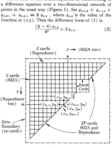
THE US U A L MET HOD S for determining numeri-cal solutions of partial differential equations with specified boundary conditions are based on the approximation of the differential equation by a difference equation. In the case of the two-dimensional Laplace's equation, which is the only one I will speak of today, the differential

equation is a

2

Z

+

aa

2Z

=

o.

The standard approximation is

a%-

Y-~2xf

+

/:}yf 0 h 1\2f' h d d'ff

(~%)2 (~y)2

=

were Dx IS t e secon 1 erence in the % direction and ~~f is the second difference in the y direction.

The exact relation between the differential operator and the difference operator is an infinite series in the difference operator,

a

2f

+

a

2f _ 1 (/::/f 1 1::/f 1 66

f

)

a.r2 ay2 - (6%) 2 !lJ -

12

x

+

90 x - .••

+

(~y)2 (~2yf

- }12 64yf

+

~ ~~f

- ... ) and the standard approximation amouhts to cutting off this series after the first term in % and in y. If only second

differences are to be used, it is obviously advisable that the interval ~% should be chosen sufficiently small so that the term

1~

(

~~

2 becomes negligible. I f this leads to too

small an interval, we try to recover the accuracy by in-cluding more terms of the series in the approximation. The validity of this procedure needs rigorous justification, but it presents a practical computational approach.

N ow differences are linear relations between function values at adjacent points. Hence, any method which works basically on the difference equation will be a method deal-ing with values of the function at specified points within the boundaries. These points are generally chosen sys-tematically to cover the interior of the region with a regu-lar grid. We .shall consider only a square grid, as it is more easily adapted to machine computations than are the tri-angular or hexagonal grids.

The direct approach to the problem is to write out the difference equation for each point of the grid. Since we are dealing with a square grid, ~%

=

~y, we shall call

24

this mesh distance h. Then the difference equation at the point %

=

%i, Y

=

Yj will become:

1

h2 [f(%i-l,Yj) - 2f(%i,Yj)

+

f(%i+l1Yj)

or symbolically

1

h2

+f(%i,Yj-l) - 2f( %i,Yj)

+

f(%i,Yj+l)]

=

0

=0

There is one such equation for each point of the grid. Each equation may involve only interior points, or interior points and boundary points. I f the boundary points are considered as known and transferred to the right sides of the equations in which they occur, then there is a system of n equations, one for each grid point, involving n un-knowns, the values of the function at each grid point, which completely defines the function at the grid points within the boundary. In the present case, it can easily be shown that a unique solution of these equations always exists.

There is one great drawback to this approach to the numerical solution of a differential equation, and that is the number of equations in the system. Consider a rela-tively simple heat conduction problem. \Ve have a cube,

}O cm. on each edge, at a uniform temperature of O°C.

(24)

S E M I N A R

was designed to show how rapidly the number of equa-tions can increase, and is not the type of problem that would be solved in practice, problems of the same order of magnitude are available in the physically interesting problems whose solutions are being sought today.

A second method of attack is the relaxation method of Sir Richard Southwell. Here one guesses at the value of the function at each grid point and then systematically improves the guess. The values of the function are substi-tuted into Laplace's difference equation, and the result will in general differ from zero. This difference, or residual, is computed for each grid point. The largest re-sidual in the entire field is now located, and the value of the function at that point altered in such a way that the residual becomes zero. This is equivalent to adding one quarter of the residual to the residual at each of the four adjacent points, leaving the rest of the field unaffected. The field is again scanned for the largest residual, and it is reduced to zero by changing the value of the function at that point. The process is continued until all the re-siduals become small, one or two units in the last place.

As a hand computing method, relaxation has many ad-vantages. It deals with only a few points at a time, it in-volves very simple operations, and it converges to the solution of the difference equation rather rapidly. And there are variations-over-relaxing and under-relaxing, group relaxing and block relaxing-which increase the speed of convergence. As a machine method, many of these advantages are lost. The speed of convergence de-pends on relaxing the largest residual at each step. Hence, the entire residual field must be scanned before each oper-ation to locate this largest residual. This scanning for size is still a very inefficient operation, particularly when it is interposed between every set of five additions. Then, too, the block and group relaxations, which so speed up the convergence in hand computing, are very difficult to apply using automatic computing machinery.

Another method related to the relaxation method is Liebmann's smoothing method. Once again, we start with the basic difference formula

b

[f(Xi-nY,i)

+

f(Xi+vYj)

+

f(Xi,Yj-l)

+f(Xi,Yj+1) - 4f(Xi,Yj)]

=

O.

If now we multiply the equation by h2 _{and then transfer}

4f(Xi,Yj) to the right-hand side, we have an equation

de-fining f(Xi,YJ) in terms of the four adjacent values of the

function. The method consists in guessing the value of the function at each grid point, and then applying the smooth-ing formula to each point of the grid. The entire field is smoothed again and again until no changes are introduced in the function values to the degree of accuracy required. This method has some advantages and some disadvan-tages. Its main disadvantage is its slow speed of con-vergence. Its advantages are that it deals with only a few

25

points at a time, that it involves only simple operations, and it is adaptable to machine computations. M. Karmes, of New York City, has done this, reporting in 1943 on an adaptation of this method to 601 multipliers. His machine method is straightforward, one quarter of the value of the function at the four neighboring points being summed to give the value at the central point. To assemble correctly the cards to be summed, Karmes prepares four decks of work cards. Each of these contain

if

(Xi,}'j) , but they differ

in that a second argument is introduced in each deck. One contains (i - 1,j); one, (i

+

1,j) ; one, (i,j - 1); and one, (i,j

+

1). The four decks are now sorted together on the second argument and summed, summary punching the new value of the function at each grid point. The deck with the new function values is then reproduced four times, the second arguments are put in, and the process is repeated. This cycle is continued until 'the function values converge within the required accuracy.

A method simil'ar to Liebmann's method, but better adapted to machine computation, has been devised by Dr. Milne and tested on the 604 electronic calculators at the Institute for Numerical Analysis. Dr. Milne was seek-ing to avoid the sortseek-ing problem that led Karmes to the use of four decks of cards. He added two difference oper-ators, each satisfying Laplace's difference equation, to-gether. The first is the usual

=

0,

while the second 1S basically the same operators rotated

45°,

=0

Multiplying each by four and summing, we obtain

1

(25)

The trick now is to multiply through by h2 _{and then add}

36!(%i,Yj) to both sides of the equation. This gives

This equation is now factorable, and we can define two operators U and V such that

1

U !(Xi,Yi)

=

6[!(Zi-l'Yi)

+

4!(%i,Yi)

+

j(%i+l/Yj)]

1

V!(%i,Yi) = 6[f(%i,Yj-l)

+

4!(%i,Yi)

+

!(%i,Yj+l)]O

If these are applied successively to the nth approximation

to the function values at the grid points, they will yield the n

+

1st _{approximation. Or,}

r+l(%i,yj)

=

uv!n(%i,Yj)

=

VU jn(%i,Yi)'

The last equation indicates that the operators commute and that rows or columns may be smoothed first.

This method works nicely on the 604 electronic calculat-ing punch. For each iteration, the cards must be fed through the machine twice, once in row sort and once in column sort. At the end of the second run, a new set of function values will have been computed for each grid point.

The example tested a 9 x 10 rectangular grid with values of arctan % / Y given along the boundaries. \Ve have

avail-able 10 place values of arctan %/y, so that a check was pos-sible on the speed of convergence. The smoothing was ap-plied first by rows and then by columns, although this choice was completely arbitrary.

The wiring of the 604 control panel was simple and straightforward. The value of the function was read into factor storage 3 and 4, and a 4 and a 6 were emitted into the MQ and factor storage 2, respectively, on the read cycle. The analysis chart reads as shown below:

The result 0 f this operation is to punch V

!

(% i,Y j-l) on the

(i,j) card. The two last transfers set up the operation for the next point. This arrangement of storage units will handle any size numbers up to eight digits, and that should include all problems of practical interest today. There is no question of the function values growing too large, as the maximum and minimum values must occur on the boundary.

The wiring of the 521 control panel is a little more com-plicated, as it was desirable to make the control panel auto-matically change itself for the differences between the first and second runs. There are two problems that must be handled on the 521 control panel. The first is that the input fi