Tagging with Hidden Markov Models Using Ambiguous Tags
Alexis Nasr
LaTTice - Universit´e Paris 7
Fr´ed´eric B´echet Laboratoire d’Informatique
d’Avignon
Alexandra Volanschi LaTTice - Universit´e Paris 7
Abstract
Part of speech taggers based on Hidden Markov Models rely on a series of hypothe-ses which make certain errors inevitable. The idea developed in this paper consists in allowing a limited, controlled ambiguity in the output of the tagger in order to avoid a number of errors. The ambiguity takes the form of ambiguous tags which denote subsets of the tagset. These tags are used when the tagger hesitates between the dif-ferent components of the ambiguous tags. They are introduced in an existing lexicon and 3-gram database. Their lexical and syntactic counts are computed on the basis of the lexical and syntactic counts of their constituents, using impurity functions. The tagging process itself, based on the Viterbi algorithm, is unchanged. Experiments con-ducted on the Brown corpus show a recall of 0.982, for an ambiguity rate of 1.233 which is to be compared with a baseline recall of 0.978 for an ambiguity rate of 1.414 using the same ambiguous tags and with a recall of 0.955 corresponding to the one best solu-tion of standard tagging (without ambigu-ous tags).
1 Introduction
Taggers are commonly used as pre-processors for more sophisticated treatments like full syn-tactic parsing or chunking. Although taggers achieve high accuracy, they still make some mistakes that quite often impede the following stages. There are at least two solutions to this problem. The first consists in devising more so-phisticated taggers either by providing the tag-ger with more linguistic knowldge or by refining the tagging process, through better probability estimation, for example. The second strategy consists in allowing some ambiguity in the out-put of the tagger. It is the second solution that was chosen in this paper. We believe that this is an instance of a more general problem in se-quential natural language processing chains, in
which a module takes as input the output of the preceding module. Since we cannot, in most cases, expect a module to produce only correct solutions, modules should be able to deal with ambiguous input and ambiguous output. In our case, the input is non ambiguous while the out-put is ambiguous. From this perspective, the quality of the tagger is evaluated by the trade-off it achieves between accuracy and ambiguity. The introduction of ambiguous tags in the tagger output raises the question of the process-ing of these ambiguous tags in the post-taggprocess-ing stages of the application. Leaving some ambigu-ity in the output of the tagger only makes sense if these other processes can handle it. In the case of a chunker, ambiguous tags can be taken into account through the use of weighted finite state machines, as proposed in (Nasr and Volan-schi, 2004). In the case of a syntactic parser, such a device can usually deal with some ambi-guity and discard the incorrect elements of an ambiguous tag when they do not lead to a com-plete analysis of the sentence. The parser itself acts, in a sense, as a tagger since, while pars-ing the sentence, it chooses the right tag among a set of possible tags for each word. The rea-son why we still need a tagger and don’t let the parser do the job is time and space complexity. Parsers are usually more time and space con-suming than taggers and highly ambiguous tags assignments can lead to prohibitive processing time and memory requirements.
The tagger described in this paper is based on the standard Hidden Markov Model archi-tecture (Charniak et al., 1993; Brants, 2000). Such taggers assign to a sequence of words
W =w1. . . wn, the part of speech tag sequence ˆ
T = ˆt1. . .ˆtn which maximizes the joint prob-ability P(T, W) where T ranges over all possi-ble tag sequences of length n. The probability
syn-tactic probabilites(transition probabilities of the HMM). Syntactic probabilities model the prob-ability of the occurrence of tagti given ahistory which is the knowledge of the h preceding tags (ti−1 . . .ti−h). Increasing the length of the his-tory increases the predictive power of the tag-ger but also the number of parameters to esti-mate and therefore the amount of training data needed. Histories of length 2 constitute a com-mon trade-off for part of speech tagging.
We define anambiguous tag as a tag that de-notes a subset of the original tagset. In the re-mainder of the paper, tags will be represented as subscripted capitals T : T1, T2. . .. Ambigu-ous tags will be noted with multiple subscripts.
T1,3,5 for example, denotes the set {T1, T3, T5}. We define theambiguityof an ambiguous tag as the cardinality of the set it denotes. This notion is extended to non ambiguous tags, which can be seen as singletons, their ambiguity is there-fore equal to 1.
Ambiguous tags are actually new tags whose lexical and syntactic probability distributions are computed on the basis of lexical and syn-tactic distributions of their constituents. The lexical and syntactic probability distributions of
Ti1,...,in should be computed in such a way that, when a word in certain context can be tagged as Ti1, . . . , Tin with probabilities that are close enough, the tagger should choose the ambiguous tagTi1,...,in.
The idea of changing the tagset in order to im-prove tagging accuracy has already been tested by several researchers. (Tufi¸s et al., 2000) re-ports experiments of POS tagging of Hungarian with a large tagset (about one thousand differ-ent tags). In order to reduce data sparseness problems, they devise a reduced tagset which is used for tagging. The same kind of idea is de-veloped in (Brants, 1995). The major difference between these approaches and ours, is that they devise the reduced tagset in such a way that, af-ter tagging, a unique tag of the extended tagset can be recovered for each word. Our perspective is significantly different since we allow unrecov-erable ambiguity in the output of the tagger and leave to the other processing stages the task of reducing it. In the HMM based taggers frame-work, our work bears a certain resemblance with (Brants, 2000) who distinguishes between reli-able and unrelireli-able tag assignments using prob-abilities computed by the tagger. Unreliable tag assignments are those for which the prob-ability is below a given threshold. He shows
that taking into account only reliable assign-ments can significantly improve the accuracy, from 96.6% to 99.4%. In the latter case, only 64.5% of the words are reliably tagged. For the remaining 35.5%, the accuracy is 91.6%. These figures show that taking into account probabil-ities computed by the tagger discriminates well these two situations. The main difference be-tween his work and ours is that he does not propose a way to deal with unreliable assign-ments, which we treat using ambiguous tags.
The paper is structured as follows: section 2 describes how the probability distributions of the ambiguous tags are estimated. Section 3 presents an iterative method to automatically discover good ambiguous tags as well as an ex-periment on the Brown corpus. Section 4 con-cludes the paper.
2 Computing probability
distributions for ambiguous tags Probabilistic models for part of speech taggers are built in two stages. In a first stage, counts are collected from a tagged training corpus while in the second, probabilities are computed on the basis of these counts. Two type of counts are collected: lexical counts, noted Cl(w, T) indicating how many times word w has been tagged T in the training corpus and syntactic counts Cs(T1, T2, T3) indicating how many times the tag sequence T1, T2, T3 occurred in the training corpus. Lexical counts are stored in a lexicon and syntactic counts in a 3-gram database.
These real counts will be used to compute
fictitiouscounts for ambiguous tags on the basis of which probability distributions will be esti-mated. The rationale behind the computation of the counts (lexical as well as syntactic) of an ambiguous tag T1...j is that they must reflect the homogeneity of the counts of{T1. . . Tj}. If they are all equal, the count of T1...j should be maximal.
Impurity functions (Breiman et al., 1984) per-fectly model this behavior1: an impurity func-tion Φ is a funcfunc-tion defined on the set of all N-tuples of numbers (p1, . . . , pN) satisfying ∀j ∈ [1, . . . , N], pj ≥0 andPNj=1pj = 1 with the fol-lowing properties:
1
• Φ reaches its maximum at the point (1
N, . . . , 1 N)
• Φ achieves its minimum at the points (1,0, . . . ,0),(0,1, . . . ,0), . . .(0,0, . . . ,1)
Given an impurity function Φ, we define the impurity measure of a N-tuple of counts C = (c1, . . . , cN) as follows :
I(c1, . . . , cN) = Φ(f1, . . . , fN) (1)
where fi is the relative frequency of ci in C:
fi = ci
PN
k=1ck
The impurity function we have used is the Gini impurity criteria:
Φ(f1, . . . , fN) =
X
i6=j fifj
whose maximal value is equal to NN−1.
The impurity measure will be used to com-pute both lexical and syntactic fictitious counts as described in the two following sections.
2.1 Lexical counts
Lexical counts for an ambiguous tagT1,...,n are computed using lexical impurity Il(w, T1,...,n) which measures the impurity of the n-tuple
(Cl(w, T1), . . . , Cl(w, Tn)):
Il(w, T1,...,n) =I(Cl(w, T1), . . . , Cl(w, Tn))
A high lexical impurity Il(w, T1,...,n) means that w is ambiguous with respect to the differ-ent classes T1, . . . , Tn. It reaches its maximum when w has the same probability to belong to any of them. The lexical count Cl(w, T1,...,n) is computed using the following formula:
Cl(w, T1,...,n) =Il(w, T1,...,n) n
X
i=1
Cl(w, Ti)
This formula is used to update a lexicon, for each lexical entry, the counts of the ambiguous tags are computed and added to the entry. The two entriesdailyanddealswhose original counts are represented below2:
daily RB 32 JJ 41 deals NNS 1 VBZ 13
2
RB, JJ, NNS and VBZ stand respectively for adverb, adjective, plural noun and verb (3rd person singular, present).
are updated to3:
daily RB 32 JJ 41 JJ_RB 36 deals NNS 1 VBZ 13 NNS_VBZ 2
2.2 Syntactic counts
Syntactic counts of the form Cs(X, Y, T1,...,n) are computed using syntactic impurity
Is(X, Y, T1,...,n) which measures the impurity of then-tupleI(Cs(X, Y, T1), . . . , Cs(X, Y, Tn)) :
Is(X, Y, T1,...,n) =I(Cs(X, Y, T1), . . . , Cs(X, Y, Tn))
A maximum syntactic impurity means that all the tags T1, . . . , Tn have the same probabil-ity of occurrence after the tag sequence X Y. If any of them has a probability of occurrence equal to zero after such a tag sequence, the im-purity is also equal to zero. The syntactic count
Cs(X, Y, T1,...,n) is computed using the following formula:
Cs(X, Y, T1,...,n) =Is(X, Y, T1,...,n) n
X
i=1
Cs(X, Y, Ti)
Such a formula is used to update the 3-gram database in three steps. First, syntac-tic counts of the form Cs(X, Y, T1,...,n) (with X and Y unambiguous) are computed, then syntactic counts of the form Cs(X, T1,...,n, Y) (with X unambiguous and Y possibly ambigu-ous) and eventually, syntactic counts of the form
Cs(T1,...,n, X, Y) (forX andY possibly ambigu-ous). The following four real 3-grams:
A A A 100 A A B 100 A B A 10 A B B 1000
will give rise to following five fictitious ones:
A A A_B 100 A A_B A 18 A A_B A_B 31 A A_B B 181 A B A_B 19
which will be added to the 3-gram database. Note that the real 3-grams are not modified dur-ing this operation.
Once the lexicon and the 3-gram database have been updated, both real and fictitious counts are used to estimate lexical and syntactic probability distribution. These probability dis-tributions constitute the model. The tagging process itself, based on the Viterbi search algo-rithm, is unchanged.
3
2.3 Data sparseness
The introduction of new tags in the tagset in-creases the number of states in the HMM and therefore the number of parameters to be esti-mated. It is important to notice that even if the number of parameters increases, the model does not become more sensitive to data sparseness problems than the original model was. The rea-son is that fictitious counts are computed based on actual counts. The occurrence, in the train-ing corpus, of an event (as the occurrence of a sequence of tags or the occurrence of a word with a given tag) is used for estimating both the probability of the event associated to the sim-ple tag and the probabilities of the events asso-ciated with the ambiguous tags which contain the simple tag. For example, the occurrence of the wordw with tag T, in the training corpus, will be used to estimate the lexical probabil-ity P(w|T) as well as the lexical probabilities
P(w|T0) for every ambiguous tagT0 of whichT
may be a component.
3 Learning ambiguous tags from errors
Since ambiguous tags are not given a priori, candidates can be selected based on the errors made by the tagger. The idea developed in this section consists in learning iteratively ambigu-ous tags on the basis of the errors made by a tagger. When a word w tagged T1 in a refer-ence corpus has been wrongly taggedT2 by the tagger, that means that T1 and T2 are lexically and syntactically ambiguous, with respect tow
and a given context. Consequently,T1,2 is a po-tential candidate for an ambiguous tag.
The process of discovering ambiguous tags starts with a tagged training corpus whose tagset is called T0. A standard tagger, M0, is trained on this corpus. M0 is used to tag the training corpus. A confusion matrix is then computed and the most frequent error is se-lected to form an ambiguous tag which is added to T0 to constitute T1. M0 is then updated with the new ambiguous tag to constitue M1, as described in section 2. The process is iter-ated : the training corpus is tagged with Mi, the most frequent error is used to constitueTi+1 and a new tagger Mi+1 is built, based on Mi. The process continues until the result of the tag-ging on the development corpus converges or the number of iterations has reached a given thresh-old.
3.1 Experiments
The model described in section 2 has been tested on the Brown corpus (Francis and Kuˇcera, 1982), tagged with the 45 tags of the Penn treebank tagset (Marcus et al., 1993), which constitute the initial tagsetT0. The cor-pus has been divided in a training corcor-pus of 961,3 K words, a development corpus of 118,6 K words and a test corpus of 115,6 K words. The development corpus was used to detect the convergence and the final model was evaluated on the test corpus. The iterative tag learning algorithm converged after 50 iterations.
A standard trigram model (without ambigu-ous tags)M0 was trained on the training cor-pus using the CMU-Cambridge statistical lan-guage modeling toolkit (Clarkson and Rosen-feld, 1997). Smoothing was done through back-off on bigrams and unigrams using linear dis-counting (Ney et al., 1994).
The lexical probabilities were estimated on the training corpus. Unknown words (words of the development and test corpus not present in the lexicon) were taken into account by a sim-ple technique: the words of the development corpus not present in the training corpus were used to estimate the lexical counts of unknown words Cl(UNK, t). During tagging, if a word is unknown, the probability distribution of word UNK is used. The development corpus contains 4097 unknown words (3.4% of the corpus) and the test corpus 3991 (3.3%).
3.1.1 Evaluation measures
The result of the tagging process consists in a sequence of ambiguous and non ambiguous tags. This result can no longer be evaluated using ac-curacy alone (or word error rate), as it is usu-ally the case in part of speech tagging, since the introduction of ambiguous tags allows the tag-ger to assign multiple tags to a word. This is why two measures have been used to evaluate the output of the tagger with respect to a gold standard: the recall and the ambiguity rate.
Given an output of the tagger T = t1. . . tn, whereti is the tag associated to word i by the tagger, and a gold referenceR=r1. . . rnwhere r1 is the correct tag for wordwi, the recall ofT is computed as follows :
REC(T) =
Pn
i=1δ(ri ∈ti) n
every word occurrence, the correct tag is an el-ement of the tag given by the tagger.
The ambiguity rate of T is computed as fol-lows :
AM B(T) =
Pn
i=1AM B(ti) n
whereAM B(ti) is the ambiguity of tagti. An ambiguity rate of 1 means that no ambiguous tag has been introduced. The maximum ambi-guity rate for the development corpus (when all the possible tags of a word are kept) is equal to 2.4.
3.1.2 Baseline models
The successive modelsMi are based on the dif-ferent tagsetsTi. Their output is evaluated with the two measures described above. But these figures by themselves are difficult to interpret if we cannot compare them with the output of an-other tagging process based on the same tagset. The only point of comparision at hand is model
M0but it is based on tagsetT0, which does not contain ambiguous tags. In order to create such a point of comparison, a baseline model Bi is built at every iteration. The general idea is to replace in the training corpus, all occurrences of tags that appear as an element of an ambigu-ous tag ofTi by the ambiguous tag itself. After the replacement stage, a model Bi is computed and used to tag the development corpus. The output of the tagging is evaluated using recall and ambiguity rate and can be compared to the output of model Mi.
The replacement stage described above is ac-tually too simplistic and gives rise to very poor baseline models. There are two problems with this approach. The first is that a tagTi can ap-pear as a member of several ambiguous tags and we must therefore decide which one to choose. The second, is that a word taggedTi in the ref-erence corpus might be unambiguous, it would therefore be “unfair” to associate to it an am-biguous tag. This is the reason why the replace-ment step is more elaborate. At iteration i, for each couple (wj, Tj) of the training corpus, a lookup is done in the lexicon, which gives access to all the possible non ambiguous tags wordwj can have. If there is an ambiguous tag T in
Ti such that all its elements are possible tags of wj then, couple (wj, Tj) is replaced with (wj, T) in the corpus. If several ambiguous tags fulfill this condition, the ambiguous tag which has the highest lexical count for wj is chosen.
Another simple way to build a baseline would be to produce the n best solutions of the tag-ger, then take for each word of the input the tags associated to it in the different solutions and make an ambiguous tag out of these tags. This solution was not adopted for two reasons. The first is that this method mixes tags from different solutions of the tagger and can lead to completely incoherent tags sequences. It is difficult to measure the influence of this inco-herence on the post-tagging stages of the ap-plication and we didn’t try to measure it em-pirically. But the idea of potentially producing solutions which are given very poor probabili-ties by the model is unappealing. The second reason is that we cannot control anymore which ambiguous tags will be created (although this feature might be desirable in some cases). It will be therefore difficult to compare the result with our models (the tagsets will be different).4
3.1.3 Results
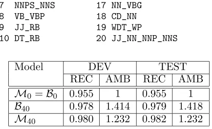
The results of the successive models have been plotted in figure 1 and summarized in table 1, which also shows the results on the test corpus. For each iterationi, recall and ambiguity rates of modelsMiandBion the development corpus were computed. The results show, as expected, that recall and ambiguity rate increase with the increase of the number of ambiguous tags added to the tagset. This is true for both modelsMi andBi. The figure also shows that recall ofBi, for a given i, is generally a bit lower than Mi while its ambiguity is higher. Figure 2 shows that for the same recallBi introduces more am-biguous tags thanMi.
The list of the 20 first ambiguous tags created during the process is represented below :
1 IN_RB 11 IN_WDT_WP 2 DT_IN_WDT_WP 12 VBD_VBN
3 JJ_VBN 13 JJ_NN_NNP_NNS_RB_VBG 4 NN_VB 14 JJ_NN_NNP
5 JJ_NN 15 JJ_NN_NNP_NNS_RB 6 IN_RB_RP 16 JJR_RBR
4
0.95 0.96 0.97 0.98 0.99 1
0 5 10 15 20 25 30 35 40 45 50 1 1.05 1.1 1.15 1.2 1.25 1.3 1.35 1.4 1.45 1.5
recall
ambiguity
iterations recall
ambiguity recall (baseline) ambiguity (baseline)
Figure 1: Recall and ambiguity rate of the suc-cessive models on development corpus
1 1.05 1.1 1.15 1.2 1.25 1.3 1.35
0.955 0.96 0.965 0.97 0.975
ambiguity
recall Model Mi
Baseline
Figure 2: Comparing ambiguity rates for a fixed value of recall
7 NNPS_NNS 17 NN_VBG 8 VB_VBP 18 CD_NN 9 JJ_RB 19 WDT_WP
10 DT_RB 20 JJ_NN_NNP_NNS
Model DEV TEST
REC AMB REC AMB
M0 =B0 0.955 1 0.955 1 B40 0.978 1.414 0.979 1.418 M40 0.980 1.232 0.982 1.232
Table 1: Results on development and test cor-pus
3.1.4 Model efficiency
The original idea of our method consists in cor-recting errors that were made byM0, through the introduction of ambiguous tags. Ideally, we would like models Mi with i > 0 to introduce an ambiguous tag only where M0 made a mis-take. Unfortunately, it is not always the case. We have classified the use of ambiguous tags into four situations function of their influence
on both recall and ambiguity rate as indicated in table 2, whereGstands for the gold standard. In situations 1 and 2 model M0 made a mis-take. In situation 1, the mistake was corrected by the introduction of the ambiguous tag while in situation 2 it was not. In situations 3 and 4, modelM0 did not make a mistake. In situation 3 the introduction of the ambiguous tag did not create a mistake while it did in situation 4.
Situation G M0 Mi REC AMB
1 T1 T2 T1,2 + +
2 T3 T4 T1,2 0 +
3 T1 T1 T1,2 0 +
4 T3 T3 T1,2 − +
Table 2: Influence of the introduction of an am-biguous tag on recall and ambiguity rates
The frequency of each situation for some of the 20 first ambiguous tags has been reported in table 3. The last column of the table indicates the frequency of the ambiguous tag (number of occurrences of this tag divided by the sum of occurrences of all ambiguous tags). The figures show that ambiguous tags are not very efficient: only a moderate proportion of their occurrences (24% on average) actually corrected an error. While we are very rarely confronted with sit-uation 4 which decreases recall and increases ambiguity (0.5% on average), in the vast ma-jority of cases ambiguous tags simply increase the ambiguity without correcting any mistakes. Ambiguous tags behave quite differently with respect to the four situations described above. In the best cases (tag 6), 46% of the occurrences corrected an error, and the tag is used one out of ten times the tagger selects an ambiguous tag, as opposed to tag 19 , which corrected errors in 48% of the cases but is not frequently used. The worst configuration is tag 9, which, although not chosen very often, corrects an error in 13% of the occurrences and increases the ambiguity in 85% of its occurrences.
A more detailed evaluation of the basic tag-ging mistakes has suggested a better adapted and more subtle method of using the ambiguous tags which may at the same time constitute a di-rection for future work. While the vast majority of mistakes are due to mixing up word classes, such as the -ing forms used as adjectives, as nouns or as verbs, about one third of the mis-takes concern only 25 common words such as
ambigu-Tag 1 2 3 4 freq 1 0.220 0.026 0.746 0.006 0.126 5 0.129 0.014 0.852 0.002 0.165 6 0.461 0.000 0.538 0.000 0.107 9 0.133 0.012 0.850 0.003 0.082 19 0.483 0.064 0.419 0.032 0.012 AVG 0.241 0.029 0.722 0.005
Table 3: Error analysis of some ambiguous tags
ous tags for these words alone has yielded a re-call of 0.965 on the test corpus (25% errors less than model M0) while keeping the ambiguity rate very low (1.04). With this procedure, 35% of the ambiguous tags occurrences corrected an error made byM0 and 59% increased the ambi-guity. The result can be improved by designing two sets of ambiguous tags: one to be used for this set of words, and one for the word-classes most often mistaken.
4 Conclusions and Future Work
We have presented a method for computing the probability distributions associated to ambigu-ous tags, denoting subsets of the tagset, in an HMM based part of speech tagger. An iterative method for discovering ambiguous tags, based on the mistakes made by the tagger allowed to reach a recall of 0.982 for an ambiguity rate of 1.232. These figures can be compared to the baseline model which achieves a recall of 0.979 and an ambiguity rate of 1.418 using the same ambiguous tags. An analysis of ambiguous tags showed that they do not always behave in the way expected; some of them introduce a lot of ambiguity without correcting many mistakes.
This work will be developed in two directions. The first one concerns the study of the differ-ent behaviour of ambiguous tags which could be influenced by computing differently the ficti-tious counts of each ambiguous tag, based on its behaviour on a development corpus in order to force or prevent its introduction during tagging. The second direction concerns experiments on supertagging (Bangalore and Joshi, 1999) fol-lowed by a parsing stage the tagging stage asso-ciates to each word a supertag. The supertags are then combined by the parser to yield a parse of the sentence. Errors of the supertagger (al-most one out of 5 words is attributed the wrong supertag) often impede the parsing stage. The idea is therefore to allow some ambiguity during the supertagging stage, leaving to the parser the
task of selecting the right supertag using syntac-tic constraints that are not available to the tag-ger. Such experiments will constitute one way of testing the viability of our approach.
References
Srinivas Bangalore and Aravind K. Joshi. 1999. Supertagging: An approach to almost pars-ing. Computational Linguistics, 25(2):237– 265.
Thorsten Brants. 1995. Tagset reduction with-out information loss. InACL’95, Cambridge, USA.
Thorsten Brants. 2000. Tnt - a statistical part-of-speech tagger. InSixth Applied Natu-ral Language Processing Conference, Seattle, USA.
L. Breiman, J. H. Friedman, R. A. Olshen, and C. J. Stone. 1984. Classification and Re-gression Trees. Wadsworth & Brooks, Pacific Grove, California.
Eugene Charniak, Curtis Hendrickson, Neil Ja-cobson, and Mike Perkowitz. 1993. Equa-tions for part-of-speech tagging. In 11th Na-tional Conference on Artificial Intelligence, pages 784–789.
Philip Clarkson and Ronald Rosenfeld. 1997. Statistical language modeling using the cmu-cambridge toolkit. InEurospeech.
Nelson Francis and Henry Kuˇcera. 1982. Fre-quency Analysis of English Usage: Lexicon and Grammar. Houghton Mifflin, Boston. Mitchell Marcus, Beatrice Santorini, and
Mary Ann Marcinkiewicz. 1993. Building a large annotated corpus of english: The penn treebank. Computational Linguistics, 9(2):313–330, june. Special Issue on Using Large Corpora.
Alexis Nasr and Alexandra Volanschi. 2004. Couplage d’un ´etiqueteur morpho-syntaxique et d’un analyseur partiel repr´esent´es sous la forme d’automates finis pond´er´es. In
TALN’2004, pages 329–338, Fez, Morocco. H. Ney, U. Essen, and R. Kneser. 1994.
On structuring probabilistic dependencies in stochastic language modelling. Computer Speech and Language, 8:1–38.