An Investigation of Radiative Heat Transfer in Fibrous Thin Sheets

ABSTRACT

QASHOU, IMAD. An Investigation of The Radiative Heat Transfer Through Fibrous Thin Sheets. (Under the direction of Dr. Behnam Pourdeyhimi and Dr. Hooman Vahedi

Tafreshi.)

Fibrous materials possess desirable heat transfer characteristics and are used in many thermal applications including thermal insulations. Radiant heat transfer thru such materials is very important even at moderate temperatures. Thus, a fundamental

understanding of the radiative heat transfer through such materials is necessary and allows better evaluation of its insulation capabilities. Due to the complex mathematical

formulation of the theory of radiative heat transfer, the solution of its equations is

consequently as complicated. Computational fluid dynamics (CFD) simulations provide a practical method to understand the response of fibrous media to this electromagnetic irradiation.

diameter. However, SVF has been observed to have the greatest influence followed by the fiber conductivity, and lastly fiber diameter. Fiber thermal conductivity considered in this study are 0.25 - 20 W/m.K and fiber diameters of 20 - 40µm were utilized.

An

Investigation

Of

The

Radiative

Heat

Transfer

Through

Fibrous

Thin

Sheets

by

Imad

Mohammed

Qashou

A dissertation submitted to the graduate faculty of North Carolina State University

in partial fulfillment of the requirements for the degree of

Doctor of Philosophy

Fiber and Polymer Science

Raleigh, NC 2009

APPROVED BY:

___________________________ __________________________

Dr. Peter Hauser Dr. Martin Hubbe

Dedication

Biography

Imad Qashou of Palestinian descent was born on the 8th of January, 1972 in Tripoli, Libya. He completed his Bachelors in Physics from Yarmouk University in Irbid, Jordan. He then joined the physics department at the University of Tennessee, Knoxville where he

Acknowledgements

I would like to thank my committee advisor and friend Dr. Hooman Vahedi Tafreshi, for his support and encouragement through the course of this program. This gratitude is also extended to my other committee advisor Dr. Behnam Pourdeyhimi for providing all the resources required to complete this study and help eliminate all bottlenecks encountered during this time. I would like to thank Dr. Martin Hubbe for agreeing to be my minor committee member. I would like to also acknowledge Dr. Peter Hauser for serving as a member of my advisory committee. Special thanks to Dr. Benoit Maze who has been a great help with the workstations.

Table of Contents

LIST OF TABLES……….……. viii

LIST OF FIGURES……… ix

CHAPTER 1

INTRODUCTION

CHAPTER 2

BACKGROUND

2.1- Nonwovens……….. 5

2.1.1 Definition of Nonwovens………...………….. 5

2.1.1.1 ISO Definition……… 5

2.1.1.2 INDA Definition……… 6

2.1.1.3 ASTM Definition……… 7

2.1.2 Characteristics of Nonwovens……….. 8

2.1.3 Nonwoven Technologies……… 10

2.2- Heat Transfer in Fibrous Media... 15

2.2.1 Conduction……… 15

2.2.2 Convection……… 17

CHAPTER 3

LITERATURE REVIEW

3.1 Radiative Heat Transfer……… 22

3.1.1 The Energy Equation……….. 22

3.1.2 Radiative Transfer Equation……….. 24

3.2 Previous Work on Fibrous Media………. 25

3.2.1 Conduction Model………..……….……….. 28

3.2.2 Radiation Model……….. 30

CHAPTER 4

MODELING RADIATIVE HEAT TRANSFER INSIDE FIBROUS

MEDIA

4.1 S2S and View Factors………..……… 38

4.2 Gray-Diffuse Surfaces and Radiation………..……… 43

CHAPTER 5

NUMERICAL SIMULATION

CHAPTER 6

EXPERIMENTAL

6.1 Materials………..………. 59

6.2 Experimental Specimen………..……….. 59

6.3 Experimental Setup………..………. 60

6.4 Fiber Diameter Measurement………..………. 64

6.5 Basis Weight Measurement………..……… 66

6.6 Thickness Measurement………..………. 67

CHAPTER 7

RESULTS & DISCUSSION

7.1 Mesh Density Study………..……… 73

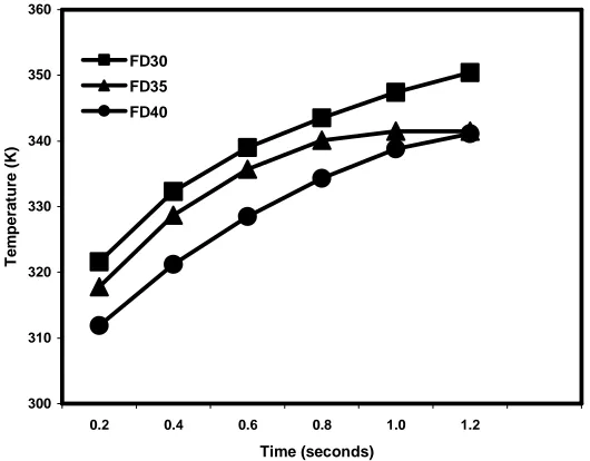
7.2 Fiber Diameter Study………..……….. 74

7.3 Solid Volume Fraction (SVF) Study………..……….. 83

7.4 Thermal Conductivity Study………..……….. 109

7.5 Thickness Study………..………. 119

CHAPTER 8

CONCLUSIONS & RECOMMENDATIONS

REFERENCES

List of Tables

Chapter 3

Table (1) Summary of Conductive Models……… 30

Chapter 6 Table (1) Nonwoven Samples & Characteristics………. 59

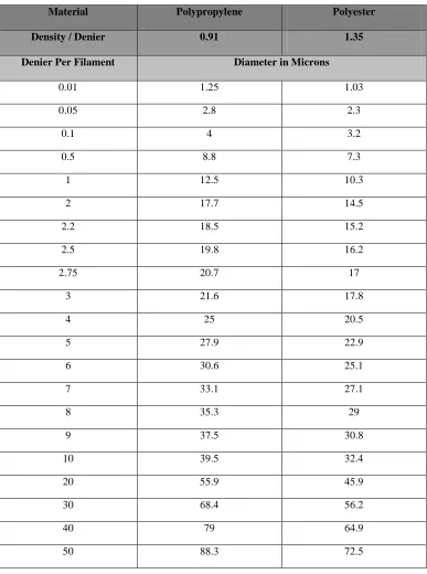
Table (2) Denier vs. Fiber Diameter in Microns……….. 65

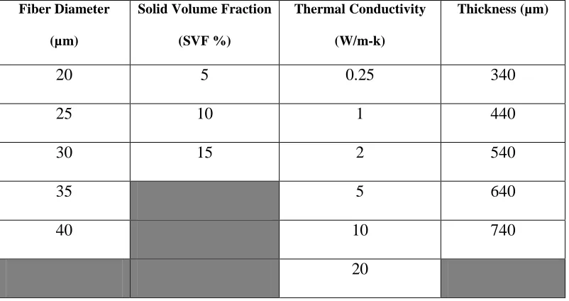
Chapter 7 Table (1) Summary of The Parameters and Variables Considered in This Study……….……… 72

Table (2) Incident Radiation, Fiber Diameter = 20µm……….. 76

Table (3) Incident Radiation, SVF = 5% & Fiber Diameter = 20µm………... 86

Table (4) Incident Radiation, SVF = 10% & Fiber Diameter = 20µm………. 94

Table (5) Incident Radiation, SVF = 15% & Fiber Diameter = 20µm………. 102

Table (6) Incident Radiation, SVF = 5%, Fiber Diameter = 25µm & Conductivity = 0.25 W/m-K……… 111

Table (7) Incident Radiation, SVF = 5%, FD = 30µm, Cond = 0.25 W/m-K & Thickness = 340µm……. 123

Appendix Table (1) View Factors, Thickness Study………. 140

Table (2) View Factors, Conductivity Study……… 141

Table (3) View Factors, Fiber Diameter Study……… 142

Table (4) View Factors, SVF = 5% Study……… 143

Table (5) View Factors, SVF = 10% Study……….. 144

List of Figures

Chapter 2

Figure (1) Example of a Spunbond Web………. 7

Figure (2) Cotton Fibers……….. 8

Figure (3) Wood Pulp Fibers………... 8

Figure (4) Viscose Rayon Fiber………... 8

Figure (5) Shell-Core Fiber Structure……….. 9

Figure (6) Side by Side Bicomponent Fiber Structure……….… 9

Figure (7) Lobal Fibers……… 9

Figure (8) Spunbond Process……….. 11

Figure (9) Spunbond Point-bonded Web……… 11

Figure (10) Carded Thermal Bond Process………. 12

Figure (11) Carded Adhesive Bond Process……… 13

Figure (12) Carded Spunlace Process……….. 13

Figure (13) Ultrasonic Bonding Process………. 14

Chapter 3 Figure (1) Radiative Heat Transfer Process……… 25

Chapter 5 Figure (1) Numerical Simulation Geometry……….………….. 51

Figure (2) Example of Finite Volume Meshes Used in the Study……….. 56

Figure (3) (a-e) Example of the Simulation Temperature Contours Observed in the Study………. 57

Chapter 6 Figure (1) Heat Source Used in the Study………. 60

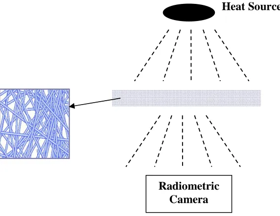
Figure (2) A schematic of the Experimental Setup Used in the Study……….. 61

Figure (3) Infra-red Camera Used in the Study………. 62

Figure (4) A Typical IR Camera Reading……….. 62

Figure (5) Typical IR Camera Experiment Measurements……… 62

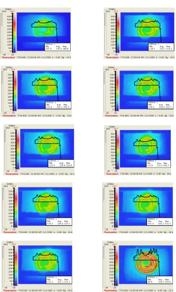
Figure (6) (a-j) Typical Sequence of an IR Experiment………. 64

Figure (7) A Schematic of Denier vs. Fiber Diameter in Microns……… 66

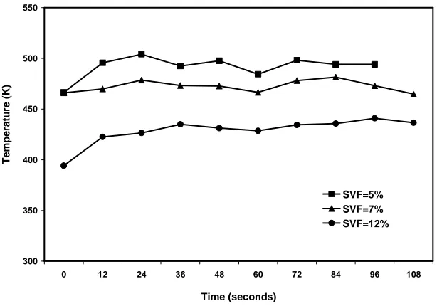
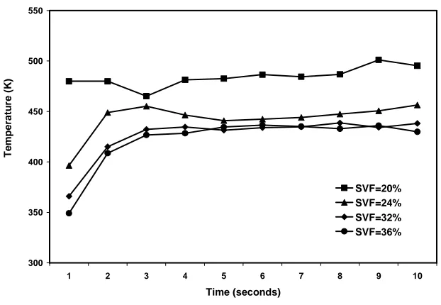
Figure (8) Web Average Temperature for Different Experimental SVF Polyester Webs……… 69

Chapter 7

Figure (1) Mesh Density Study Results………. 73

Figure (2) Average Fiber Temperature Relation with Time for Fiber Diameters = 30, 35 & 40µm @ SVF = 10% , Thickness of 440µm & Thermal Conductivity = 0.25 W/m.K………... 74

Figure (3) Surrounding Fluid Average Temperature Relation with Fiber Diameter………. 75

Figure (4) Temperature Contours of the Fiber Diameter = 20µm @ 0.9 Seconds……….. 77

Figure (5) Temperature Contours of the Fiber Diameter = 25µm @ 0.9 Seconds……….. 77

Figure (6) Temperature Contours of the Fiber Diameter = 30µm @ 0.9 Seconds……….. 78

Figure (7) Temperature Contours of the Fiber Diameter = 35µm @ 0.9 Seconds……….. 78

Figure (8) Temperature Contours of the Fiber Diameter = 40µm @ 0.9 Seconds……….. 79

Figure (9) Incident Radiation vs. Time for Fiber Diameter Study……….. 79

Figure (10) Incident Radiation vs. Fiber Diameter for Fiber Diameter Study……… 80

Figure (11) Incident Radiation vs. Time (Exchange between Heat Source & Fibers)……… 81

Figure (12) Incident Radiation vs. Time (Exchange between Bottom & Fibers)……… 81

Figure (13) Incident Radiation vs. Time (Exchange between Right & Fibers)………... 82

Figure (14) Incident Radiation vs. Time (Exchange between Left & Fibers)………. 82

Figure (15) Incident Radiation vs. Time (Exchange between Fibers & Fibers)………. 83

Figure (16) Average Fiber Temperature vs. Fiber Diameter at Different Solid Volume Fractions………… 84

Figure (17) Average Fiber Temperature vs. Time at Different Solid Volume Fractions……… 85

Figure (18) Surrounding Fluid Temperature Relation with Fiber Diameter at Different Solid Volume Fractions………... 85

Figure (19) Temperature Contours of SVF = 5% & FD = 20µm Simulation………. 87

Figure (20) Temperature Contours of SVF = 5% & FD = 25µm Simulation………. 87

Figure (21) Temperature Contours of SVF = 5% & FD = 30µm Simulation………. 88

Figure (22) Temperature Contours of SVF = 5% & FD = 35µm Simulation………. 88

Figure (23) Temperature Contours of SVF = 5% & FD = 40µm Simulation………. 89

Figure (24) Incident Radiation Monotonic Increase with Time at Different Fiber Diameters for SVF = 5%... 89

Figure (25) Incident Radiation Relation with Fiber Diameters at Different Times for SVF = 5%... 90

Figure (26) Incident Radiation vs. Time (Exchange between Heat Source & Fibers) for SVF = 5%... 90

Figure (27) Incident Radiation vs. Time (Exchange between Bottom & Fibers) for SVF = 5%... 91

Figure (28) Incident Radiation vs. Time (Exchange between Right & Fibers) for SVF = 5%... 91

Figure (29) Incident Radiation vs. Time (Exchange between Left & Fibers) for SVF = 5%... 92

Figure (30) Incident Radiation vs. Time (Exchange between Fibers & Fibers) for SVF = 5%... 92

Figure (31) Surrounding Fluid Temperature vs. Fiber Diameter at Different Times for SVF = 5%... 93

Figure (33) Temperature Contours of SVF = 10% & FD = 25µm Simulation……….. 95

Figure (34) Temperature Contours of SVF = 10% & FD = 30µm Simulation……….. 96

Figure (35) Temperature Contours of SVF = 10% & FD = 35µm Simulation……….. 96

Figure (36) Temperature Contours of SVF = 10% & FD = 40µm Simulation……….. 97

Figure (37) Incident Radiation vs. Time for SVF = 10% at Different Fiber Diameters……… 97

Figure (38) Incident Radiation vs. Fiber Diameter for SVF = 10% at Different Times……… 98

Figure (39) Incident Radiation vs. Fiber Diameter for SVF = 10% (Heat Source-Fibers)………... 98

Figure (40) Incident Radiation vs. Fiber Diameter for SVF = 10% (Bottom-Fibers)………... 99

Figure (41) Incident Radiation vs. Fiber Diameter for SVF = 10% (Right-Fibers)……….. 99

Figure (42) Incident Radiation vs. Fiber Diameter for SVF = 10% (Left-Fibers)………100

Figure (43) Incident Radiation vs. Fiber Diameter for SVF = 10% (Fibers-Fibers)………100

Figure (44) Surrounding Fluid Average Temperature vs. Fiber Diameter for SVF = 10% Study…………101

Figure (45) Temperature Contours of SVF = 15% & FD = 20µm Simulation………..103

Figure (46) Temperature Contours of SVF = 15% & FD = 25µm Simulation………..103

Figure (47) Temperature Contours of SVF = 15% & FD = 30µm Simulation………..104

Figure (48) Temperature Contours of SVF = 15% & FD = 35µm Simulation………..104

Figure (49) Temperature Contours of SVF = 15% & FD = 40µm Simulation………..105

Figure (50) Incident Radiation vs. Time for SVF = 15% at Different Fiber Diameters………105

Figure (51) Incident Radiation vs. Fiber Diameter for SVF = 15% at Different Simulation Times………..106

Figure (52) Incident Radiation vs. Fiber Diameter for SVF = 15% (Heat Source-Fibers)………....106

Figure (53) Incident Radiation vs. Fiber Diameter for SVF = 15% (Bottom-Fibers)………107

Figure (54) Incident Radiation vs. Fiber Diameter for SVF = 15% (Right-Fibers)………...107

Figure (55) Incident Radiation vs. Fiber Diameter for SVF = 15% (Left-Fibers)……….108

Figure (56) Incident Radiation vs. Fiber Diameter for SVF = 15% (Fibers-Fibers)……….108

Figure (57) Surrounding Fluid Average Temperature vs. Fiber Diameter for SVF = 15% Study………….109

Figure (58) Average Fiber Temperature vs. Time for The Thermal Conductivity Study………..110

Figure (59) Temperature Contours of Conductivity = 0.25 W/m-K Simulation @ 0.9 Seconds…………...112

Figure (60) Temperature Contours of Conductivity = 1 W/m-K Simulation @ 0.9 Seconds………112

Figure (61) Temperature Contours of Conductivity = 2 W/m-K Simulation @ 0.9 Seconds………113

Figure (62) Temperature Contours of Conductivity = 5 W/m-K Simulation @ 0.9 Seconds………113

Figure (63) Temperature Contours of Conductivity = 10 W/m-K Simulation @ 0.9 Seconds………..114

Figure (64) Incident Radiation vs. Time at Different Fiber Thermal Conductivities……….114

Figure (65) Incident Radiation vs. Fiber Thermal Conductivities at Different Simulation Times…………115

Figure (66) Incident Radiation vs. Fiber Diameter for Conductivity Study (Heat Source-Fibers)………...115

Figure (67) Incident Radiation vs. Fiber Diameter for Conductivity Study (Bottom-Fibers)………...116

Figure (70) Incident Radiation vs. Fiber Diameter for Conductivity Study (Fibers-Fibers)……….117

Figure (71) Surrounding Fluid Average Temperature vs. Time at Different Fiber Thermal Conductivities………..118

Figure (72) Surrounding Fluid Average Temperature vs. Thermal Conductivity at Different Times……...118

Figure (73) Average Fiber Temperature vs. Thickness for Thickness Study (SVF = 5% & Fiber Diameter = 20µm & Conductivity of 0.25 W/m-K)………120

Figure (74) Average Fiber Temperature vs. Time for the Thickness Study………...120

Figure (75) Experimental Thickness Study………122

Figure (76) Temperature Contours of Thickness = 340µm Simulation @ 0.9 Seconds………124

Figure (77) Temperature Contours of Thickness = 440µm Simulation @ 0.9 Seconds………124

Figure (78) Temperature Contours of Thickness = 540µm Simulation @ 0.9 Seconds………125

Figure (79) Temperature Contours of Thickness = 640µm Simulation @ 0.9 Seconds………125

Figure (80) Temperature Contours of Thickness = 740µm Simulation @ 0.9 Seconds………126

Figure (81) Incident Radiation vs. Time at Different Web Thicknesses………127

Figure (82) Incident Radiation vs. Web Thickness for Different Simulation Times……….127

Figure (83) Incident Radiation vs. Fiber Diameter for Thickness Study (Heat Source-Fibers)……….128

Figure (84) Incident Radiation vs. Fiber Diameter for Thickness Study (Bottom-Fibers)………128

Figure (85) Incident Radiation vs. Fiber Diameter for Thickness Study (Right-Fibers)………...129

Figure (86) Incident Radiation vs. Fiber Diameter for Thickness Study (Left-Fibers)………..129

Figure (87) Incident Radiation vs. Fiber Diameter for Thickness Study (Fibers-Fibers)………..130

Figure (88) Surrounding Fluid Temperature vs. Time at Different Thicknesses………...130

Figure (89) Surrounding Fluid Temperature vs. Thickness at Different Times……….131

CHAPTER 1

Radiative heat transfer through fibrous media has been an area of interest for many years because of the aggressive growth of such media as a thermal insulation from low to elevated temperatures(1). Nonwovens are fibrous materials that are manufactured in different weights and structures, and their widespread use is due to their cost efficient methods of manufacturing. Examples range from the low-cost fiber batting type materials that are typically used in insulations in residential buildings to the more complex and expensive composite materials used in aerospace thermal protection.

The majority of commercial thermal insulations are high-porosity materials that typically contain less than 10% fibers by volume(1). Heat transfers via conduction, convection, and radiation. Most fibrous insulation materials work by lowering the conduction and convection heat transfer, but they are not as efficient in suppressing the radiative heat loss. Radiation is the primary mode of heat transfer through high-porosity fiber thermal insulations even at temperatures above a few hundred Kelvin.

experimental data was generally poor because of inadequate formulation to account for the composition and morphology of the fibrous media (Larkin and Churchill 1959(14); Hottel and Sarofim 1967(15); Tong and Tien 1980(16) and 1983(17); Tong and Yang 1983(18); Houston and Korpela 1982(19); Tong, Swathi and Cunnington 1989(20); Mathes et al. 1990(21); Stark and Fricke 1993(22); and Dombrovsky 1994(23) and 1996(24)).

The objective of the current study is to develop an understanding of the role of fiber diameter, fiber conductivity, and solid volume fraction (SVF) of nonwoven fibrous materials in suppressing the radiative heat transfer. Here, we used the Computational Fluid Dynamics (CFD) code from Fluent Inc. to simulate the temperature and heat flux fields inside 2-D models of nonwoven insulation materials using the Surface-to-Surface (S2S) radiation model. This work is aimed at providing some guidelines for product design and development by studying the effect of the above-mentioned parameters.

CHAPTER 2

2.1 Nonwovens

2.1.1 Definition of Nonwovens:

Since nonwovens are the media of interest in this study, a definition of such media is due and will be beneficial to those who are not practitioners of the technology. There are three main definitions of nonwovens: the ISO, INDA and ASTM definitions.

2.1.1.1 ISO 9092 (now EN 29092)

A manufactured sheet, web or batt of directionally or randomly oriented fibers, bonded by friction, and/or cohesion and/or adhesion, excluding paper and products which are woven, knitted, tufted, stitchbonded incorporating binding yarns or filaments, or felted by wet milling, whether or not additionally needled.

To distinguish wetlaid nonwovens from wetlaid papers, a material shall be regarded as a nonwoven if:

a) more than 50% by mass of its fibrous content is made up of fibers (excluding chemically digested, vegetable fibers) with a length to diameter ratio of greater than 300; of if the conditions in a) do not apply, then,

b) if the following conditions are fulfilled:

i- more than 30% by mass of its fibrous content is made up of fibers (excluding chemically digested vegetable fibers) with a length to diameter ratio greater than 300. And

The commonly used term ‘needlefelt’ has given rise to some confusion since it restrictively associates needling with felting or felt-like products. In fact, needling (mechanical interlocking of fibers by specially designed needles or barbs) is a major method of nonwovens ranging from Medical / hygienic disposables to spunlaid geotextiles.

The appearance of a relatively new group of products such as split-films extruded meshes and nets, etc. presents a further borderline case between nonwoven and related technologies (in this case, plastics).

2.1.1.2 INDA Definition

A sheet, web or batt of natural and/or man-made fibers or filaments, excluding paper, that have not been converted into yarns, and that are bonded to each other by any of several means.

To distinguish nonwovens from papers, a material shall be defined as a nonwoven if: a) more than 50% by mass of its fibrous content is made up of fibers (excluding

chemically digested vegetable fibers) with a length to diameter ratio greater than 300; or

b) more than 30% by mass of its fibrous content is made up of fibers as in a.) above and meeting one or both of the following criteria:

i- length to diameter ratio more than 600 (main quantitative difference between ISO & INDA’s definitions).

Bonding methods may include any of the following means or any combination thereof, including but not limited to:

1. Adding an adhesive

2. Thermally fusing the fibers or filaments to each other or to other meltable fibers or powders.

3. Fusing fibers by first dissolving then re-solidifying their surfaces. 4. Creating physical tangles or tufts among the fibers.

5. Stitching the fibers or filaments in place.

2.1.1.3 American Society for Testing and Materials (ASTM D1117-80)

A textile structure produced by bonding or interlocking, or both, accomplished by mechanical, chemical, or solvent means and combinations thereof.

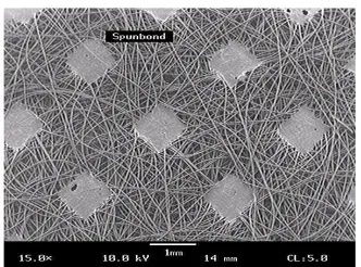
Figure (1) is an example of the spunbond material considered in this study. The fibers are round and randomly distributed thru the web. The size of these fibers can be different depending on the original resins MFR, equipment, process parameters and quench conditions.

2.1.2 Characteristics of Nonwovens

Nonwovens are webs, batts or mats made of filaments or staple fibers which can be natural, manmade or of mineral origin. These filaments or fibers can be deposited at random or can be oriented to various degrees. The filaments or fibers as deposited are then bonded by mechanical, chemical or thermal means.

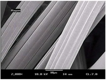
Examples of natural fibers are those made of cotton, wood pulp, viscose Rayon and others like Kenaf and bamboo, etc. Figures (2) – (4) show some of these examples.

Figure (2): Cotton Fibers Figure (3): Wood Pulp Fibers

Figure (4): Viscose Rayon Fibers

be spun into a variety of micro-structures that enhance performance and value of a nonwoven material. Figure (5) – (6) show examples of the different structures. Bicomponent fibers can incorporate a low and high melt components, these fibers are commonly used to bond fibers in different nonwoven technologies including: thermal bond, thru air and hydroentangled bonding. These fibers are also used to bind fibers in thermal insulation webs including fire resistant fabrics.

Bicomponent fiber

Bicomponent fiber

Bicomponent fibers

Bicomponent fibers

Figure (5): Shell – Core Fiber Structure Figure (6): Side by Side Bicomponent Fiber Structure

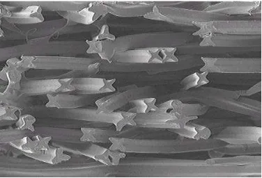
Lobal fibers (tri-lobal, quadralobal, etc.) shown in figure (7) improve the bulk of a web because of the un-orthodox shape of such fibers. Another advantage of such fibers is the improved ability to encapsulate different formulations including: flame retardants and other chemistries based on application and design.

2.1.3 Nonwoven Technologies

For a practitioner of the nonwoven technology, it is fair and representative to say that nonwoven processes can be divided into two categories: spunmelt & carded.

1. Spunmelt

A spunmelt process utilizes thermoplastic resins (pellets, chips, powder form) with a specific Melt Flow Rate (MFR) and viscoelastic properties. Resins used in these technologies include but are not limited to: polyolefins (polypropylene and polyethylene), nylons, polyester and others like PLA. The process starts by melting these resins thru an extruder by use of heat and shear, the molten polymer is pressured thru a spinneret with many tiny holes to form the fibers. The fibers are solidified / crystallized via a quenching process and then laid down on a conveyor belt to be carried into the bonding stage (thru air oven or a calendar) and eventually slit (off or in-line) and wound into roll form.

Spunbond Technology

Melt Extruder SB

Resin

Spinneret

Blow Duct

Cooling Air Heated Calender

Drawing

Conveyor

Winder

Slitter

Surfactant Addition

Figure (8): Spunbond Process

Examples of a point bond spunbond web is shown in Figure (9).

Figure (9): A spunbond Point-bonded Web

2. Carded Nonwovens

is the cause of the different and diverse carded processes, as each is named after the bonding method. These methods include: thermal bonding (a calendar), thru air bonding (hot air thru a rotating cylinder), adhesive bond (via a chemical binder, e.g. latex) and spunlacing or hydroentangling where the bonding of the fibers into a fabric takes place by means of water jets that tie the fibers and filaments into nods resulting in soft and strong webs.

Figures (10) – (12) show schematic of these carded processes:

Thermal Bond Technology

Winder

Fiber Feeding and Opening

Smooth Cylinder Hot Calender Multiple Cards

From

Embossed Cylinder

Chemical Bonding/Gravure Printing

Winder Dry Cans

Gravure Printing Multiple Cards

From Fiber Feeding and Opening

Figure ( 11): Carded Adhesive Bond Process

Spunlacing

Multiple Cards

Winder

From Fiber Feeding and Opening; unwind for roll materials

Multiple H20 Jets

Web Randomizer

Second Entanglement Patterning Section

Chemical Applicator

Dry Cans

Figure (12): Carded Spunlace Process

While the focus of this research is on spunbond webs, the findings of the studies can be extended in a way or another to carded webs and nonwovens in general.

3. Composites

Nonwoven technologies attain further versatility as composites. These are technologies that bond / laminate different layers of nonwovens (similar or different layers) to enhance specific and desired web attributes. The processes could include: calendaring, sonic bonding, hot melt adhesive lamination, etc. Figure (13) shows an example of the ultrasonic laminating process that converts sound into mechanical energy to bond nonwoven materials.

Ultrasonic Laminating & Embossing

Fabric / Film / Paper Unwinds

Ultrasonic Horn

Pattern Roll

Winder

Figure (13): Ultrasonic Bonding Process

reflective with specific emittance and thermal conductive characteristics, thus a customized behavior and interaction with radiative heat transfer and IR waves.

2.2 Heat Transfer in Fibrous Media

Fibrous materials or nonwovens are commonly used as thermal insulations in many engineering systems due to their effective attributes of reducing radiative heat transfer.

Heat transfer though nonwovens occurs by conduction through air and fibers, infrared radiation and also by convection. Radiation heat transfer is found to be the dominant mode of heat transfer at temperatures higher than 400-500K(25). Convention heat transfer is negligible in nonwovens due to the small size of the pores and tortuous nature of air channels.

This research is focused on the most important and dominant heat transfer mode which is the radiative component. However, to understand radiative heat transfer, it is worth providing a brief summary about the nature of heat transfer, the radiative phenomenon and a comparison to the other two heat transfer mechanisms: conduction and convection.

2.2.1 Conduction

more energetic molecules to those with a lower energy level. It can happen is gases, liquids and solids. Higher temperatures are associated with energy and heat is transferred upon the collision of a higher energy molecule with a lower energy one. The empirical law of heat conduction is known as Fourier’s law(26)-(28), which states that the rate of heat flow by conduction is given by:

T k

q=− ∇ (2-1)

The minus sign is a consequence of the fact that heat is transferred in the direction of decreasing temperature.

In the simpler one dimensional form, Fourier’s law can be written as:

A Q dx dT k

q=− = (2-2)

Where, q: the heat flux in the positive x direction, W/m2

Q: rate of heat flow through area A in positive x direction, W. A: area, m2

k: thermal conductivity (the quantity of heat transmitted per unit time per area per unit temperature gradient), W/m-K.

dx dT

2.2.2 Convection

This mode of heat transfer relates to the transfer of heat from a bounding surface to a fluid in motion, or to the heat transfer across the flow plane within the interior of the flowing fluid. If the fluid motion is induced by a pump, a blower, a fan or some similar device, the process is called forced convection. If the fluid motion occurs as a result of the density difference produced by the temperature difference, the process is called free or natural

convection.

When heat takes place between a solid surface and its adjacent fluid, the rate of heat flow can be described by Newton’s law of cooling(26):

q = h (Tw – Tf) = h ∆T (2-3)

where, q : heat flux from the hot wall to the cold fluid, W/m2

∆T: temperature difference between the surface of the wall and fluid mass, K h: heat transfer coefficient, W/m2.K

Tw: temperature of the wall, K

Tf: temperature of the fluid, K

2.2.3 Radiation

and the source of generation. The eye is sensitive to electromagnetic radiation in the area between 0.39 to 0.78µm, which is usually referred to as the visible region of the spectrum. The bulk of thermal radiation takes place in wavelengths ranging from ultraviolet to mid infrared wavelengths including the visible light range and to be more precise from 0.1 to 100µm(28).

J. Stefan’s experimental work and L. Boltzmann’s theoretical work showed that a black surface emits radiant energy at a rate that is proportional to the fourth power of the absolute temperature of the surface. For a black surface, the radiant emission is given by:

Eb = σ A T4 , W or Btu/hr (2-4)

Where, σ is the Stefan Boltzmann constant:

σ = 5.67 x 10-8 W/m2K4 or 1.712 x 10-9 Btu/hr ft2K4

The radiation flux emitted by a real body at an absolute temperature T is always less than that of a black body (perfect absorber and emitter) emissive power Eb and is given by:

q = ε Eb = εσ T4 (2-5)

the black body. However if the radiation is incident on a real body, the energy absorbed, qabs, by the body is given by:

qabs = α qinc (2-6)

where α is the absorptivity and has a value between 0 and 1(28).

Radiative heat transfer is different in many aspects when compared to the other two modes of heat transfer. Radiative heat flux is dependent on the fourth power of temperature, whereas the other two depend on the first power. In addition, radiative heat transfer does not require a medium to transport energy. Thermal radiation, is transferred by electromagnetic waves or photons, which may travel over a long distance without interacting with a medium, this attribute is for great importance in vacuum and space applications.

CHAPTER 3

3.1 Radiative Heat Transfer

Two main equations need to be solved in order to be able to understand and calculate the temperature fields around and inside a fibrous media: the energy equation and the radiative transfer equation (RTE).

3.1.1 The energy equation

The energy equation in its general form is written as follows:

h j

eff j j

eff T hJ S

k p

E v E

t _+

    + − ∇ ∇ = + ∇ + ∂ ∂

_∑

(ρ ρ τ νr

r r

(3-1)

Where keff is the effective conductivity (k + kt where kt is the turbulent thermal

conductivity, defined according to the turbulent model being used), and Jj

r

is diffusion flux of species j. The first three terms on the right side of the equation represent energy transfer due to conduction, species diffusion and viscous dissipation respectively. Sh includes the

heat of chemical reaction and any other volumetric heat sources that have been defined. It also includes radiative source terms if a radiation heat transfer model is used.

E = h -

ρ p + 2 2 v (3-2)

h =

∑

and for incompressible flows:

h = ρ p Y h j j j +

∑

Yj is the mass fraction of species j and:

∫

j c_p,_j dT (3-5)

Tref is 298.15K.

In solid regions, the following form of energy transport equation is used:

[ ]

h v h

t +∇ =∇ ∇ +

∂ ∂ . ) .( )

(

ρ

ρ

where ρ = density

h = sensible enthalpy =

∫

T

Tref cp dT

T = temperature

Sh = volumetric heat source

In this research, Diffusion flux by species is not considered and the main focus is on a distribution of fibers surrounded by an incompressible ideal gas fluid (air in this case). Consequently, viscous and turbulent effects were not of importance to the goals of this study.

3.1.2 Radiative Transfer Equation

In its semi-quasi form, the radiative transfer equation (RTE) is an integro-differential equation that describes the relationships that govern the behavior of radiative heat transfer in the presence of an absorbing, emitting and / or scattering media(30):

' ) ' . ( ) ' , ( 4 ) , ( ) ( ) , ( 4 0 4

2 _{+ Φ Ω}

= +

+ a I r s an T

_∫

σ (3-7)

Where rris a position vector, sris a direction vector, sr'is scattering direction vector, s is path length, a is absorption coefficient, n is the refractive index, σs is the scattering

coefficient, σ is the Stefan-Boltzmann constant (5.672 x 10-8 W/m2-K4), I is the radiation

intensity which depends on position (rr) and direction (sr), T is the local temperature, Φis a phase function and Ω'is the solid angle. (a + σs)s is the optical thickness or opacity of

semi-Figure (1) illustrates the process of radiative heat transfer. Depending on the media under consideration, the incident radiation can be absorbed or scattered by media particles or it can be transmitted thru the media. In addition, the media constituents can emit radiation.

Figure (1): Radiative Heat Transfer Process

To be able to solve the integro-differential RTE equation, traditionally several simplifications and assumptions have been taken into consideration.

3.2 Previous Work on Fibrous Media

consequently the morphology of a web or material was ignored deeming these models limited to a single simplified case and not practical for reasonable simulation or prediction of radiative heat transfer thru such media.

The wide-spread use of light weight fibrous insulation materials in many applications (HVAC, buildings, aircraft, etc.) prompted many studies considering their heat transfer attributes.

Building applications include insulation of walls and attics, such applications will witness rapid growth in the next years due to the awareness of green building and the newly established measures and standards for energy saving. A major drive behind the several studies was the possibilities of reducing cost or material amount without sacrificing insulation value or R-value, specially in a high sales volume industry like that of the construction markets.

shows the importance of radiation and conduction as the main two modes of heat transfer in fibrous media.

In order to reduce heat transfer across a fibrous insulation, gas conduction and/or thermal radiation need to be reduced. Although many concepts for reducing gas conduction were proposed in the past, they are impractical to implement. Examples include: lowering gas pressure requires a vacuum tight system(2,9), the replacement of air by other heavier gases requires a leak proof structure(2,9) and the elimination of intermolecular collisions by creating small cells in the insulation(32). Thus, it is more attractive and practical to control thermal radiation rather than gas conduction.

Many of the past investigations modeled radiative heat transfer in fibrous materials as a conductive process(2,4,6,7,9,11) and developed formula for the thermal conductivity due to radiation. While, these expressions were simple, most of them included a parameter that needed to be determined experimentally. Few studies(14,33) approached the problem from a radiative heat transfer aspect, however their results were not very conclusive.

The following sections will discuss the two models or approaches used by different researchers studying the radiative heat transfer in fibrous media:

3.2.1 Conduction Model

Several researchers(2,4,6,7,9) modeled thermal radiation in fibrous insulations as a conductive process and calculated radiant heat flux q as:

L T k

q= rad ∆ (3-8)

Where krad is the thermal conductivity due to thermal radiation, ∆T is the absolute

temperature difference across the fibrous insulation and L is the thickness of the insulation.

Verschoor and Greebler(2) and Bankvall(9) assumed that thermal radiation propagated through layers of fibers and considered each layer as an absorbing and emitting surface. The net thermal radiation across the entire insulation was found by combining all the contributions among all layers. Strong et al(6), Davies and Birkebak(11) considered the probability of a photon traveling through a differential volume of fibers and derived the radiative thermal conductivity from a different aspect. All researchers mentioned above found that the conductivity due to radiation as:

3 m v

rad T

f r

Where r is the radius of fibers, fv is the volume fraction of fibers and Tm is the mean

temperature in the insulation. The issue with such approach was that different assumptions related to the geometric structure of the fibrous media resulted in different proportionality factors. Furthermore, these factors contained a parameter that describes the extinction of thermal radiation and has to be determined experimentally.

Hager and Steere(7) used a similar approach and obtained a similar krad expression. They

assumed the fibers formed opaque black sheets, thus there was no parameter that needed to be determined experimentally. This approximation was very restrictive, the fiber diameter has to be much larger than the characteristic wavelength of radiation. Therefore, Hager and Steere’s model is strictly valid only for insulations with large fibers (~ 100µm).

Van der Held(4) studied the integral equation governing the radiation passing through fibrous materials. He assumed the temperature gradient in the medium was small and expanded the temperature difference around a point in a Taylor series. Combining the Taylor series and the integral equation, he defined a coefficient associated with the first derivative of the temperature difference as krad. Again, his model contained a factor which

has to be determined experimentally.

Table (1) summarizes the functional dependence of krad derived by the different

size distribution of the fibers. Thus, experiments must be repeated each time any of the three properties is changed.

Table (1): Summary of the Various Conduction Models

Investigator Krad Experimentally Determined

Parameter

Verschoor and Greebler(2)

v m f rT3 2 2 α πσ 2 1

α , opacity factor

Bankvall(9) v m f rT3 2 2 α πσ 2 1

α , opacity factor

Van der Held(4) ₃

3 16 m T ε σ

σ σε , extinction coefficient

Hager and Steere(7)

v m

f

rT3

9σ

None, because assumption that

fibers formed opaque black

sheets

Strong, et al.(6)

v m f T H 3 ∑

πσ ∑ , emissivity

Davis and Birkebak(11)

v m f T F 3 4 ∑

σ ∑ , emissivity

3.2.2 Radiation Model

(product of the back-scattered fraction factor and the scattering coefficient) coefficients. They concluded that the back-scattering coefficients are orders of magnitude larger than the absorption coefficients. This was in agreement with findings cited by Tien and Cunnington(25), who also stated that radiative heat transfer is the major mode of heat transfer in high-porosity insulations at temperatures of excess of 400 – 500 K. They went a further step and tried to predict the coefficients analytically using electromagnetic theory, but due to the unavailability of the complex refractive index for the fibers and computer limitations at that time, only qualitative agreement with experimental values were attained.

Aronson et al.(33) developed expressions for the absorption and scattering coefficients by considering coarse and fine fibers separately. They used the geometrical optics theory and the Rayleigh approximation to estimate the coefficients in the coarse and fine fibers respectively and a bridging formula for those in between. The IR emittance of polypropylene fabrics was calculated with the analytically determined coefficients and compared fairly well with experimental results; however no transfer model was considered in this work.

a- The temperature of the fibers: radiative heat transfer varies directly with the fourth power of absolute temperature.

b- Fiber size: radiation is suppressed by fibers with smaller diameter

c- Fiber volume fraction: there is less heat transfer by radiation through dense fiber assemblies.

d- Emissivity of fibers and bounding surfaces: presence of reflective surfaces reduces radiative heat transfer.

Lee and Cunnington(1) modeled the radiative conductivity of an optically thick medium by a diffusion approximation in which the spectral extinction properties were calculated by a rigorous treatment of the fiber medium scattering phase function and the composition of the fiber material. They modified the classic diffusion model used for optically thick, non-scattering media, to account for the effect of non-scattering by fibers and absorption by the matrix medium (air in this case). The effective total thermal conductivity was given by:

T qL

keff

∆

= (3-10)

Where, q is the total heat flux

L is the thickness of the specimen

According to Lee and Cunnington(1), in the limit of large optical thickness, the keff equation

can be written as:

keff = kr + kc (3-11)

indicating that heat transfer by radiation and conduction are additive for optically thick fibrous insulations.

Xu, et. al.(35). Analyzed the energy absorbing and the temperature variation of the textile upon exposure to infrared. Two equations were established for expressing the temperature increasing and decreasing regulation before and after the infrared was stopped. A useful index β was developed for appraising the textile’s ability of absorbing the infrared energy. The test results showed that the textiles of different materials had different capabilities of infrared absorbing and the textiles coated with ceramic powder, such as ZrC, showed much higher infrared absorbing ability. The temperature decreasing rate had close relation with the textile thickness and temperature increasing rate was related both with infrared absorbing properties and the heat retaining properties. The study further showed that the textiles absorbed energy was usually between 10 – 20% and most of the infrared energy was reflected and transmitted.

Ix = I0 exp (-µx) (3-12)

Where Ix is the infrared intensity at the inner position with the distance of X from the

textile front surface and µ is the infrared absorbing coefficient of the textile. The Lambert-Beer’s law was used by Xu to derive equations for the temperature increasing rate Kx and a

temperature decreasing rate Kr.

ν

C G

h T T

K_{r f a}

⋅ − −

= ( _(max) ) (3-13)

ρ µ

ν ⋅ =

C

K_s (3-14)

Where;

Tf(max) is the textile average temperature at the beginning when the irradiation is stopped. Ta is the temperature of the air surrounding the textile.

h is the heat radiation coefficient of the textile (W/m2.ºC)

G is the weight of the textile unit area (g/m2)

Cν is the textile specific heat capacity (J/g.ºC) µ is the infrared absorbing coefficient of the textile

The experimental setup consisted of an infrared irradiation source and an IR intensity tester. Different samples were exposed to the IR source for 120 seconds and then IR was stopped and the samples were kept for 120 seconds to further test their temperature change.

Tong & Tien(16) concluded that “the study of thermal radiation in light-weight fibrous

insulations is of fundamental importance since a significant portion of the total heat transfer is composed of thermal radiation.” A spectral two-flux model and a method of analytical determination of the radiative properties were developed.

Tong, et. al.(18). conducted two experiments to study radiative heat transfer in light-weight fibrous insulations (LWFI). The spectral extinction coefficients for a commercial LWFI was measured via transmission measurements, and a guarded hot plate apparatus was used to measure the radiant heat flux as well as the total heat flux in the insulation. The experimental results were compared with the theoretical values calculated according to the analytical models reported by the same authors(17,18) in a part I of this part II study. The comparisons revealed that the analytical models were useful in giving representative values for the radiative properties of typical LWFI. However, only qualitative agreements were obtained for the heat transfer results.

calculated at wavelengths from 1.5 to 10.0 µm for several thicknesses of three types of thermal insulating materials having randomly oriented silica fibers of different size distributions. Theoretical results were compared with experimental measurements made on each of the three materials. The theoretical methodology, analytical results, and experimental characterization of geometric parameters and radiative properties of the test materials were presented.

Mohammadi and Banks-Lee(37) presented a theoretical equation of the combined thermal conductive, convective and radiative heat flow through heterogeneous multilayer fibrous materials. Samples whose properties are analyzed by this equation were constructed from glass and ceramic webs and used in an earlier work to experimentally determine their thermal conductivities. In the experimental work, overall effective thermal conductivities were determined using a guarded hot plate instrument with temperatures ranging from 430 to 480˚C. In the theoretical equation presented in the study, thermal convective heat flow is ignored because of the fabric structural conditions, and the conduction component of the overall conductivity is determined by Fricke’s equation(38). Furthermore, the results of the Fricke’s equation and the overall effective thermal conductivity were used to estimate the radiative thermal conductivity of the samples.

CHAPTER 4

4.1 S2S and View Factors

In its semi-quasi form, the radiative transfer equation (RTE) is an integro-differential equation that describes the relationships that govern the behavior of radiative heat transfer in the presence of an absorbing, emitting and / or scattering media:

' ) ' . ( ) ' , ( 4 ) , ( ) ( ) , ( 4 0 4

2 _{+ Φ Ω}

= +

+ a I r s an T

_∫

Where rris a position vector, sris a direction vector, sr'is scattering direction vector, s is path length, a is absorption coefficient, n is the refractive index, σs is the scattering coefficient, σis the Stefan-Boltzmann constant (5.672 x 10-8W/m2-K4), I is the radiation intensity which depends on position ( rr) and direction (sr), T is the local temperature, Φis a phase function and Ω'is the solid angle.

In this chapter the theory behind the Surface-to-Surface model - used in this study - will be discussed. Further the theory behind gray-diffuse surfaces and S2S incorporation of view factors will be also covered.

amount of incident energy upon a surface from another surface is a direct function of the surface-to-surface “view factor,” Fjk.

The view factor Fjk is the fraction of energy leaving surface k that is incident on surface j.

The incident energy flux q_in,k can be expressed in terms of the energy flux leaving all other surfaces as:

jk j out N

j j k

in

kq Aq F

A _,

1

,

∑

=

= (4-2)

Where A is the area of surface k and _k F_jk is the view factor between surface k and surface j. N is the number of surfaces.

The main assumption of the S2S model is that any absorption, emission, or scattering of radiation by the medium can be ignored; therefore, only “surface-to-surface” radiation is considered for analysis. In other words, the exchange of radiative energy between surfaces is virtually unaffected by the medium that separates them.

The energy flux leaving a given surface is composed of directly emitted and reflected energy. The reflected energy flux is dependent on the incident energy flux from the surroundings, which then can be expressed in terms of the energy flux leaving all other surfaces. The following equation was used for the energy reflected from surface k:

k in k k

k

out T q

q _, =ε σ 4+ρ _, (4-3)

Where q_out,k is the energy flux leaving the surface, ε_k is the emissivity, σis the Boltzmann’s constant and q_in,k is the energy flux incident on the surface from the surroundings.

In another form of the aforementioned equation, the radiosity J can be utilized. The total energy given off a surface k is given by:

j N

j kj k

k E F J

J

∑

=

+ =

1

ρ (4-3)

Where Ek represents the emissive power of surface k.

clusters. These values are then distributed to the faces in the clusters to calculate the wall temperatures. The surface cluster temperature is obtained by area averaging as shown in the following equation:

4 / 1 4             =

∑

∑

T (4-4)

Where Tsc is the temperature of the surface cluster and Af and Tf are the area and

temperature of face f. The summation is carried over all faces of a surface cluster.

A smoothing technique is also conducted to enforce the reciprocity relationship and conservation of the view factor matrix. The reciprocity relationship is represented by:

ji j ij

iF A F

A = (4-5)

Where Ai is the area of surface i, Fij is the view factor between surface i and j, and Fji is the

view factor between surfaces j and i. Once the reciprocity relationship has been enforced, a least-squares smoothing method can be used to ensure that conservation is satisfied, i.e.

. 0 . 1

=

These equations along with the energy conservation equation will be solved in this thesis in order to understand the behavior of radiative heat transfer in nonwoven or fibrous webs and more specifically the temperature and heat flux fields will be monitored at different fiber diameter and SVF constructions. Also, the fiber conductivity and web thickness influence on radiative heat transfer will be studied.

For N surfaces, using the view factor reciprocity relationship gives:

Aj Fjk = Ak Fkj for j=1, 2, 3, …, N (4-7)

So that

qin,k =

∑

= N j 1

Fkj qout,j (4-8)

The view factor between two finite surfaces i and j is given by:

Fij =

∫

∫

i

j i i

i

A r

A

A 2

cos cos 1

π θ θ

δij dAi dAj (4-9)

Where δij is determined by the visibility of dAj to dAj. δij is equal to 1 if dAj is visible to

for example the view factor between two infinitely long parallel cylinders of the same diameter 2r and at a distant s apart:

X = 1 +

r s

2 (4-10)

F1-2 = π

1

(sin-1

X

1

+ X2 −1 - X) (4-11)

The emissivity and absorptivity of a gray surface are independent of the wavelength. Also, by Kirchoff’s law(28), the emissivity equals the absorptivity (ε =α). For a diffuse surface, the reflectivity is independent of the outgoing or incoming directions. In this work, the gray-diffuse model is used and the model assumes that if a certain amount of radiant energy (E) is incident on a surface, a fraction (ρ E) is reflected, a fraction (αE) is absorbed, and a fraction (τE) is transmitted. Fluent, the computation fluid dynamics (CFD) code used in this investigation, also assumes that since for most applications the surfaces in question are opaque to thermal radiation (in the infrared spectrum), the surfaces can be considered opaque. The transmissivity, therefore, can be neglected. It follows, from conservation of energy, that α+ρ =1 since ε =α and ρ =1−ε.

4.2 Gray-diffuse Surfaces & Radiation

leaving a surface at location r is composed of two components: emission or emissive power Eb (the subscript b refers to black body) and reflection ρH, where H is the

irradiation of the surface. Consequently the surface radiosity J(r), i.e. the total radiative energy leaving a surface element into the hemisphere, is given by:

J(r) = ε (r) Eb(r) + ρ(r) H(r) (4-12)

Since both emission and reflection are diffuse, so is the resulting intensity leaving the surface:

I(r, ŝ) = I(r) = J(r) /π (4-13)

This means that emitted and reflected radiation can only be distinguished by their different spectral behavior (different wavelengths) and not directional behavior. A gray surface, by definition behaves in the same manner toward all incoming radiation at any wavelengths; consequently a gray surface can not differentiate if its irradiation originates from a gray, diffuse or from a black surface. This simplifies the mathematics significantly as it will allow us to calculate the radiative heat transfer rate and exchange between surfaces by virtue of a balance of the net outgoing radiation (i.e. emission and reflection) traveling directly from surface to surface.

q =qout – qin =(qemission + qreflection) – qirradiation = (E + ρH) – H (4-14)

Using equations (4-12 & 4-14), one can write:

q(r) = ε (r) Eb(r) – α(r) H(r) = J(r) – H(r) (4-15)

The irradiation H(r) is found by determining the contribution from a differential area dA’(r’), followed by integrating over the entire surface. From the definition of the view factor the heat transfer rate leaving dA’ intercepted by dA is (J(r′) dA′) dFdA′ - dA. Thus,

H(r) dA =

∫

J(r′) dFdA′- dA dA′ + H0(r)dA (4-16)

where H0(r) is any external radiation arriving at dA. Using the view factor reciprocity rule

given by equation (4-5), this equation reduces to:

H(r) =

∫

J(r′) dFdA′-dA + H0(r) (4-17)

Substitution into equation (4-15):

q(r) = ε (r) Eb(r) – α(r) [

∫

A

We are now able to calculate the unknown heat flux or temperature if the radiosity field is previously known. Radiosiy field is readily established by solving equation (4-15) for J:

J(r) = ε (r) Eb(r) + ρ (r) [

∫

A

J(r′) dFdA′ - dA + H0(r)] (4-19)

For those surface locations with known temperatures or for those parts of the surface where the local heat flux is given:

J(r) = q(r) +

∫

J(r′) dFdA - dA′+ H0(r) (4-20)

If we now invoke the assumption of gray, diffuse surfaces, or α = ε :

q(r) = ) ( -1

) (

r r

ε ε

[Eb(r) – J(r)] (4-21)

Solving for radiosity:

J(r) = Eb(r) – ( 1

) ( 1 ₋

r

ε ) q(r) (4-22)

) ( ) ( r r ε q -

∫

ε ) q(r′) dFdA - dA′ + H0(r) = Eb(r) -

∫

A

Eb(r′) ) dFdA - dA′ (4-23)

It is customary to break up a gray enclosure into N subsurfaces, over each of which the radiosity is assumed constant(29). Then equation (4-19) becomes

) ( ) ( i i i i q r r

ε = Ebi(ri) -

∑

= N j 1

Jj Fi-j - H0i(ri) i=1,2,…, N (4-24)

Averaging over subsurface Ai :

i i

q

ε = Ebi -

∑

= N j 1

Jj Fi-j - H0i i=1,2,…, N (4-25)

Also, averaging of equation (4-21) gives:

qi =

i i ε ε

-1 [Ebi – Ji] (4-26)

Solving for J and substituting into equation (4-25), we obtain:

i i q ε -

∑

- 1) Fi-j qj + H0i = Ebi -

∑

= N j 1

Using the summation rule of the view factors

∑

= N j 1

Fi-j = 1, we may also re-write equation

(4-27) as an interchange between surfaces,

i i q ε -

∑

- 1) Fi-j qj + H0i =

∑

= N j 1

Fi-j (Ebi - Ebj ) , i = 1, 2, …, N (4-28)

Equation (4-27) is preferred for open configurations, since it allows one to ignore hypothetical closing surfaces; and equation (4-28) is preferred for closed enclosures, because it eliminates transfer between surfaces at the same temperature.

For specific applications the radiosity of a surface needs to be determined, for example, relating surface temperature to radiative intensity leaving a surface. Depending on which of the two is unknown, elimination of qi or Ebi from equation (4-25) with the help of

equation (4-26) leads to:

Ji = εiE_bi + (1- εi) [

∑

= N j 1

Jj Fi-j + H0i ] = qi +

∑

= N j 1

Jj Fi-j + H0i , i = 1, 2, …, N (4-29)

The Kronecker delta is usually introduced into equation (4-27) for the purposes of computer calculations, thus:

∑

- ( ε 1

- 1) Fi-j ] qj =

∑

N

If all the temperatures are known and the radiative heat fluxes are to be determined, equation (4-27) may be cast in matrix form as:

C . q = A . eb – h0 (4-31)

Where C and A are matrices with elements:

Cij =

j ij ε δ

- ( i ε 1

- 1) Fi-j (4-32)

Aij = δij - Fi-j (4-33)

and q, eb and h0 are vectors of the unknown heat fluxes qj and the known emissive powers

Ebj and external irradiation H0j. Equation (4-31) is solved by matrix inversion as:

CHAPTER 5

Nonwoven sheets are 3-D layered structures. Such structures consist of a large number of fibers randomly distributed in a horizontal plane and sequentially deposited on top of each others to build a 3-D layered geometry. Since this study is focused only on the radiative heat transfer through the material’s thickness, we conduct our simulations in 2-D

geometries representing the media’s cross section to reduce the calculation’s CPU time. In our model (Figure (1)), fibers are modeled as circles arranged inside a domain representing the thickness of the fibrous media. Here a simulation domain of 440µm is considered as this is a representative thickness of thin sheet nonwoven materials.

Figure (1): Geometry Used in this Study

Boundary conditions considered in the simulations are as follows: the top and bottom boundaries are considered to be walls with constant temperatures. The walls in the simulation were adiabatic, i.e. heat flux = 0. The top wall will serve as the heat source (at 500K), while the bottom wall and the fibers are heat sinks (300K). Pressure outlet boundary conditions are used on the sides of the simulation domain. The top wall temperature was intentionally chosen to be lower than the fibers (polyester) melting point

TOP

RIGHT LEFT

(around 533K). The emissivity of all boundaries is set to 1. The medium is assumed to be filled with air with an incompressible-ideal-gas density. Solid phase (fibers) is considered to be Polyester with a density of 1540 kg/m3, heat capacity of 2000 j/kg-k and thermal conductivity of 0.25 w/m-k.

Wall boundary conditions in Fluent are used to bound fluid and solid regions. The parameters defined for such boundary condition are both thermal and radiation ones. Thermal boundary conditions include: heat flux, temperature and external radiation heat transfer. A fixed value for temperature was chosen for each wall, the heat flux from a cell is computed as:

rad f

w

f T T q

h

q= ( − )+ (5-1)

Where,

hf = fluid-side local heat transfer coefficient

Tw = wall surface temperature

Tf = local fluid temperature

qrad = radiative heat flux

rad s w s q T T n k

q − +

∆

= ( ) (5-2)

Where,

ks = thermal conductivity of the solid

Ts = local solid temperature

∆n = distance between wall surface and the solid cell center.

The heat flux boundary condition at a wall is defined by specifying the heat flux at the wall surface using the following equation:

f f rad w T h q q

T = − + (5-3)

When the wall borders a solid region, the wall surface temperature is computed as:

s s rad w T k n q q

T =( − )∆ + (5-4)

When external radiation boundary condition is used, the heat flux to the wall is computed as: ) ( ) ( )

( w f rad ext ext w ext 4 w4

f T T q h T T T T

h

Pressure outlet boundary conditions require the specification of a static (gauge) pressure at the outlet boundary. The value of the specified static pressure is used only while the flow is subsonic. Should the flow become locally supersonic, the specified pressure will no longer be used; pressure will be extrapolated from the flow in the interior. All other flow quantities are extrapolated from the interior. Inputs of a pressure outlet include: static pressure, backflow conditions (mainly total stagnation temperature for energy calculations) and radiation parameters. Radiation is defined by specifying the internal emmissivity.

An unsteady state model has been adopted for this study. The finite volume method implemented in Fluent code is used to solve the energy equation. Note that energy equation is the only governing equation to be solved as radiation is believed to be the dominant heat transfer mechanism.