| GENOMIC SELECTION
Genomic Prediction from Multiple-Trait Bayesian
Regression Methods Using Mixture Priors
Hao Cheng,*,1Kadir Kizilkaya,†Jian Zeng,‡Dorian Garrick,§and Rohan Fernando**
*Department of Animal Science, University of California Davis, California 95616,†Department of Animal Science, Adnan Menderes University, Aydin, 9100 Turkey,‡Program in Complex Trait Genomics, Institute for Molecular Bioscience, University of Queensland, St Lucia, QLD 4072, Australia,§School of Agriculture, Massey University, Palmerston North 4442 New Zealand, and **Department of Animal Science, Iowa State University, Ames, Iowa 50011-1050 ORCID IDs: 0000-0001-5146-7231 (H.C.); 0000-0001-8640-5372 (D.G.); 0000-0001-5821-099X (R.F.)
ABSTRACTBayesian multiple-regression methods incorporating different mixture priors for marker effects are used widely in genomic prediction. Improvement in prediction accuracies from using those methods, such as BayesB, BayesC, and BayesCp, have been shown in single-trait analyses with both simulated and real data. These methods have been extended to multi-trait analyses, but only under the restrictive assumption that a locus simultaneously affects all the traits or none of them. This assumption is not biologically meaningful, especially in trait analyses involving many traits. In this paper, we develop and implement a more general multi-trait BayesCPand BayesB methods allowing a broader range of mixture priors. Our methods allow a locus to affect any combination of traits, e.g., in a 5-trait analysis, the“restrictive”model only allows two situations, whereas ours allow all 32 situations. Further, we compare our methods to single-trait methods and the“restrictive”multi-trait formulation using real and simulated data. In the real data analysis, higher prediction accuracies were observed from both our new broad-based multi-trait methods and the“restrictive” formulation. The broad-based and restrictive multi-trait methods showed similar prediction accuracies. In the simulated data analysis, higher prediction accuracies to the“restrictive”method were observed from our general multi-trait methods for intermediate training population size. The software tool JWAS offers open-source routines to perform these analyses.
KEYWORDSmulti-trait; mixture priors; genomic prediction; Bayesian regression; pleiotropy; GenPred; Shared data resources; Genomic Selection
G
ENOMIC prediction was proposed by Meuwissen et al. (2001) to incorporate marker effects from whole-genome data into genetic evaluation. In genomic prediction, all the marker or haplotype effects are estimated simultaneously, and these estimates can then be used to predict breeding val-ues of individuals not in the training population used to esti-mate the effects.Bayesian multiple-regression methods incorporating mix-ture priors for marker effects are used widely in genomic prediction, including various extensions to the BayesB method of Meuwissen et al.(2001). BayesB accommodates models where the prior for each marker effect follows a mixture dis-tribution with a point mass at zero with probabilitypand a
univariate-t distribution with probability 12p (Meuwissen et al.2001; Gianolaet al.2009; Chenget al.2015b). Another model, BayesC, assumes a mixture with a point mass at zero with probabilitypand a univariate normal distribution with probability 12p for all marker effects, and its extension known as BayesCpfurther treatspas an unknown parameter with a uniform prior distribution (Habieret al.2011).
Bayesian multiple-regression methods werefirst proposed for single-trait analyses but have been extended to some particular forms of multi-trait analyses (Calus and Veerkamp 2011; Jia and Jannink 2012). Those extensions have per-tained to a particular, somewhat restrictive mixture model. The “restrictive”multi-trait BayesCP presented by Jia and Jannink (2012) assumes any particular locus affects none of the traits or simultaneously affects all traits. This assump-tion of genetic architecture in that multi-trait BayesCPmodel is violated if some loci have no effect on at least one of the traits while having an effect on the remaining traits.
In this paper, we propose a more general class of multi-trait BayesCPand BayesB methods, where each locus can have an
Copyright © 2018 by the Genetics Society of America doi:https://doi.org/10.1534/genetics.118.300650
Manuscript received December 18, 2017; accepted for publication March 2, 2018; published Early Online March 7, 2018.
Supplemental material is available online atwww.genetics.org/lookup/suppl/doi:10. 1534/genetics.118.300650/-/DC1.
1Corresponding author: 2139 Meyer Hall, Department of Animal Science, University
effect on any combination of traits. For example, in a 5-trait analysis, the restricted model only allows two situations, whereas ours allows all 32 situations. The previous restric-tive multi-trait models are special cases of this general class of models. Further, our model allows the use of a single-site Gibbs sampler that requires less computing effort than some alternative Markov chain Monte Carlo approaches, espe-cially for analyses involving many traits. Methodologies for the new models are compared to single-trait methods and the previous multi-trait methods using real and simu-lated data.
Materials and Methods
Multi-trait marker effects model
For simplicity of our description, but without loss of gener-ality, we will assume individuals have all traits measured with a general mean as the onlyfixed effect, and write the multi-trait model for individualifromngenotyped individ-uals as
yi¼mþX
p
j¼1
mijajþei;
whereyiis a vector of phenotypes ofttraits for individuali,m
is a vector of overall means forttraits,mij is the genotype
covariate at locusjfor individuali(coded as 0,1, and 2),pis the number of genotyped loci,ajis a vector of allele
substi-tution effects or marker effects ofttraits for locusj, andeiis a
vector of random residuals of t traits for individuali. The
fixed effects, or general mean in this case, are assignedflat priors. The residuals,ei;area prioriassumed to be
indepen-dently and identically distributed multivariate normal vec-tors with null mean and covariance matrix R; which, in turn, is assumed to have an inverse Wishart prior distribution, Wt21ðSe;neÞ:
We will show that, employing the concept of data aug-mentation, the vector of marker effects at a particular locus
ajcan be written asaj¼Djbj;whereDjis a diagonal matrix
whosekth diagonal entry is an indicator variable indicating whether the marker effect of locus jfor traitk is zero or nonzero, andbjfollows a multivariate normal distribution
in multi-trait BayesCPor a multivariatetdistribution in multi-trait BayesB.
Multi-trait BayesCPmodel
Priors for marker effects:The prior forajk;the allele
sub-stitution or marker effect of traitkfor locusj, is a mixture with a point mass at zero and a univariate normal distribution conditional ons2k:
ajkjpk;s2k
N0; s2k
probabilityð12pkÞ
0 probability pk
and the covariance between effects for traitskandk9at the same locus,i.e.,ajkandajk9is
covðajk;ajk9jskk9Þ ¼
skk9 if both ajk6¼0 and ajk96¼0
0 otherwise :
The vector of marker effects at a particular locusajis written
as aj¼Djbj; where Dj is a diagonal matrix with elements
diagðDjÞ ¼dj¼ ðdj1;dj2;dj3. . .djtÞ;where djkis an indicator
variable indicating whether the marker effect of locus jfor traitkis zero or nonzero, and the vectorbjfollows a
multi-variate normal distribution with null mean and covariance
matrix G¼ 2 4s
2
1 ⋯ s1t
⋮ ⋱ ⋮
s1t ⋯ s2t
3
5 The covariance matrix Gis a
priori assumed to follow an inverse Wishart distribution, W21
t ðSb;nbÞ:Thus, the multi-trait BayesCPmodel with data augmentation is written as
yi¼mþX
p
j¼1
mijDjbjþei: (1)
In the most general case, any marker effect might be zero for any possible combination of ttraits resulting in 2t possible
combinations ofdj:For example, in at=2 trait model, there
are 2t¼4 combinations ford
j:ð0; 0Þ;ð0; 1Þ;ð1; 0Þ;ð1; 1Þ:
In the restrictive special case of this model described by Jia and Jannink (2012), only two combinations,i.e.,ð0; 0Þand
ð1; 1Þ;have nonzero probability. Suppose, in general, we use numerical labels“1,” “2,”. . .;“l”for the 2tpossible outcomes
fordj;then the prior fordjis a categorical distribution
pðdj¼“i”Þ ¼P1Iðdj¼“1”Þ þP2Iðdj¼“2”Þ þ. . .
þPlIðdj¼“l”Þ;
where Pli¼1Pi¼1 withPi being the prior probability that
the vectordjcorresponds to the vector labeled“i”:A Dirichlet
distribution with all parameters equal to one,i.e., a uniform distribution, can be used for a prior forP¼ ðP1;P2;. . .;PlÞ:
As shown below, we consider two Gibbs samplers to draw samples for all the parameters in this model. Gibbs sampler I is a single-site sampler, where only one of the tindicator labels is sampled at a time. Thus, in a 2-trait model, for ex-ample, this sampler cannot move fromð0; 0Þtoð1; 1Þ in a single step without stepping throughð1; 0Þorð0; 1Þfordj:
Therefore, Gibbs sampler I cannot be used for the restrictive model which excludesð1; 0Þandð0; 1Þfrom the state space fordj:Gibbs sampler II, however, samples all elements ofdj
jointly, and can move fromð0; 0Þtoð1; 1Þin a single step. However, Gibbs sampler II is computationally more intensive because it requires drawing samples from a multivariate nor-mal distribution of ordert, the number of traits.
Gibbs sampler I for multi-trait BayesCP:Suppose the prior fordjis a categorical distribution for which the support is the set
of 2toutcomes of
dj:For convenience, from now on let“1”
de-note trait k and “2” the other t21 traits. In our sampling scheme,bj1anddj1are sampled from their joint full conditional
conditional distribution of bj1 givendj1 and the marginal full
conditional distribution ofdj1:Letudenote all other
param-eters except dj1 andbj1;then our sampling scheme can be
written as
f
bj1;dj1u;y
¼f
bj1dj1;u;y
f
dj1u;y
:
The full conditional distributions ofbj1;dj1;P;GandRfor
Gibbs sampler I, whose derivations are in the Appendix, are given below. The full conditional distributions ofbj1is
p
bj1dj1;u;y
¼ N
b b0j1;
G1121 when dj1¼0
N
b b1j1;
C1
j;11 21
when dj1¼1
; 8 > > > < > > > : with b b0j1¼ 2
G11
21
G12
bj2;
b b1j1¼
C1j;11
21
rj12C1j;12bj2
;
Cj1;11¼G11þR11X n
i¼1 m2ij
C1
j;12¼G12þR12Dj2 Xn
i¼1 m2ij;
rj1¼ Xn
i¼1 w9imij
!" R11 R21 #
;
wherewi¼yi2m2
P
j96¼jmij9Dj9bj9;G11andG12are the par-titions ofG21 corresponding to traitk and covariances be-tween traitkand other traits, respectively.R11andR12
are the partitions of R21 corresponding to traitk and covariances between traitkand other traits, respectively.
The marginal full conditional probability thatdj1¼1 is
fdj1¼1u;y¼
n
1þ Pr
dj1¼0;dj2P
Pr
dj1¼1;dj2P H
!
21o
21;
whereH¼
exp
n
21
2 logC
1 j;112bc1j1
2 Cj1;11
!
2 21
2
logG112bc0j1 2
G11
!
o
:The full conditional distribution forPcan be written as
fPb;D;G;R;y}Dirichletn1þ1; n2þ1;. . .
;
whereniis the number of loci or markers for whichdj¼“i”:
The full conditional distributions for R; the covariance matrix for residuals, is an inverse Wishart distribution, W21
t ðSeþe9e;neþnÞ;whereeis then3tmatrix for
resid-uals whoseith row ise9i:The full conditional distribution for
G;the covariance matrix forbj;is an inverse Wishart
distri-bution, W21
t ðSbþb9b;nbþpÞ;wherebis thep3tmatrix whoseith row isb9i:
Gibbs sampler II for multi-trait BayesCP:The Gibbs sam-pler above, where only one of thetindicator labels is sampled at a time, cannot be used for the restrictive model assuming any particular locus affects all traits or none of them. Further, if some particularPiare near zero, the chain might exhibit
mixing problems. Another, more general, but computation-ally intensive, Gibbs sampler that samples all elements ofdj
jointly and may exhibit improved mixing is proposed below. The full conditional distributions ofbj;dj;P;G;andRfor
Gibbs sampler II, whose derivations are in the Appendix, are given below.
Letudenote all other parameters except bjanddj;then
our sampling scheme can be written as
f
bj;dju;y
¼f
dju;y
f
bjdj;u;y
:
The full conditional distribution ofbjis
f
bjdj;u;y
}N
C2j 1rj;C2j 1
;
whereCj¼D9jR21Dj
Pn
i¼1m2ijþG2
1
and r9j¼
Pn i¼1w9imij
R21Dj:
The marginal full conditional probability ofdj¼“i”is
fðdj¼“i”ju;yÞ
¼ f
ydj¼“i”;u
fdj¼“i”P
P
“i”2f“1”;“2”;...;“l”gf
ydj¼“i”;u
f
dj¼“i”P ;
where
f
ydj;u
¼C21 j 1 2 exp
n
1 2r 9jC2j 1rj
o
:
This Gibbs sampler can accommodate the“restrictive”multi-trait BayesCPthat was proposed by Jia and Jannink (2012), which only allowsdjto be a vector of all ones or a vector of all zeros.
Multi-trait BayesB model
The multi-trait BayesCPmodel proposed above can be mod-ified to accommodate the general multi-trait BayesB model. Model Equation (1) can also be used for the multi-trait BayesB method. The differences in multi-trait BayesB method is that the prior forbjis a multivariatetdistribution, rather
than a multivariate normal distribution. This is equivalent to assumingbjhas a multivariate normal distribution with
null mean and locus-specific covariance matrixGj;which is
assigned an inverse Wishart prior,W21
The derivations of the full conditional distributions of parameters of interest for Gibbs samplers are shown in the Appendix. In the multi-trait BayesB model, the full conditional distributions for all parameters exceptGjare similar to the
multi-trait BayesCPmodel. The full conditional distribution for Gj; the covariance matrix forbj; is an inverse Wishart
distribution,W21
t ðSbþbjb9j;nbþ1Þ:
Data analyses
Real data: Published genotypic and deregressed breeding values based on phenotypic data for Loblolly Pine (Pinus taedaL.) were used (Resendeet al.2012; Daetwyleret al.2013). Two disease traits, namely presence or absence of rust (Rust_bin) and gall volume (Rust_gall_vol) were analyzed. These are the two traits used in Jia and Jannink (2012). The reported heritabilities were 0.21 for Rust_bin and 0.12 for Rust_gall_vol. Loci with missing genotypes were imputed as the mean of the observed genotype covariates at that locus but loci with a missing rate .50% were excluded. After these quality control edits, 4828 SNPs on 807 individuals with deregressed phenotypes and genotypes on both traits remained.
Prediction accuracy was calculated as the correlation be-tween the vector of deregressed phenotypes and the vector of estimated breeding values. Cross-validation using 10 folds formed the basis for comparing these methods. Pairedt-tests were used for tests of significance of difference in prediction accuracies between two methods, where prediction accura-cies for two different methods from each validation fold were considered as paired samples. The general multi-trait BayesCPmodel (MT-BayesCP-G) was compared to a simi-lar model where the prior for aj is a multivariate normal rather than a mixture of multivariate normals (MT-BayesC0), the more restricted multi-trait BayesCP proposed by Jia and Jannink (2012) (MT-BayesCP-R) and the usual single trait formulations of the mixture models (ST-BayesC0, ST-BayesCp). Since BayesC0 is equivalent to random regres-sion best linear unbiased prediction (RR-BLUP), ST-BayesC0 and MT-BayesC0 are denoted as ST-RR-BLUP and MT-RR-BLUP below. The prior for the residual covariance matrix
R in all multi-trait methods was an inverse Wishart
distri-bution, W21¼
0:003 0 0 0:003
;6 ;for which the mean
of R is
0:001 0 0 0:001
;the SD of diagonal elements are
1:431023;and the SD of off-diagonal elements are 0. This
same prior was used for the marker effects covariance ma-trix G:The priors for the residual variance and marker ef-fects variance in single-trait analyses were scaled inverted chi-squared distributions with scale parameterS2¼0:0005
and degrees of freedom n¼4;for which the mean of the prior was also 0.001. In the data analyses, multi-trait BayesB methods provided similar results as multi-trait BayesCP methods. Thus, only results from BayesCPanalyses were presented below to demonstrate the superiority of our multi-trait methods.
Simulated data:Simulated data described below were used to quantify the superiority of the general multi-trait Bayesian methods. Two scenarios were simulated. In scenario 1, as a known ideal condition, the simulated genome consisted of 100 loci on each of two chromosomes that were in Hardy-Weinberg and linkage equilibria. All these loci were consid-ered as QTL or causative variants and used in the analyses. The QTL on thefirst chromosome had effects only on trait 1 and those on the second chromosome only on trait 2. The effects of these QTL were simulated from a standard normal distribution and then were equally scaled to provide unit genetic variance for each trait in the simulated population of 8000 unrelated individuals. The phenotypes for these traits were obtained by adding independent residuals to the genetic values. Two situations were simulated: (1) her-itabilities for both traits were 0.5; (2) heritability for trait 1 was 0.2 and for trait 2 was 0.8. The XSim package was used in the simulation (Supplemental Material, File S1) (Chenget al.2015a).
In scenario 2, both markers and QTL were simulated. The simulated genome consisted of 100 evenly spaced loci on each of three chromosomes of length 10 cM. Ten loci were randomly selected on each chromosome as QTL. Allele states were sampled from a Bernoulli distribution with fre-quency 0.5 in the base population. Starting from a base population of 500 males and 500 females, random mating was simulated for 500 generations to generate linkage dis-equilibrium. Random mating was continued forfive more generations to increase the population size to 4000 males and 4000 females, which were used in the analyses. The effects of QTL on thefirst two chromosomes were simulated following the same strategy in scenario 1,i.e., the QTL on thefirst chromosome had effects only on trait 1, and those on the second chromosome only on trait 2. All QTL on the third chromosome had effects on both traits. The effects of these QTL on the third chromosome were simulated from a standard bivariate normal distribution with correlation 0.5. The phenotypes for these traits were obtained by add-ing independent residuals to the genetic values. In total, 8000 individuals were simulated with heritability 0.2 for trait 1 and 0.8 for trait 2.
The same validation approaches were used for these two simulation scenarios. A total of 500 individuals were used for testing, and for each training population of sizeN, 100 repli-cates of the training population were sampled from the remaining individuals. The values considered for N were 50, 100, 200, 400, 1000, 2000, 4000, or 7000. The true ge-netic and residual variances were used to compute the scale parameters for the priors of the variance components. The general multi-trait BayesCP model (MT-BayesCP-G) was compared to the more restricted multi-trait BayesCP (MT-BayesCP-R) using this dataset.
Data availability
The genotypic and phenotypic data used in the real data analysis are publicly available (Resende et al. 2012). The scripts used to generate the simulated data are provided as supplementary information. The authors state that all data necessary for confirming the conclusions presented in the article are represented fully within the article.
Results
Real data
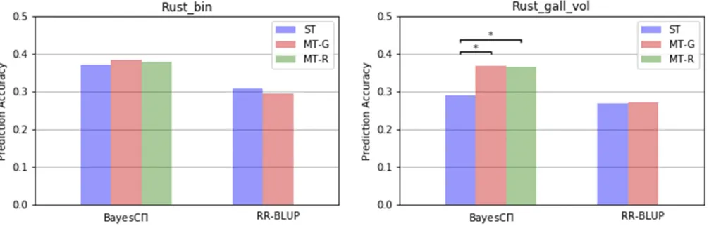
The prediction accuracies from all methods for Rust_bin and Rust_gall_vol are in Figure 1. The prediction accuracies from all single-trait analyses using JWAS are similar to those in Resendeet al.(2012).
The predictions of Rust_bin exhibited no significant differ-ence in accuracy between multi-trait and single-trait analyses within each method (ST-RR-BLUPvs.MT-RR-BLUP; ST-BayesCp vs.MT-BayesCP-R; ST-BayesCpvs.MT-BayesCP-G).
In contrast, prediction accuracies for the lower heritability Rust_gall_vol with MT-BayesCP-G were significantly higher than those from ST-BayesCp. MT-BayesCP-G and MT-BayesCP-R showed similar prediction accuracies. The posterior means ofP for both methods are in Table 1. When RR-BLUP was used for the analysis, however, the advantage of the multiple-trait analysis (MT-RR-BLUP) over the single-trait analysis (ST-RR-BLUP) for Rust_gall_vol was not observed.
Simulated data
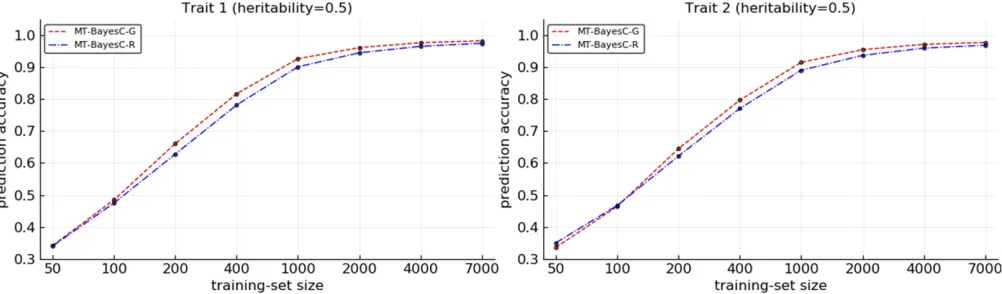
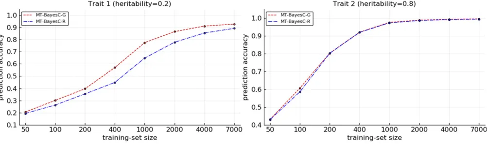
The prediction accuracies from MT-BayesCP-G and MT-BayesCP-R methods were compared for varying size (N) of training populations under two simulation scenarios. In sim-ulation scenario 1, Figure 2 shows the prediction accuracies where heritabilities for both traits were 0.5. Figure 3 shows the prediction accuracies where heritabilities for trait 1 and trait 2 were 0.2 and 0.8, respectively. When N¼50;both methods had similar prediction accuracy. For both traits, as N increased, initially, MT-BayesCP-G became superior to
MT-BayesCP-R, but, as expected, the accuracies of these methods asymptotically converged (Karaman et al. 2016). In most cases, the differences in accuracies for both traits were small. However, in Figure 3, the differences in accura-cies for trait 1, for which the heritability was 0.2, were sub-stantial for intermediate values of N. Figure 4 shows the prediction accuracies for simulation scenario 2. The pattern observed is similar to Figure 3 under simulation scenario 1. MT-BayesCP-G was superior to MT-BayesCP-R for intermedi-ate training population, but asNincreased, the accuracies of these methods asymptotically converged (Karamanet al.2016).
Discussion
Real data
Significant differences between multi-trait and single-trait analyses were only observed for Rust_gall_vol within BayesCp methods (MT-BayesCP-Gvs.ST-BayesCp; MT-BayesCP-R vs. ST-BayesCp). MT-BayesCP-G and MT-BayesCP-R out-performed ST-BayesCpfor Rust_gall_vol, and the accuracy gain was 26% (from 0.287 to 0.364). The lower-heritability trait Rust_gall_vol benefited from information on the other correlated trait Rust_bin. Thus higher prediction accuracy from MT- BayesCP-G were observed in trait Rust_gall_vol but not for the high heritability Rust_bin. Results in Jia and Jannink (2012) showed no difference between MT-BayesCP and ST-BayesCpbecause a reduced marker panel (500 markers) was used.
The fact that RR-BLUP showed no improvement in multi-trait analyses suggested that benefits from MT-BayesCP-G may be due to the estimation of the hyper-parameterP:In the MT-BayesCP-G, the mean of the posterior probability that a marker has a null effect on Rust_gall_vol was0.97, calculated as the summation of posterior mean ofPfor cat-egoriesð0;0Þandð1;0Þ:The posterior mean ofp, the prob-ability that a marker has a null effect, in ST-BayesCp for Rust_gall_vol was 0.74, different from the equivalent value, 0.97, in MT-BayesCP-G shown above. Thus a ST-BayesC
Figure 1 Comparison of single-trait and multi-trait methods for Rust_bin and Rust_gall_vol traits. ST, MT-G and MT-R indicate single-trait, our general
analysis withp¼0:97 was undertaken. Prediction accuracy from this ST-BayesCp analysis with p¼0:97 was 0.361, which was similar to the accuracy from MT-BayesCP-G. This shows that including an additional correlated trait, especially one with high heritability, will bring in more data into the analysis, helping variable selection in a low-heritability trait to become more effective and result in improved prediction accuracy.
The difference between MT-BayesCP-G and MT-BayesCP-R is that MT-BayesCP-R assumes a locus has an effect on all traits or none of them. This assumption regarding genetic architecture is likely to be seldom true. MT-BayesCP-G and MT-BayesCP-R, however, showed similar prediction accu-racies. This can be explained by the estimation of P in MT-BayesCP-G and MT-BayesCP-R in Table 1. The poste-rior probability means forð0;1Þandð1;0Þwere almost zero in MT-BayesCP-G and for ð0;0Þ and ð1;1Þ are similar in MT-BayesCP-G and MT-BayesCP-R, suggesting that the as-sumption of genetic architecture whereby the same loci af-fect both traits as explicit in MT-BayesCP-R may be valid for these two disease traits. Note that the lack of difference between the methods may also result from the limited size of the training population.
Simulated data
In scenario 1, we simulated bivariate data where each QTL had an effect on only one or the other of the traits. In MT-BayesCP-R, if a locus has an effect on one of the traits, that locus is included in the model for all traits. So, in the simulated data, MT-BayesCP-R would need to include all loci
in the model for both traits. Thus for the trait that had her-itability 0.2, the contribution of noise to the prediction from loci on chromosome 2, which had no effect on this trait, is large relative to the real signal from QTL on chromosome 1. In contrast, the general variable selection in MT-BayesCP-G allows loci on chromosome 2, which have no effect on trait 1, to be excluded from the model for trait 1. Thus when sufficient data were available for variable selection to exclude loci on chromosome 2 for trait 1, MT-BayesCP-G showed a substantial advantage over MT-BayesCP-R. On the other hand, for the trait with heritability 0.8, the contribution of noise to the prediction from the loci on chromosome 1, which had no effect on this trait, is small relative to the sig-nal from loci on chromosome 2. Thus MT-BayesCP-G and MT-BayesCP-R had similar accuracies. As the training pop-ulation size increased, the contribution of noise to the pre-diction of a trait from loci which had no effect on this trait, vanished even when the heritability was low. This was ob-served for both traits as apparent in Figure 2 and Figure 3. Since only bivariate data with different heritabilities showed substantial differences in prediction accuracies, traits with different heritabilities were simulated in scenario 2. In sce-nario 2, both markers and QTL were simulated. As expected, MT-BayesCP-G showed higher prediction accuracy to MT-BayesCP-R for intermediate training population, but as Nincreased, the accuracies of these methods asymptoti-cally converged (Karamanet al.2016).
Further, in both real and simulated analyses, MT-BayesCP-G gave equal or higher prediction accuracy than MT-BayesCP-R. In addition, MT-BayesCP-R requires drawing samples from a multivariate normal distribution of ordert, whereas Gibbs sampler I, which can be used for MT-BayesCP-G, requires sampling from a univariate normal. Thus, in addition to MT-BayesCP-G giving equal or better performance than MT-BayesCP-R, MT-BayesCP-G can also be computation-ally more efficient.
Priors
In practice, genetic variances from previous conventional analyses are usually used to construct priors for marker effect variances. For single trait analyses, under some assumptions,
Figure 2 Comparison of multi-trait BayesCPmethods for situation 1 under simulation scenario 1.
Table 1 Estimation ofpfor alternative multi-trait BayesCPmethods
Different categories ofd
ð0;0Þ ð1;1Þ ð0;1Þ ð1;0Þ
MT-BayesCP-G 0.966 0.029 0.002 0.003 MT-BayesCP-R 0.971 0.029 NAa NAa
Posterior mean ofPwere given for different categories ofd. Different categories of dare denoted asðk1;k2Þ;wherek1¼0 if a marker has a null effect on Rust_bin, otherwisek1¼1;and similarly fork2representing sampled effects for Rust_gall_vol. a
it can be shown that the marker effect variance s2
a can be obtained as
s2a¼
s2g
ð12pÞX2pjð12pjÞ
; (2)
wheres2gis the genetic variance,pjis the allele frequency for
locusj, andpis the probability that a marker has a null effect (Habieret al.2007; Gianolaet al.2009; Fernando and Garrick 2013). Following a similar strategy, the marker effect covari-ance matrixGin a two-trait analysis can be obtained as
G¼X 1
2pjð12pjÞ Q11
pd¼ ð1;1Þþpd¼ ð1;0Þ
Q12 pd¼ ð1;1Þ
Q21 pd¼ ð1;1Þ
Q22
pd¼ ð1;1Þþpd¼ ð0;1Þ 2
6 6 6 6 4
3 7 7 7 7 5;
(3)
whereQ¼
Q11 Q12
Q21 Q22
is the genetic covariance matrix and
pd¼ ð0;1Þ;pd¼ ð1;0Þ;andpd¼ ð1;1Þare the prob-abilities a marker has null effects on thefirst trait but not the second trait, on the second trait but not thefirst trait, or on
neither trait. Thus the probability that a marker has an effect on thefirst trait can be obtained aspd¼ ð1;1Þþpd¼ ð1;0Þ; which is the denominator of the upper left element in (3). This strategy relating marker effect covariance matrix to genetic covariance matrix can be readily extended to.2 traits. Note that positive definite matrixQmay result in negative definite matrixGusing (3), especially when the prior for the probability a marker has null effects is far from the real value. In that case, the diagonal elements ofG;which are the marker effect vari-ances for different traits, can be obtained using (2), wherep may be estimated from previous single-trait analyses, and the off-diagonal elements of G may be set to zero to guarantee positive definiteness ofG:
Multi-trait variable selection:In regard to a single trait, a locus either has an effect, or it does not. Hence, the scalar parameterp(and its complement 12p) completely defines this circumstance. In a multi-trait setting, it is conceivable that loci that influence one trait, may or may not influence other traits. In that circumstance, a vector Pis required to define the genetic architecture. The number of parameters that constitute the vectorPis 2t;which grows rapidly with
the number of traits. In most cases, the researcher will have little or no knowledge of the likely extent of pleiotropy of loci that influence two traits, other than knowing or having an
Figure 4 Comparison of multi-trait BayesCPmethods under simulation scenario 2.
estimate of the genetic covariance. There are two simple ways to reduce this complexity in priors.
First, one can assume, as did Jia and Jannink (2012), that, in the context of variable selection, a locus should be selected for all of the traits or selected for none of the traits, reducing the re-quired probabilities to being analogous to the single traitpand
ð12pÞ:This approach has the advantage of simplicity, but the disadvantage that many effects might need to be estimated for loci that have no effect on a trait, and this may erode the accu-racy of prediction. This should not be a problem for asymptoti-cally large datasets, as in that case thefitted locus effects should converge to zero for those traits not influenced by that locus.
A second simple way to accommodate the multiple trait circumstance is to assume the 2tparameters can be derived from
ttrait-specific parameters. However, when the probability that a single trait locus has an effect is small for each of two or more traits, the pair-wise probability that a locus affects all the traits will be the product of those small probabilities, making it very difficult for loci to enter the model for all traits simultaneously. The better way to solve this problem is to use a hyper-parameterPthat completely defines the alternative models that are required to capture all the alternative forms of ge-netic architecture. We have shown here how this can be done, with two alternative Gibbs sampling strategies. One involves single-site sampling for one locus and trait at a time. The other samples all the alternative combinations of effects for one locus considering all traits simultaneously. We have shown that both are practical with real data and can result in improved accuracies of prediction in certain circumstances in terms of genetic architecture and size of dataset.
Conclusions
Many researchers are interested in genome-wide association studies andfinding causal genes and variants. For those re-searchers, pleiotropy is of considerable interest, and they would want to know which loci affect which traits, from a purely biological perspective. Practitioners are often interested in
“breaking”the genetic correlation, by selecting parents to give a favorable selection response in respect to multiple trait conse-quences. In either of these circumstances, with intermediate-rather than asymptotically large datasets, we believe the methods described here and available in the open-source, freely-available JWAS package offer real promise.
Acknowledgments
We thank bioRxiv for making this manuscript available early online as preprints. This work was supported by the United
States Department of Agriculture, Agriculture and Food Research Initiative National Institute of Food and Agricul-ture Competitive grant no. 2015-67015-22947.
Literature Cited
Calus, M. P., and R. F. Veerkamp, 2011 Accuracy of multi-trait genomic selection using different methods. Genet. Sel. Evol. 43:
26.https://doi.org/10.1186/1297-9686-43-26
Cheng, H., D. Garrick, and R. Fernando, 2015a XSim: simulation of descendants from ancestors with sequence data. G3 5: 1415– 1417.https://doi.org/10.1534/g3.115.016683
Cheng, H., L. Qu, D. J. Garrick, and R. L. Fernando, 2015b A fast and efficient Gibbs sampler for BayesB in whole-genome analy-ses. Genet. Sel. Evol. 47: 80. https://doi.org/10.1186/s12711-015-0157-x
Cheng, H., R. L. Fernando, and D. J. Garrick, 2018 JWAS: Julia implementation of whole-genome analysis software.Proceedings of the World Congress on Genetics Applied to Livestock Production, 11.859. Auckland, New Zealand.
Daetwyler, H. D., M. P. L. Calus, R. Pong-Wong, G. de los Campos, and J. M. Hickey, 2013 Genomic prediction in animals and plants: simulation of data, validation, reporting, and bench-marking. Genetics 193: 347–365.https://doi.org/10.1534/ genetics.112.147983
Fernando, R. L., and D. Garrick, 2013 Bayesian methods applied to GWAS, pp. 237–274 inGenome-Wide Association Studies and Genomic Prediction. Humana Press, Totowa, NJ. https://doi. org/10.1007/978-1-62703-447-0_10
Gianola, D., G. de los Campos, W. G. Hill, E. Manfredi, and R. Fernando, 2009 Additive genetic variability and the Bayesian alphabet. Genetics 183: 347–363. https://doi.org/10.1534/ genetics.109.103952
Habier, D., R. L. Fernando, and J. C. M. Dekkers, 2007 The impact of genetic relationship information on genome-assisted breeding values. Genetics 177: 2389–2397.
Habier, D., R. L. Fernando, K. Kizilkaya, and D. J. Garrick, 2011 Extension of the Bayesian alphabet for genomic selec-tion. BMC Bioinformatics 12: 186. https://doi.org/10.1186/ 1471-2105-12-186
Jia, Y., and J.-L. Jannink, 2012 Multiple-trait genomic selection methods increase genetic value prediction accuracy. Genetics 192: 1513–1522.https://doi.org/10.1534/genetics.112.144246 Karaman, E., H. Cheng, M. Z. Firat, D. J. Garrick, and R. L. Fernando,
2016 An upper bound for accuracy of prediction using GBLUP. PLoS One 11: e0161054. https://doi.org/10.1371/journal. pone.0161054
Meuwissen, T. H. E., B. J. Hayes, and M. E. Goddard, 2001 Prediction of total genetic value using genome-wide dense marker maps. Ge-netics 157: 1819–1829.
Resende, M. F. R., P. Muñoz, M. D. V. Resende, D. J. Garrick, R. L. Fernandoet al., 2012 Accuracy of genomic selection methods in a standard data set of Loblolly Pine (Pinus taeda L.). Genetics 190: 1503–1510.https://doi.org/10.1534/genetics.111.137026
Appendix
Gibbs Sampler Algorithm for Multi-Trait BayesCP-G
Single-site Gibbs sampler for multi-trait BayesCP-G
The full conditional distribution ofbj1can be written as
fbj1dj1;b2j1;D2j1;G;R;y
}fym;b;D;G;Rfbj1;bj2G
}exp
21 2
Xn
i¼1
wi2mijDjbj 9
R21
wi2mijDjbj #
exp
21 2b
9
jG21bj
;
wherewi¼yi2mi2
P
j96¼jmij9Dj9bj9:Further, by dropping factors that do not involvebj1;
f
bj1dj1;b2j1;D2j1;G;R;y
}exp
21 2
"
b9j D9jR21Dj Xn
i¼1
m2ijþG21 !
bj22 Xn
i¼1
w9imijR21Djbj
#
g
}exp
n
21 2 h
b9jCjbj22r9jbj i
o
}exp
(
21 2
"
h
bj1 b9j2
i"Cj;11 Cj;12
Cj;21 Cj;22 #"
bj1
bj2 #
22rj1 r9j2 "bj1
bj2 #
#
)
}exp
n
21 2
Cj;11b2j1þ
2Cj;12bj222rj1
bj1
o
}exp
n
2Cj;11 2
bj1þ
Cj;12bj22rj1
Cj2;111 2
o
}N
C2j;111
rj12Cj;12bj2
;Cj2;111
}N
b^j1;C2j;111
whereCj¼D9jR2
1
Dj
Pn
i¼1m2ijþG2
1
andr9j¼
Pn i¼1w9imij
R21Dj:
Note that whendj1¼0;
Cj¼ "
C0
j;11 C0j;12 C0j;21 C0j;22 #
¼
G11 G12
G21 G22þD9j2R22Dj2 Pn
i¼1m2ij
r9
j¼
r0j1 r0j29
¼
"
0 Pni¼1w9imij R12
R22
Dj2 #
Whendj1¼1;
Cj¼ "
Cj1;11 C1j;12 C1j;21 C1j;22 #
¼
"
G11þR11Pn
i¼1m2ij G12þR12Dj2 Pn
i¼1m2ij 2 ij G21þD9j2R21
Pn
i¼1m2ij G22þD9j2R22Dj2 Pn
i¼1m2ij #
r9
j¼
r1j1 r1j29
¼" Pn i¼1w9imij
R11 R21
Pn i¼1w9imij
R12 R22
Thus whendj1¼0;the full conditional distribution ofbj1is
fbj1dj1¼0;b2j1;D2j1;G;R;y
}N c
b0j1;
Cj0;11 21
¼N
2G1121G12bj2;
G1121
:
Whendj1¼1;the full conditional distribution ofbj1becomes
fbj1dj1¼1;b2j1;D2j1;G;R;y
}N c
b1j1;
C1j;11 21
¼NC1j;11 21
rj12C1j;12bj2
;Cj1;11 21
:
The marginal full conditional distribution ofdj1can be written as
f
dj1¼1u;y
¼ f
dj1¼1;u;y P
dj12ð0;1Þfðdj1;u;yÞ
¼fðPyjdj1¼1;uÞfðdj1¼1;dj2jPÞ
dj12ð0;1Þfðyjdj1;uÞfðdjjPÞ :
¼
f
1þfydj1¼0;uÞfðdj1¼0;dj2P
f
ydj1¼1;uÞfðdj1¼1;dj2P
g
21
The factorfydj1;u
can be written as
fydj1;u
}
R
fym;bj1;b2j1;D;G;Rfbj1;bj2G
dbj1
}
R
exp21 2
Xn
i¼1
ðwi2mijDjbjÞ9R21ðwi2mijDjbjÞ #
exp
21 2b
9
jG21bj
dbj1
}exp
21 2
X
i
w9iR21wi22r9j2bj2þb9j2Cj;22bj22
rj12Cj;12bj2 2
Cj2;111 !)
3
R
exp "21
2ðbj12bj1cÞ 2
Cj;11 #
dbj1
}Cj;11 21
2exp
21 2
X
i
w9iR21wi22r9j2bj2þb9j2Cj;22bj22
rj12Cj;12bj2 2
Cj2;111 !
)
}Cj;11 21
2exp
21
2 X
i
w9iR21wi22r9j2bj2þb9j2Cj;22bj22bj1c 2
Cj;11 !)
Note thatPiw9iR2
1
wi;r9j2bj2;b9j2Cj;22bj2are same whendj1¼0 or 1. Thus the ratiof
ydj1¼1;u
=fydj1¼0;u
becomes
H¼
C1 j;11
21 2
G1112exp 21
2
c b0j1 2
G112bc1j1 2
Cj1;11 !
¼exp
n
21 2
logC1j;112bc1j1 2
Cj1;11 2 2 1 2
logG112bc0j1 2
G11 !
o
n
1þ f
ydj1¼0;u
f
dj1¼0;dj2P
f
ydj1¼1;u
f
dj1¼1;dj2P
o
21¼
n
1þ Pj0
Pj1 H
!21
o
21
;
wherePj0¼Pr
dj1 ¼0;dj2P
andPj1¼Pr
dj1¼1;dj2P
:
The full conditional distribution forPcan be written as
f
Pb;D;G;R;y
}f
dP
f
P
}Pn1
1P n2
2 . . .P nl l
}Dirichletðn1þ1;n2þ1;. . .Þ;
whereniis the number of markers withdj¼“i”:
Joint Gibbs sampler for multi-trait BayesCP-G
Letudenote all other parameters exceptbjanddj;then our sampling scheme can be written as
f
bj;dju;y
¼f
dju;y
f
bjdj;u;y
The marginal full conditional distribution ofdjcan be written as
fdju;y
¼ f
dj;u;y P
djf
dj;u;y
¼Pfðyjdj;uÞfðdjjPÞ
djfðyjdj;uÞfðdjjPÞ
:
Denotewi¼yi2mi2
P
j96¼jmij9Dj9bj9;then
f
ydj;u
}
R
fðyjb;D;RÞfðbjjGÞdbj}
R
exp "21 2
Xn
i¼1
wi2mijDjbj 9R21
wi2mijDjbj #
exp 21 2b
9
jG21bj !
dbj
}
R
exp21 2
"
b9j D9jR21Dj Xn
i¼1
m2ijþG21
!
bj22 Xn
i¼1
w9imijR21Djbjþ Xn
i¼1
w9iR21wi
#
)
dbj}
R
exp21 2
"
b9jCjbj22r9jbjþ Xn
i¼1
w9iR21wi
#
)
dbj}
R
exp21 2
"
b9j2r9jC2j 1 Cj
bj2C2j 1rj þ Xn
i¼1
w9iR21wi2r9jC2j 1rj #
)
dbj
}exp
21 2 "
Xn
i¼1
w9iR21wi2r9jC2j 1rj #
)
3C2j 1
1 2
R
C21j
21
2exp
" 21
2
b9j2r9jC2j 1 Cj
bj2C2j 1rj #
dbj
}C2j 1
1 2exp
212 "
Xn
i¼1
w9iR21wi2r9jC2j 1rj #
)
whereCj¼D9jR2
1
Dj
P
ni¼1m2ijþG2
1
andr9j¼
P
n
i¼1w9imij R21Dj:
Note thatPiw9iR21wiis same for differentdj:Thus the marginal full conditional distribution ofdjcan be written as
fðdjju;yÞ ¼ f
ydj;u
f
djP
P
djf
ydj;u
f
djP ;
where
fydj;u
}C21 j
1 2
exp
n
1 2r
9
jC2j 1rj
o
:
The full conditional distribution ofbjis
fðbjjdj;u;yÞ}exp
21 2
Xn
i¼1
ðwi2mijDjbjÞ9R21ðwi2mijDjbjÞ #
exp
21 2b
9
jG21bj
;
}exp
21 2 "
b9j D9jR21Dj Xn
i¼1
m2ijþG21 !
bj22 Xn
i¼1
w9imijR21Djbj #)
}exp
21 2 h
b9jCjbj22r9jbj i
o
}exp
21 2b9j2r9jC2j 1
Cjbj2C2j 1rj
o
}NC2j 1rj;C2j 1
Gibbs Sampler Algorithm for Multi-Trait BayesB
Single-site Gibbs sampler for multi-trait BayesB
For convenience, from now on let“1”denote traitkand“2”the other traits. Thus,bjcan be denoted as
bj1 bj2
andDjcan be
denoted as
dj1 0
0 Dj2
The Gibbs sampler forbjkanddjkis derived as below. In our sampling scheme,bj1anddj1are sampled
from their joint full conditional distributions, which can be written as the product of the full conditional distribution ofbj1
givendj1 and the marginal full conditional distribution ofdj:Letudenote all other parameters exceptdj1andbj1;then our
sampling scheme can be written as
f
bj1;dj1u;y
¼f
bj1dj1;u;y
f
dj1u;y
:
The full conditional distribution ofbjcan be written as
f
bj1dj1;b2j1;D2j1;Gj;G2j;R;y
}f
ym;b;D;Gj;G2j;R
f
bj1;bj2Gj
}exp "
21 2
Xn
i¼1
wi2mijDjbj
9R21
wi2mijDjbj #
exp 21 2b
9
jG2j 1bj !
;
wherewi¼yi2mi2
P
fðbj1jdj1;b2j1;D2j1;Gj;G2j;R;yÞ}exp
21 2 "
b9j D9jR21Dj Xn
i¼1
m2ijþG2j 1 !
bj22 Xn
i¼1
w9imijR21Djbj #)
}exp
21 2 h
b9jCjbj22r9jbj io
}exp (
21 2 "
bj1 b9j2
"Cj;11 Cj;12 Cj;21 Cj;22
#" bj1
bj2 #
22rj1 r9j2 "bj1
bj2 ##)
}exp
21 2Cj;11b2j1þ
2Cj;12bj222rj1
bj1
}exp
n
2Cj;11 2
bj1þCj;12bj22rj1
C2j;111 2
o
}N
C21 j;11
rj12Cj;12bj2
;C21 j;11
}Nbj1c;C21 j;11
whereCj¼D9jR21Dj
Pn
i¼1m2ijþG2
1
j andr9j¼
Pn i¼1w9imij
R21D
j:
Note that, whendj1¼0;
Cj¼ G11
j G12j G21j G22j þD9j2R22Dj2
Pn i¼1m2ij
r9
j ¼
0 Pni¼1w9imij R12
R22
Dj2
Whendj1¼1;
Cj¼ "
Cj1;11 C1j;12
C1j;21 C1j;22 #
¼
"
G11j þR11Pni¼1m2ij G12j þR12Dj2 Pn
i¼1m2ij G21j þD9j2R21
Pn
i¼1m2ij G22j þD9j2R22Dj2 Pn
i¼1m2ij #
r9
j¼
r1 j1 r1j29
¼ Pn
i¼1w9imij R11
R21
Pn i¼1w9imij
R12 R22
Dj2
Thus, whendj1¼0;the full conditional distribution ofbj1 is
fbj1dj1¼0;b2j1;D2j1;Gj;G2j;R;y
}N2G11j 21G12j bj2;
G11j 21:
Whendj1¼1;the full conditional distribution ofbj1becomes
f
bj1dj1¼1;b2j1;D2j1;Gj;G2j;R;y
}N
C1j;1121
rj12C1j;12bj2
;C1j;2111
:
fðdj1¼1ju;yÞ ¼
fðdj1;u;yÞ P
dj12ð0;1Þfðdj1;u;yÞ
¼fðyPjdj1¼1;uÞfðdj1¼1;dj2jPÞ
dj12ð0;1Þfðyjdj1;uÞfðdjjPÞ :
¼
f
1þfðyjdj1¼0;uÞfðdj1¼0;dj2jPÞ fðyjdj1¼0;uÞfðdj1¼1;dj2jPÞg
21
The factorf
ydj1;u
can be written as
f
ydj1;u
}
R
fðyjm;bj1;b2j1;D;G;RÞfðbj1;bj2jGjÞdbj1}
R
exp21 2
Xn
i¼1
ðwi2mijDjbjÞ9R21ðwi2mijDjbjÞ #
exp
21 2b
9
jG2j 1bj
dbj1
}exp
21 2
X
i
w9iR21wi22r9j2bj2þb9j2Cj;22bj22
rj12Cj;12bj2 2
Cj2;111 !)
3
R
exp h21 2
bj12b^j1
2 Cj;11
i dbj1
}Cj;11 21
2exp
212 X
i
w9iR21wi22r9j2bj2þb9j2Cj;22bj22
rj12Cj;12bj2 2
C2j;111 !)
}Cj;11 21
2exp
21 2
X
i
w9iR21wi22r9j2bj2þb9j2Cj;22bj22bj1c 2
Cj;11 !
)
:
Note thatPiw9iR2
1w
i;r9j2bj2;b9j2Cj;22bj2 are same whendj1¼0 or 1. Thus the ratiofðyjdj1¼1;uÞ=fðyjdj1¼0;uÞbecomes
H¼
C1j;11 21
2
G11j 12exp 21
2 c b0j1 2
G11j 2bc1j1C1j;11 !!
¼exp
n
21 2 logC
1 j;112bc1j1
2 C1j;11
! 2 21
2 logG 11 j 2bc0j1
2 G11j
!!
o
Thus, the conditional probability ofdj1¼1 is
f
1þfydj1¼0;u
f
dj1¼0;dj2P1;P2:::
f
ydj1¼1;u
f
dj1¼1;dj2P1;P2:::
g
21
¼
n
1þ Pj0
Pj1 H
!21
o
21;
wherePj0¼Pr
dj1¼0;dj2P
andPj1¼Pr
dj1 ¼1;dj2P
:
Joint Gibbs sampler for multi-trait BayesB
Letudenote all other parameters exceptbjanddj;then our sampling scheme can be written as
f
bj;dju;y
¼f
dju;y
f
bjdj;u;y
The marginal full conditional distribution ofdjcan be written as
fdju;y
¼ f
dj;u;y
P
djf
dj;u;y ¼ f
ydj;u
f
djP
P
djf
ydj;u
f
Denotewi¼yi2mi2
P
j96¼jmij9Dj9bj9;then
fðyjdj;uÞ}
R
fðyjb;D;RÞfðbjjGjÞdbj
}
R
exph
21 2
X
i¼1 n
wi2mijDjbj
9R21wi2mijDj
bj
i
exp21 2b
9
jG2j 1bj
dbj
}
R
exp21 2 "
b9j D9jR21Dj Xn
i¼1
m2ijþG2j 1 !
bj22 Xn
i¼1
w9imijR21Djbjþ Xn
i¼1
w9iR21wi #)
dbj
}
R
exp21 2 "
b9jCjbj22r9jbjþ Xn
i¼1
w9iR21wi #)
dbj
}
R
exp21 2
"
b9j2r9jC2j 1
Cjbj2C2j 1rj
þXn
i¼1
w9iR21wi2r9jC2j1rj #)
dbj
}exp
21 2 "
Xn
i¼1
w9iR21wi2r9jC2j 1rj #)
3C2j 1
1 2
R
C21j
21
2exp
" 21
2
b9j2r9jC2j1
Cj
bj2C2j 1rj #
dbj
}C2j 1
1 2exp
21
2 "
Xn
i¼1
w9iR21wi2r9jC2j 1rj #)
;
whereCj¼D9jR21Dj
Pn
i¼1m2ijþG2j1andr9j¼ ð
Pn
i¼1w9imijÞR21Dj:
Note thatPiw9iR2
1
wiis same for differentdj:Thus the marginal full conditional distribution ofdjcan be written as
f
dju;y
¼Pfðyjdj;uÞfðdjjPÞ
djfðyjdj;uÞfðdjjPÞ;
where
fðyjdj;uÞ}C2j1
1 2exp
n
1 2r
9
jC2j 1rj
o
:
The full conditional distribution ofbjis
fðbjjdj;u;yÞ}exp
21 2
Xn
i¼1
wi2mijDjbj
9R21wi2mijDjb j
# exp 21
2b
9
jG2j 1bj !
;
}exp
21 2
"
b9j D9jR21Dj Xn
i¼1
m2ijþG2j 1 !
bj22 Xn
i¼1
w9imijR21Djbj
#
)
}exp
21 2 h
b9jCjbj22r9jbj i
o
}exp
21 2
b9j2r9jC2j 1
Cjbj2C2j 1rj