Evolutionary Rescue over a Fitness Landscape

| INVESTIGATION

Evolutionary Rescue over a Fitness Landscape

Yoann Anciaux,*,1_{Luis-Miguel Chevin,}†_{Ophélie Ronce,* and Guillaume Martin*}

*Institut des Sciences de l’Evolution de Montpellier (ISEM), Université de Montpellier, Centre National de la Recherche Scientifique (CNRS), Institut de Recherche pour le Développement (IRD), École Pratique des Hautes Études (EPHE), 34095 Montpellier, France and†Centre d’Ecologie Fonctionnelle et Evolutive (CEFE) Unité Mixte de Recherche (UMR) 5175, CNRS, Université de Montpellier, Université Paul-Valéry Montpellier, EPHE, 34293 Montpellier, CEDEX 5, France ORCID ID: 0000-0002-2845-4034 (Y.A.)

ABSTRACT Evolutionary rescue describes a situation where adaptive evolution prevents the extinction of a population facing a stressing environment. Models of evolutionary rescue could in principle be used to predict the level of stress beyond which extinction becomes likely for species of conservation concern, or, conversely, the treatment levels most likely to limit the emergence of resistant pests or pathogens. Stress levels are known to affect both the rate of population decline (demographic effect) and the speed of adaptation (evolutionary effect), but the latter aspect has received less attention. Here, we address this issue using Fisher’s geometric model of adaptation. In this model, thefitness effects of mutations depend both on the genotype and the environment in which they arise. In particular, the model introduces a dependence between the level of stress, the proportion of rescue mutants, and their costs before the onset of stress. We obtain analytic results under a strong-selection–weak-mutation regime, which we compare to simu-lations. We show that the effect of the environment on evolutionary rescue can be summarized into a single composite parameter quantifying the effective stress level, which is amenable to empirical measurement. We describe a narrow characteristic stress window over which the rescue probability drops from very likely to very unlikely as the level of stress increases. This drop is sharper than in previous models, as a result of the decreasing proportion of stress-resistant mutations as stress increases. We discuss how to test these predictions with rescue experiments across gradients of stress.

KEYWORDSantibiotic resistance; evolutionary rescue; Fisher’s geometric model;fitness landscape; mutation

U

NDERSTANDING the persistence or decline to extinction of populations facing environmental stress is a crucial challenge both for the conservation of biodiversity and the eradication of pests or pathogens (Gonzalez et al. 2013; Alexander et al. 2014; Carlson et al. 2014; Bell 2017). In evolutionary biology, environmental stress describes any con-ditions in the environment that induces a reduction in indi-vidualfitness (Koehn and Bayne 1989; Bijlsma and Loeschcke 2005). Here, we will focus on the case where environmental stress causes a reduction of population mean fitness that is harsh enough to trigger a decline in abundance (Hoffmann and Parsons 1997). In such a stressful environment, if her-itable variation infitness is available or arises by mutation,

adaptive evolution may allow the population to escape ex-tinction. This phenomenon has been called evolutionary rescue (ER) (Gomulkiewicz and Holt 1995). ER is of partic-ular importance for understanding the emergence of genetic resistance to drugs or treatments in medicine and agronomy (Davies and Davies 2010).

Empirical evidence supports the idea that stress levels critically determine ER probabilities (Samani and Bell 2010; Moser and Bell 2011; Lindseyet al.2013). For exam-ple, the probability that bacteria evolve antibiotic resistance (that is, the probability of avoiding antibiotic-induced extinc-tion through ER) typically declines sharply, in a strongly non-linear way, with increasing drug concentration (Drlica 2003). Evolutionary rescue thus shifts from being highly likely to highly unlikely over a narrow window of stress levels. This critical range of stress depends on the strain, especially on its evolutionary history with respect to exposure to the stress (Gonzalez and Bell 2013). Stress level, as controlled by drug concentration, has also been shown to affect the genetic basis of resistance (e.g., Harmandet al.2017), with a wider

Copyright © 2018 by the Genetics Society of America doi:https://doi.org/10.1534/genetics.118.300908

Manuscript received December 4, 2017; accepted for publication March 12, 2018; published Early Online March 13, 2018.

Supplemental material available at Figshare: https://doi.org/10.25386/genetics. 5975008.

1_{Corresponding author: UMR 5554, Université de Montpellier, Place Eugène Bataillon,}

diversity of genes and alleles conferring resistance at low than at high doses. However, the underlying causes for the relationship between stress level and ER are still poorly un-derstood. Our aim here is to derive new analytical predictions for this relationship. In particular, we want to predict the critical window of stress levels above which ER is very un-likely, allowing direct comparison with experimental data.

In the theoretical literature (reviewed in Alexanderet al.

2014), most ER models predict that ER probability decreases with increasing stress level, measured by the decay rate of the stressed population. Indeed, a faster decay of the population leaves less time for adaptation to occur before extinction (e.g., Gomulkiewicz and Holt 1995). But beyond this direct demographic effect, stress level may also have indirect effects on ER. Indeed, a stressful environment may not only affect the demographic properties of the population, but also its rate of adaptation, by modifying the determinants of genetic variance infitness (Hoffmann and Parsons 1997; De Visser and Rozen 2005; Agrawal and Whitlock 2010). First, the rate of mutations and the distribution of their effects onfitness change across environments (Martin and Lenormand 2006b; Wang et al. 2009, 2014; Agrawal and Whitlock 2010). In particular, the fraction of beneficial mutations was found to increase in stressful environments (Remold and Lenski 2001, 2004). Standing genetic variation for quantitative traits (notablyfitness components), also frequently depends on the environment (Hoffmann and Merilä 1999; Sgrò and Hoffmann 2004; Charmantier and Garant 2005). Finally, the initial frequency of preexisting variants able to rescue the population from extinction in a stressful environment may depend on their selective cost in the past environment. In light of this empirical evidence, it seems clear that progress toward understanding and predicting ER across stress levels requires addressing, in a quantitative way, the joint effect of stress on the demography and genetic variation infitness of a population exposed to stressful conditions. This is our goal in the present article.

To do so, we develop a model that is a hybrid between two modeling traditions in ER theory, summarized by Alexander

et al.(2014): discrete genetic models, and quantitative netic models. Discrete genetic models assume a narrow ge-netic basis for adaptation (and ER), whereby a single beneficial mutation can rescue an otherwise monomorphic population (Orr and Unckless 2008, 2014; Martin et al.

2013; Ueckeret al.2014; Uecker and Hermisson 2016). This approach was initially proposed for ER by Gomulkiewicz and Holt (1995), and later extended to account for (i) evolution-ary and demographic stochasticity (e.g., Orr and Unckless 2008), and (ii) variation in the selection coefficients of mu-tations that may cause rescue, with an arbitrary distribution offitness effects (Martinet al.2013). However, such models do not predict how the distribution offitness effects of mu-tations vary along gradients of stress level. For this reason, they make it difficult to jointly address the two fundamental components of stress mentioned above. On the contrary, quantitative genetics models of ER inherently address the

influence of stress on the rate of adaptation by assuming that adaptation (and ER) is caused by evolution of a quantitative trait whose optimum changes with the environment (Lynch

et al.1991; Burger and Lynch 1995; Gomulkiewicz and Holt 1995). In these models, both the rate of population decline and the rate of adaptation under stress depend on the dis-tance between the phenotypic optima in the past and present environments. However, analytical predictions are derived assuming a broad, polygenic basis for adaptation with a sta-ble genetic variance of the quantitative trait. The population genetic processes underlying adaptation are not explicitly modeled, and the stochasticity involved infixation and estab-lishment of mutations neglected. These complications are only explored by simulations (e.g., Gomulkiewicz et al.

2010).

In order to take the best of both approaches, we rely on Fisher’s (1930) geometrical model (hereafter “FGM”). Fit-ness variation in the FGM is assumed to emerge from varia-tion in multiple putative phenotypic traits undergoing stabilizing selection that depends on the environment. This model is analytically tractable, while retaining various as-pects of realism (reviewed in Tenaillon 2014). In particular, it accurately predicts howfitness effects of mutations change across environments (Martin and Lenormand 2006b; Hietpas

et al. 2013; Harmand et al. 2017) or genetic backgrounds (Martin et al. 2007; MacLean et al. 2010; Trindade et al.

2012). The FGM naturally relates environmental stress to (i) the rate of population decline, (ii) the rate and effect of rescue mutants, and (iii) their potential costs in the past environment. Here, we combine this FGM with population dynamic approaches that account for demographic and evo-lutionary stochasticity (Martinet al.2013), in a regime where selection is strong relative to the rate of mutation. We con-sider rescue in asexual populations, stemming either fromde novo mutations or standing genetic variance. Interestingly, we show that all effects of stress on demography and on the distribution of the fitness effects of mutations can be summarized into a single composite measure of effective stress level. Evolutionary rescue shifts abruptly from very likely to very unlikely over a narrow window of effective stress level, which can be predicted from empirically measur-able quantities.

Methods

We here detail the ecological (environmental), genetic, and demographic assumptions of the model, and the approxima-tions used for its mathematical analysis.

Abrupt environmental shift

population size is subject to demographic stochasticity. Con-ditions shift abruptly from the previous to the new environ-ment att¼0;at which time the population size is N0:

Eco-evolutionary dynamics

Extinction or rescue ultimately depends on details of the stochastic population dynamics of each genotype. These are assumed to be mutually independent (no density or fre-quency-dependence, see Chevin 2011), and sufficiently

“smooth”(moderate growth or decay) that they can be ap-proximated by a Feller diffusion (Feller 1951), following Martin et al. (2013). This approximation reduces all the complexity of the life cycle into two key parameters for each genotype i:its expected growth rate ri(ourfitness here),

and its variance in reproductive outputsi:Our simulations below are performed for discrete generations with Poisson offspring distributions. In this case,si¼1þri1 for any

genotype, as long as their growth rate is not too large (ri1 per-generation, see Appendix section I, subsections 1

and 2 and Martin et al.2013). Note that the approximation extends to various other forms of reproduction (see Martin

et al.2013).

To cause a rescue, a resistant mutant (ri.0) must

estab-lish, by avoiding extinction when rare. The probability that this happens, for a lineage with growth rate ri.0 starting

from a single copy is 12e22 ri _{(still assuming ri}si; with si1 in the example used in simulations). The

num-ber of individuals from which such mutations can arise de-clines in time, and we ignore stochasticity in these decay dynamics. This is accurate as long as the population has large initial size, of order N01 (Martinet al.2013).

Finally, we assume that mutation rates per capita per unit time are constant over time. This is exact in models with discrete generations. In continuous-time models, where mu-tations occur during birth events, mutation rates vary between genotypes with different birth rates, and over time as these genotypes change in frequency. However, the constant muta-tion rate model can still be approximately valid (see Martin

et al.2013).

ER from standing variance vs. de novo mutation

At the onset of stress (t¼0), the population either consists of a single ancestral clone, or is polymorphic at mutation-selection balance in the previous environment. In thefirst case, we must derive the distribution offitness effects, in the new environment, of mutants arising from the ances-tral clone. In the second case, we must also describe the potential rescue variants already present in the previous environment.

Mutations under FGM

We assume that the expected growth rate of a given genotypic class (its Malthusianfitness, or log-multiplica-tivefitness in discrete-time models), is a quadratic func-tion of its phenotype for n quantitative (continuous)

traits. Denoting as z2ℝn _{the vector of breeding values}

(heritable components) for all traits, and asothe single optimum phenotype with maximal growth rmax; the expected growth rate is

rðzÞ ¼rmax2kz2ok2 .

2; (1)

while the stochastic variance in reproductive success is as-sumed constant across genotypes.

The key assumption of our model is that the optimum depends on the environment. Without loss of generality, we set the phenotypic origin at the optimum in the new environment, in which o¼0:In the previous environment, the optimum coincides with the mean phenotype of the ancestral population (“A”):o¼zA¼EðzÞ;which implies that the ancestral popula-tion was well-adapted in its original environment. Thefitness of the mean ancestral phenotypezAin the new environment is thus rðzAÞ ¼rmax2kzAk2=2¼ 2rD,0;where rDis its rate

of decay, and the phenotypic magnitude of the stress-induced shift of the optimum phenotype (from o¼zA to o¼0) is kzAk ¼ ffiffiffiffiffiffiffiffiffiffiffiffiffiffiffiffiffiffiffiffiffiffiffiffiffi2ðrDþrmaxÞ

p

:

Mutations occur as a Poisson process with rateUper unit time per capita, constant over time and across genotypes, but potentially variable across environments. Each muta-tion adds a random perturbamuta-tion dz to the phenotype, drawn from an unbiased and isotropic multivariate Gauss-ian distribution dzNð0; l InÞ;where In is the identity

matrix in ndimensions and lis a scale parameter. Note that, since traits are not our main interest here, we choose to measure mutation effects on them in units that directly relate to their fitness effects. Therefore, lcan be under-stood as the variance of mutational effects on traits, stan-dardized by the strength of selection (see Appendix section II, subsection 1 for more details). Note that muta-tion effects are additive on phenotypes (no epistasis), but not on fitness, because rðzÞ is nonlinear (Martin et al.

2007).

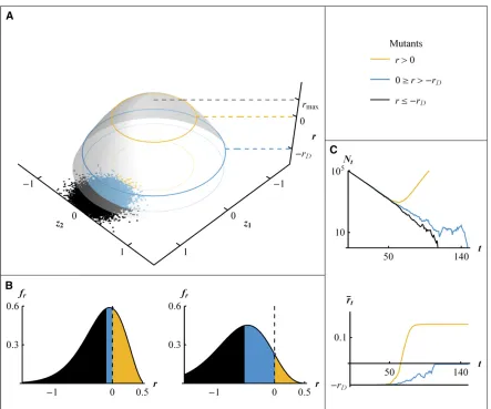
Figure 1 illustrates the rescue process in the FGM. At the onset of stress (t¼0), the optimum shifts abruptly to a new position, such that the mean growth rate becomes negative with 2rD,0 (Figure 1C). Meanwhile, the population size

starts to drop from an initial value N0 (Figure 1C), facing extinction in the absence of evolution. However, one or sev-eral mutants or pre-existing variants may be close enough to the new optimum to have a positive growth rate (“resistant genotypes,”Figure 1, A and B). These may then establish, and ultimately rescue the population (“rescue genotypes”Figure 1, A and B).

Within the context of the FGM, increasing stress level may have different effects, also discussed in Harmand et al.

(2017). First, stronger stress may cause a larger shift in the position of the optimum phenotype, resulting in a larger ini-tial drop infitness (higherrD), as assumed in most models of

also be lower in the new than in the previous environment (reduced environmental quality). Moreover, the mutational parameters (Uandl) may change with stress, causing shifts in evolvability. Note that a change inlmay reflect a change in the phenotypic effects of mutations, of the strength of stabi-lizing selection, or both. For instance, higher stress may re-lease cryptic genetic variance on underlying phenotypic traits (Scharloo 1991; Hermisson and Wagner 2004), or cause in-creased mutation rates via SOS responses in bacteria (Foster 2007). Finally, although less easy to conceptualize, some en-vironments may change the effective dimensionality of the landscape. However, in the present paper, we only consider such changes in dimensionality in the context of rescue from

de novomutations (where it can readily be handled by study-ing the effect of the parametern).

As we will see, all our results can be expressed in terms of

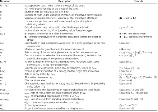
five parameters (N0U;rD;rmax;l;n). Table 1 summarizes all notations in the article.

Strong selection and weak mutation regime

The FGM described in the previous section, produces epistasis forfitness between different mutations, which makes the problem highly intractable in general. To make analytical progress, we assume a regime of strong selection and weak mutation (SSWM; Gillespie 1983), which allows neglect-ing multiple mutants and epistasis. This regime arises when mutation rates are small relative to their typicalfi t-ness effect (as detailed below). In our context, this assump-tion implies that most rescue variants (pre-existing orde novo) are only one mutational step away from the ancestral Figure 1 Evolutionary rescue in Fisher’s geometric model (FGM). In all panels, black refers to deleterious and neutral mutations (2rD$ r), blue to beneficial but not resistant mutations (2rD,r#0), and orange to resistant mutations (r.0), around the dominant genotype of the ancestral population with phenotypezA6¼0:(A) Fitness landscape (FGM) with growth rate r(z-axis) determined by two phenotypic traitsz1andz2:Dots

represent the distribution of random mutant phenotypes around the dominant genotype of the ancestral population. The growth rate of this dominant genotype, in the stressful environment, is2rD;andrmaxis the maximalfitness at the phenotypic optimum. (B) Distribution of growth rates among random mutants arising from the dominant genotype (distribution of mutation effects onfitness) for two decay ratesrD¼0:1 (left) and

rD¼0:5 (right). (C) Dynamics of the population size Nt and meanfitness rt of a population starting from a clone at‒rD¼20:083 at size

N0¼105:The black line represents the case withoutfixation of a beneficial mutation, the blue line the case with extinction in spite of thefixation

of a beneficial, but nonresistant, mutation, and the orange line the case of a rescue. Parameters for the simulations arermax¼1:5;U¼2*1025;

genotype, allowing for two key simplifications. First, with a purely clonal ancestral populations, we can ignore ER by ge-notypes that have accumulated multiple de novomutations. Second, in populations initially at mutation-selection balance, we can consider that all mutations arise from a single domi-nant genotype, optimal in the previous environment. Indeed, in the SSWM regime at mutation-selection balance, most seg-regating phenotypes remain within a narrow neighborhood of the optimum (relative to the magnitude of mutation effects on traits), so the mutation-selection balance is well-approximated by assuming that all mutations originate from the optimum phenotype. This is essentially the House-of-Cards approxima-tion (Turelli 1984) extended to the FGM of arbitrary dimen-sionality (Martin and Roques 2016).

Overall, the SSWM assumption implies that the evolution-ary aspects of ER are entirely determined by a single joint distribution offitness, in the previous and new environment. This distribution corresponds to that of mutants arising from the optimal genotype of the previous environment. We thus apply the results of Martin et al. (2013), to this particular distribution.

Note that the SSWM approximations used in this arti-cle should apply even when multiple single-step mutants

cosegregate (generating“soft selective sweeps,”as detailed in Wilsonet al.2017). Indeed, the probability of ER as com-puted for example in Orr and Unckless (2008) or Martin

et al. (2013) and used here, is one minus the probability that nosinglemutant arises that ultimately causes ER. This means that we ignore ER requiring multiple mutational steps, but allow several single-step rescue mutations to cosegregate. Consistently, our simulations did not show any particular deviation from the theory at very mild stress, where such cosegregation of several single-step mutants is expected.

Maximal mutation rate for the SSWM regime

We conjecture that the SSWM approximation should be accurate below some threshold mutation rate UC; i.e., whenever U,UC¼n2 l=4: Indeed, Martin and Roques

(2016) found that, as long asU#UC;thefitness distribution at mutation-selection balance corresponds exactly to that expected under the House-of-Cards approximation (with a dominant optimal genotype plus its deleterious mutants). Whether this same condition is sufficient for most rescue events to stem from single-step mutations is not justified the-oretically, and was simply tested by extensive stochastic Table 1 Notations

Notation Description Formula

Nt; N0 Nt: population size at timetafter the onset of the stress.

N0: initial population size at the onset of the stress.

U Mutation rate per individual per unit time.

n Number of traits under stabilizing selection, or phenotypic dimensionality.

l Variance of mutational effects: variance of the phenotypic effects of mutations, per trait, in a trait space scaled by the strength of stabilizing selection

dzNð0;lInÞ

Uc Critical mutation rate below which the SSWM regime is valid. UC¼n2 l=4

z n-dimensional vectorz2ℝn_{of (breeding values for) phenotype}

zA;o o:optimal phenotype in a given environment o¼0:new environment

zA:average phenotype of the ancestral population (before the onset of stress)

o¼zA:previous environment

r;s Growth rate (r) and reproductive variance (s) of a given genotype, in the new environment.

Equation (1)

rmax Maximum possible growth rate in the new environment. rð0Þ ¼rmax

rD Rate of decay of the ancestral phenotype zAin the new environment. rðzAÞ ¼rmax2kzAk2=2¼ 2rD

c Cost of a mutation: selective disadvantage of the mutant, relative to the optimal phenotype, in the previous environment.

c¼ kz2zAk2=2

cHðyÞ Harmonic mean of the costcjyamongde novomutations with scaled growth rate yin the new environment

Equation (3)

y Growth rate of a genotype, in the new environment, scaled byrmax. y¼r=rmax2 ½2N;1

fyðyÞ Probability density function ofyamong random single step mutations Equation (2)

yD Rate of decay scaled by rmax: yD¼rD=rmax

cD Alternative measure of yD cD¼2ð

ffiffiffiffiffiffiffiffiffiffiffiffiffiffi 1þyD p

21Þ(Equation (6))

a Effective stress level Equation (6)

ac;rDc Characteristic stress level (ac) or decay rate (rDc) beyond which ER probability

drops below 1=2: Equation (8)

gðaÞ Function driving the dependence of rescue probabilities on stress levels. Equations (7a) and (7b)

vDN;v*DN vDN:rate of rescue fromde novomutations scaled byN0 Equations (5), (7a) and (7b)

v*

DN:corresponding approximation when lrmax

vSV;v*SV vSV :rate of rescue from standing variance scaled byN0 Equations (5) and (10)

v*

SV :corresponding approximation when lrmax

PR Probability of rescue. PR¼12e2N0 vR

simulations. Supplemental Material, Figure S1 in File S1 fur-ther explores the range of validity of this approximation. It shows, in a rescued population, the proportion of wild type, single mutant, double mutant, and so on, as a function of the mutation rate.

Distribution of single-step mutationfitness effects in the new environment

Let sbe the selection coefficient (difference in growth rate), in the new environment, of a random mutant (with phenotype z) relative to its ancestor (with phenotype zA). The distribution of s¼rðzÞ2rðzAÞ ¼rþrD among

ran-dom mutants has a known exact form in the isotropic FGM (Martin 2014; Martin and Lenormand 2015), from which the distribution of growth rates (r¼s2rD)

in the new environment is readily obtained. It proves simpler and sufficient (see Appendix section II, sub-section 2) to consider the scaled (and unitless) growth rate y¼r=rmax2 ½2N;1; such that yD¼rD= rmax2 ½0;þN is the decay rate of the ancestor scaled to the maximum possible growth rate. The scaled growth rates y¼r=rmax have the following probability density

function:

fyðyÞ ¼exp 2 rmaxð2þyD2yÞ l

! rmax

l !n=2

ð12yÞn=221

3

0F1

n

2 ;

_r max

l 2

ð1þyDÞð12yÞ !

Gðn=2Þ ; y2 2N;1

(2)

where0F1ð:; :Þis the confluent hypergeometric function and

GðzÞis the gamma function. In the SSWM regime, this prob-ability density function approximately describes de novo

mutations produced after the onset of stress by the whole population, be it initially clonal or at mutation-selection balance.

Fitness cost of single-step pre-existing mutants in the previous environment

Consider the subset of random mutations, among those that arise from the dominant genotype of the ancestral population, that have a scaled growth rate within the infinitesimal class ½y;yþdy in the new environment. We introduce the conditional random variable cjy;which is the cost, in the previous environment, of a random mutant within this subset (thus, conditional on y). This cost is equal to the negative of the selection coefficient of the mutation relative to the dominant genotype with phenotype zA:More precisely, the cost of a mutant with phenotype z is c¼ kz2zAk2=2 [using Equation (1),

with o¼zA for the previous environment]. Note that, because the mutation-selection balance in the previous environment is fully characterized by relative fitnesses, which do not depend on the maximal growth rate in this

environment, the latter may differ from rmax without

impacting the distribution of the costscjyand our results. Importing results from Martinet al.(2013) for the SSWM regime, the total number of pre-existing variants within the class ½y;yþdy is Poisson distributed with mean

N0 U fyðyÞ=cHðyÞdywhere cHðyÞ ¼1=Ecð1=cjyÞis the

har-monic mean of the costcjyamong mutations with effect y

in the new environment. This conditional harmonic mean depends on the joint distribution of mutation effects on

fitnessðc;yÞacross two environments in the FGM (given in Martin and Lenormand 2015). In our context, the domi-nant genotype of the ancestral population is optimal in the previous environment and far from the optimum in the new environment. In this case, using Equation (9) in Martin and Lenormand (2015), the resulting conditional harmonic mean cHðyÞ takes a tractable form [see Equation (A6) for n$2 and (A8) forn¼1 in Appendix section II, subsection 4 and 5]:

cH

y¼1=Ec

1

cjy

¼

( lvðyÞ ; n¼1

l

evðyÞ_{Eðn21Þ=2vðyÞ}; n$2;

with vy¼rmax l

2þyD22

ffiffiffiffiffiffiffiffiffiffiffiffiffiffiffiffiffiffiffiffiffiffiffiffiffiffiffiffiffiffiffiffi

ð1þyDÞð12yÞ p

2y

(3)

where EkðzÞ ¼ RN

1 e2

zt_=tk _{dt is the exponential integral}

function. In most of the article we focus on the case n$2; when considering ER from standing variance. The distribu-tions of mutation effects on fitness in both the previous [Equation (3)] and the new environment [Equation (2)] can then be integrated to yield the probability of ER, as we show next.

General expression and assumptions for the rescue probability

Extinction occurs when no resistant mutation manages to establish (i.e., to avoid stochastic loss). For compact-ness, we define a rate of rescue vper individual present at the onset of stress (i.e., scaled by N0), such that, fol-lowing Martin et al. (2013), ER probabilities take the general form (similar to that in e.g., Orr and Unckless 2008):

PR¼12e2N0v : (4)

The rate of rescue fromde novomutations alone isvDN(“DN”

for de novo), while that from pre-existing variance alone is vSV(“SV”for standing variants). For a purely clonal

pop-ulation, the rate of rescue isv¼vDN;while for a population initially at mutation-selection balance, it isv¼vDNþvSV

in the SSWM regime assumed here (Martin et al. 2013). Applied to the context of the FGM using Equations (2) and (3), the rates vDNand vSVare given by [see Appendix

vDN¼ U rD

Z1

0

pðyÞfyðyÞdy

vSV¼U R1

0 pðyÞ cHðyÞ

fyðyÞdy;

with pðyÞ ¼12e22yrmax=s

(5)

where cHðyÞ; and Eðn21Þ=2ð:Þ are defined in Equation (3) and pðyÞ is the probability of establishment of a resistant genotype with scaled growth rate y.0 in the new environ-ment.vDNin Equation (5) is simply the average establishment

probability ofde novoresistant mutants times the genomic mu-tation rate, divided by the rate of decay. In previous ER models (e.g., Orr and Unckless 2008; Martinet al. 2013), which we denote“context-independent,”the probability of rescue takes the exact same form as Equation (4). The expressions for the rates of rescue per capita also take a form similar to Equation (5): forde novomutations,vDN¼ U qR = rD;and for

stand-ing variance,vSV ¼U qR = cH;whereqRis the proportion of

rescuers among random mutations [qR¼ R1

0 pðyÞfyðyÞdy in Equation (5)] andcH is again the harmonic mean of the cost

of rescue mutations. The important difference is that in previous models,qRandcHdo not depend on rD;while the

correspond-ing quantities in Equation (5) do depend on the rate of decay, through its effect onfyðyÞandcHðyÞ:

The linearity of ER rates with the mutation rate U(v}U) arises here because of the SSWM regime, where multiple mutations are ignored: it might not hold at higher mutation rates (when U.Uc). As such, Equation (5) makes no

fur-ther assumption than the SSWM regime (U,Uc); it can

easily be evaluated numerically to provide a general test-able theory for rescue probabilities across stress levels, in the FGM. Yet, in order to gain more quantitative/intuitive insight into the effects of stress, we study approximate closed forms for the rates in Equation (5).

Small mutational effects approximation

Although selection is assumed to be strong relative to mutation (U,Uc;SSWM regime), it is still fairly realistic to assume that mutation effects on traits (and thus fitness) are weak relative to the maximal growth rate in the new environment, namely that lrmax: Taking a limit where l=rmax/0; simpler

ex-pressions for Equation (5) are derived in the Appendix section III. With this approximation, single-step resistance mutations are still rare and of large phenotypic effect, in that they pertain to the tail of the mutant phenotype distribution. However, even resistance mutations typically remain far from the optimum in the new environment, so that their scaled growth rate is small: y¼r=rmax1: Overall, mutation effects must fall

within the range: 4U=n2_,lr

maxfor both the SSWM and

the small mutational effects (SME) approximation to apply (see Appendix section III). In the Appendix, we study the con-vergence, asl=rmaxdecreases, of the results from Equation (5)

to their asymptotic limit (Figure S3 and Figure S4 in File S1).

Stochastic simulations of a discrete-time model

We checked the robustness of our assumptions and approx-imations using stochastic simulations, where we tracked the population size and genetic composition of a population across discrete, nonoverlapping generations. The size Ntþ1 of population at generation tþ1 was drawn as a Pois-son number Ntþ1PoissonðNt WÞ;with W ¼er the mean

multiplicative fitness (W¼er_{) and N}

t the population size,

in the previous generation. The genotypes forming this new generation were then sampled with replacement from the previous one with weight Wi¼eri:This is faster and exactly

equivalent to drawing independent Poisson reproductive out-puts for each individual, or genotype. Because of the under-lying assumptions of the simulations, the corresponding analytical approximation for the stochastic reproductive var-iance is si¼s1 (assuming small growth ratesri1).

Mutations occurred according to a Poisson process, with a constant rate Uper capita per generation. Mutation pheno-typic effects were drawn from a multivariate normal distri-bution Nð0;l InÞ; with multiple mutants having additive

effects on phenotype, and theirfitness computed according to the FGM [Equation (1)].

Rescue probability was estimated by running 1000 repli-cate simulations until either extinction or rescue occurred. A population was considered rescued when it reached a popu-lation size Ntand mean growth ratertsuch that its ultimate

extinction probability, if it were monomorphic, would lie below 10212_{[expð22 Nt r}

tÞ,10212]. This is a conservative

criterion: oncerthas become positive, we expect it to remain

so, yielding further increases in population size and thus fur-ther decreasing the probability of future extinction. We checked on a subset of simulations that the above procedure gave the same rescue probabilities as obtained in simulations performed until the population rebounded back to its (large) initial size N0.

For rescue from populations at mutation-selection balance, eight replicate initial equilibrium populations were generated, each by starting from an optimal clone and running the same algorithm with fixed population size (Nt¼106) until the

mean growth rate had visually stabilized to a fixed value (close to its theoretical equilibrium value req¼rmax2U,

for U,Uc) for more than 1000 generations. Then the

opti-mum was shifted by ffiffiffiffiffiffiffiffiffiffiffiffiffiffiffiffiffiffiffiffiffiffiffiffiffi2ðrDþrmaxÞ p

phenotypic units, and 1000 replicate ER simulations were performed (same algo-rithm as forde novorescue), from each of the eight replicate equilibrium populations.

All simulations and mathematical derivations were per-formed inMATHEMATICA v. 9.0(Wolfram Research 2012).

Data availability

code (MATHEMATICA v. 9.0Wolfram Research 2012). Sup-plemental material available at Figshare: https://doi.org/

10.25386/genetics.5975008.

Results

The ER rates in Equation (5) are analytical but only implicit functions of the model parameters. In a SME limit, they take simpler closed forms (indicated by a “*”). As we will see below, these simpler forms mostly depend on the following two compound variables, which summarize the various ef-fects of stress on thefitness landscape:

cD¼2

ffiffiffiffiffiffiffiffiffiffiffiffiffiffiffiffiffiffiffiffiffiffiffiffiffi

1þrD=rmax p

21

a¼ c2D rmax

4 l

: (6)

BothcDandaincrease with the decay rate rD;decrease with

increasing peak height rmax;and are independent of n:The parameter a further increases with decreasing variance of mutational effectsl:We can already see howaqualitatively reflects an“effective stress level”: stress is harder to cope with if decay rate is larger, the maximum growth rate is lower, and mutation effects are smaller.

Rescue from de novo mutations

Under the SME approximation and in the SSWM regime (4 U=n2_,lr

max) the rate of de novorescue [Equation (5)], converges to [Equation (A12) in the Appendix]:

vDN

l rmax

v* DN¼U

ð1þcD=2Þð12nÞ=2

1þcD=4 gðaÞ; (7a)

v*

DN /

cD=2/0

U gðaÞ; (7b)

with

gðaÞ ¼ effiffiffiffiffiffiffiffiffi2a p a

p 2erfc ffiffiffipa;

where erfcð:Þis the complementary error function. Equation (7b) gives the approximate closed form of Equation (7a) for mild stressðcD=2 / 0Þ:Note that this approximation con-verges faster (with decreasing cD) with fewer dimensions,

due to the faster vanishing of the factorð1þcD=2Þð12nÞ=2(in the limit n¼1 it vanishes for all cD). We now discuss the

biological implications of these expressions.

Effect of FGM parameters on rescue

The partial derivatives of v*

DNin Equations (7a) and (7b) with

respect to the FGM parameters (rD;rmax;l;n) quantify the sen-sitivities of ER probability to each of them (Appendix section III, subsection 4). First, note thatgð:Þis a strictly decreasing function of a:When n.1 and with mild stress (cD2), Equation (7b)

applies andvDN U gðaÞ:ER then becomes less likely with a

higher decay rate rD;a lower peakrmaxand a smaller variance of

mutational effectsl;and is independent of dimensionalityn:For stronger stress levels, Equation (7a) applies: these qualitative dependencies to the parameters still hold, except that ER proba-bility now decreases with increasing dimensionality.

Sharp drop of ER probability with stress levels

Figure 2 shows the agreement between simulations (stochas-tic discrete-time demographic model, seeMethods) and the analytical expressions in Equations (5), (7a), and (7b), over a wide range of stress levels (quantified by rD), and for two

values ofrmax andU (Figure S3 in File S1 further explores

the range of validity of the approximation). Interestingly, ER probability drops sharply with stress levels (with decay rate

rD here), which is well captured by the term gðaÞ alone

[Equation (7b), dashed red lines in Figure 2]. This drop is much more pronounced than in a context-independent model (gray lines in Figure 2), where stress does not affect the distribution of mutation effects. The difference between Figure 2 Rescue probability fromde novomutations. The ER probability as a function of stress levels, expressed as the initial mean decay rate of the population, is given for various values of the mutation rateU¼1023 _U

context-independent models and the FGM is that, in the lat-ter, increased stress implies both faster decay (as in the former), and fewer and weaker resistance mutations. In the FGM, these effects on the properties of rescue mutations are the main drivers of ER probabilities across stress levels.

Composite parameter adescribing an effective stress level

The results in Equations (6), (7a), and (7b) suggest that a single composite parameter [ain Equation (6)] can capture the various ways in which stress may alter the parameters of thefitness landscape, that is,fitness peak heightrmax; vari-ance of mutational effectsl;or distance to the optimum rD:

We denote this parameter the“effective stress level.”In Fig-ure 2, considering the effect of stress only via a[Equation (7b)] is equally accurate as using the more complex Equation (7a), or the numerical computation from Equation (5).

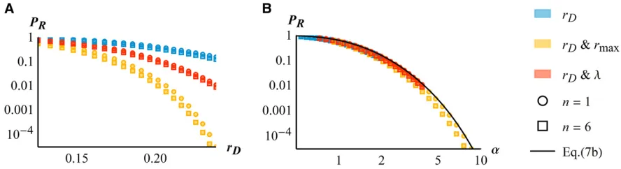
This simplification is further illustrated in Figure 3, where we use exact numerical computations from Equation (5) to explore different possible effects of stress. Regardless of whether stress affects only the maladaptation of the ancestral clone (rD;blue symbols), or also the quality of the environment (joint change in

rD and rmax; orange symbols) or the variance of mutational

effects (joint change in rD and l; red symbols), its effect on

the rescue probability is accurately predicted by a(Figure 3B, black line). As predicted by Equation (7b), the relationship be-tween rescue probability andais approximately independent of dimensionality (compare circles n¼1 and squares n¼6 in Figure 3B). We also note that Equation (7b) slightly overesti-mates the“exact”numerical computations of the ER probability from Equation (5), so it provides a conservative bound when considering the control of resistant pathogens.

Characteristic stress level

Figure 2 shows that ER drops from highly likely to highly unlikely around a “characteristic stress level,” which can be characterized analytically (as detailed in the Appen-dix section IV, subsection 1). Consider the set of values

of parameters ðN0;U;rmax;rD;l;and nÞ for which the rescue probability is of given value p2 ½0;1: From Equa-tion (7b), this corresponds to the set ðrmax;rD;lÞ for which a¼g21_{½2logð12pÞ=N}

0U. Using the approximation

gðaÞ a23=2_e2 a_=ð2pffiffiffiffi_{pÞ [from Equations (7a) and (7b)} with a1], the correspondingacan be derived explicitly [Equation (A17)]. In particular, forp¼1=2;the characteris-tic stress levelacat which the ER probability is 1=2 is

[Equa-tion (A19) in the Appendix]:

ac N0U1

g21

logð2Þ

N0U

N0U1

0:9logðN0UÞ22:7 : (8)

Under the conditions of the SME approximation (detailed in

Methods), Equation (8) applies for large N0U (approximately when N0U$5:104), a necessary condition for this equation to be self-consistent (detailed in Appendix section IV, subsection 2). The characteristic stress level ac that a population can

typically withstand increases only log-linearly with popula-tion size and mutapopula-tion rate. Consider the characteristic decay rate rc

Dfor which the rescue probability isPR¼1=2;i.e., the

decay rate that populations can overcome half of the times. From Equation (8) withac}ðrcDÞ

2

[Equation (6)], this decay rate is rc

D}

ffiffiffiffiffiffiffiffiffiffiffiffiffiffiffiffiffiffiffi

logðN0UÞ p

for large N0U:For comparison, we would have rc

D¼qRN0U=logð2Þ;which is linear in N0U;in a context-independent model where the proportionqRof

ran-dom mutations causing a rescue is independent of rD:The dif-ference in the effect of N0U on rescue probability thus stems from the strong nonlinearity (i.e., sharp drop) of rescue proba-bility with stress level (decay rate) under the FGM. In the FGM, overcoming a given environmental harshness requires much more mutational input than in a context-independent model.

Characteristic stress window

It is also important to predict how sharply the ER probability drops around the characteristic stress level. This drop can be characterized by a“characteristic stress window”of aover which the ER prob-ability drops from 75 to 25%. The widthDaof this window can be Figure 3 The effective stress level. Rescue probability for clonal populationsvs.initial decay raterD(A) or the effective stress levela(B). In both panels the axes are in logarithmic scale, symbols show Equation (5) and colors refer to different effects of increased stress level: blue symbols show onlyrD increasing (withrmax¼1:5 andl¼0:005Þ;orange symbolsrDincreasing andrmax decreasing linearly withrD(according tormax¼1:525rD;with

l¼0:005) and red symbolsrDincreasing andldecreasing linearly withrD(according tol¼0:00521022 rD;withrmax¼1:5). In each case, the results

for bothn¼1 (circles) andn¼6 (squares) are shown. The black plain line on the right panel gives the result from Equation (7b): a single composite measure of stressðaÞapproximately captures the impact of stress-induced variations in the various parametersðrD;rmax;l;nÞ:Other parameters are

scaled by the value of the characteristic stress level ac;to get a scale-free measure of its steepness (i.e., how sharp the drop in ER probability is, relative to the stress level around which it occurs). This gives [from Equation (A20) in the Appendix]:

Da ac N0U1

1 1þ0:7ac :

(9)

The widthDaincreases with increasing N0U until it saturates (at 1:5) (see Appendix section IV, subsection 3 for further details). However, when scaled by the center of the window (ac),

the width of this scaled characteristic stress window drops below 1 asacincreases [and hence with increasingN0U;from Equation (8)]. This result shows formally that the drop in ER probability with increasing stressagets proportionally sharper (relative to the position where it occurs) as N0Uincreases, but this is entirely driven at largeN0U by shifts of a window with constant absolute width. This is illustrated in Figure 4, which also shows the accuracy of Equation (9) compared to“exact” numer-ical computations from Equation (5) [as expected, the exact re-sult deviates from Equation (9) for smaller N0U].

Interestingly, Equation (9) provides a scale-free measure that may be compared across experiments, as it only depends on the genomic mutational input N0U(via ac). However, like all

results so far, Equation (9) only considers ER fromde novo

mutation. We now turn to ER from standing genetic variation.

Rate of rescue from a population at mutation-selection balance

In the SSWM regime, and for a population at mutation-selection balance in the previous environment, each rescue event can be tracked back to either a pre-existing variant, or ade novomutation (Orr and Unckless 2008, 2014; Martinet al.2013). The proportion

fSV of rescue events caused by standing variance is then simply

given by fSV ¼vSV=ðvSVþvDNÞ:A simple expression can be

obtained again under the SME forn$2 [see Equation (A21) in the Appendix], but the approximation (f*

SV) now further requires

that decay rates are not vanishingly small (lrmax c2D=4).

fSV¼ vSV

vSVþvDN l rmaxc2D=4

f* SV¼

1þcD=4

e=cDþ1þcD=2

where e¼l n21 2 rmax;

(10)

where cDis defined in Equation (6).

Equation (10) captures the main features of how standing variance contributes to ER across (nonvanishing) stress levels (here, decay rate). Contrary to context-independent models, this contribution changes nonmonotonically with increasing stress level (Figure 5). At very mild decay raterD;rescue relies on mild-effect mutations. The cost of such mutations—and hence their frequency before stress—is roughly independent ofrD(Martin and Lenormand 2015), while their rate of

pro-duction by de novo mutation decreases as 1=rD

(demo-graphic effect), so the contribution of standing variance to

ER increases with rD at smallrD:In contrast at large stress

levels, rescue stems from strong effect mutations. These mu-tations pay a substantial“incompressible cost”before stress that increases faster thanrD(Martin and Lenormand 2015),

while their rate ofde novoproduction still decreases as 1=rD;

so the contribution of standing variance to ER decreases with

rDat largerD:In the limit of very large yD;the distance

be-tween the two optima is very large and makes the most of both the cost and decay rate, so that cHðyÞ rDfor all

mu-tations. Hence,de novomutations and standing variants con-tribute equally to ER in this limit (fSV/1=2).

These different behaviors are illustrated in Figure 5, show-ing the variation of fSV over a very wide range of scaled

decay rates yD. The limit fSV/f*SV in Equation (10)

pro-vides a fairly accurate approximation across the full range of stress levels. The limits when yD/0 and yD/Nare in

fact of limited biological interest, as they correspond to stress levels where ER becomesde factocertain or impossible, re-spectively. When focusing on the more biologically relevant range corresponding to the characteristic stress window, which occurs near the peak infSVin Figure 5 (see Appendix

section IV, subsection 4), the variation offSV across stress

levels becomes negligible. As illustrated in Figure 6B, fSV

remains close to 12pffiffiffie[see Appendix Equation (A22)] as

yDvaries over a range where ER probabilities span several

orders of magnitude (see Appendix Section IV subsection 5). Note that this behavior arises when stress only shifts the optimum (effect on rD), but does not affect peak height

(rmax) or the variance of mutational effects (l).

Therefore the rate of rescue in the presence of standing variance is approximately proportional to that with onlyde novo mutation, with proportionality constant largely inde-pendent of the decay rate:

v¼vDNþvSV v*DN= ffiffiffi e

p

; (11)

where e is defined in Equation (10). The rough constancy of fSV also means that all the results obtained previously

for ER from de novo mutations apply in the presence of Figure 4 Scaled width of the characteristic stress windowDa=acvs.the population-scale mutation rateN0U:The dots are obtained by numerical

standing variance, when stress only shifts the optima (as long asn$2Þ.

The ER probability profile across stress levels (shown in Figure 6A) is the same as that from de novo muta-tions alone (Figure 2), but with a higher characteristic stress [ac

N0U1

0:9logðXÞ22:7 from Equation (8) with

XN0U= ffiffiffi e

p

]. Moreover, when considering the contribu-tion from standing variance, the difference between the FGM and context-independent models (gray line on Figure 6A) is striking. Indeed in the latter, the ER rate from standing variance (vSV) is independent of the decay rate, hencePR

satu-rates with stress to a constant value 12expð2 N0 U qR=cHÞ;

where all ER events stem from standing variance.

Finally, note that when considering rescue from preexisting variance, U may change across environments, from UP (for

previous) toUN (for new). For example, a stress-induced

in-crease in DNA copy error would yield UN.UP:Accounting for

such shifts in mutation rate at the onset of stress, the total ER rate simply becomes v v*

DNð1þUP=UNð12pffiffiffieÞ=pffiffiffieÞ [from

Equation (11)].

Discussion

Main results

We investigated the persistence of a population of asexual organisms under an abrupt environmental alteration. We assumed that this stress causes a shift in a multidimen-sional fitness landscape with a single peak (FGM), which the population must “climb”to avoid extinction. In such a landscape, faster population decline (due to stress-induced increase in the decay rate rD) necessarily means that

resis-tance mutations are fewer, have lower growth rates in the presence of stress, and higher costs in its absence. We believe that this constraint, not included in previous studies, adds a key element of realism to ER models. In our model, variation in stress levels may affect the landscape in various ways: shifting the optimum, changing the peak height, or altering the phenotypic scale of mutations (or the strength of

stabi-lizing selection). Under a SSWM regime and assuming SME, all these effects of stress on the distribution of mutationfi t-ness effects are approximately captured by the variation, across stress levels, of a single composite parameter a;which is approximately independent of the dimensionality of the organism (number of orthogonal traits under selection). The probability of ER drops sharply with this effective stress level, more so than in previous ER models where the rate of population decline is decoupled from the input of resistant mutations. The characteristic stress window over which this drop occurs only depends on the initial population size

N0 and genomic rate of mutationU:As N0Ugets large, the characteristic stress window reaches an asymptotic width [Dain Equation (9)] while its center [the characteristic stress levelacin Equation (8)] shifts toward higher values,

approx-imately as logðN0UÞ:

When standing variance is available (population at muta-tion-selection balance before stress), its contribution to ER is dominant, and approximately constant across a wide range of stress levels that encompasses the characteristic stress window.

In Table 2, we summarize how these features compare to properties of previous ER models. We consider only the situ-ation where stress shifts the position of the optimum, affect-ingrD(as in previous models), because other effects of stress

we investigate here (rmaxand l) are not treated in previous models.

Genetic basis of ER patterns across environments

Our model allows identification of three ranges of stress levels that yield different eco-evolutionary patterns, despite all leading to extinction in the absence of evolution. First, at low stress levels (aac), although evolutionary change is

required for persistence and demographic dynamics typical of ER may be observed (decay/rebounce), extinctions are de factoundetectable (ER is pervasive,PR1). In this regime,

we expect several resistance mutations to establish and cose-gregate (frequent “soft sweeps” as in Wilson et al. 2017). Their number is predictable (N0vR), but the ultimate

com-position of the population in asexuals will depend on more complex clonal interference dynamics. Second, at intermediate stress levels [a¼OðacÞ], small variation in

stress conditions has large impact on the probability of population survival. Over this range, PR1=2 so the

expected overall number of rescue mutations in the popula-tion is less than one [N0vR 2logðPRÞ ¼0:7]. Therefore, “hard sweeps”(including from standing variation) should be the most frequent: a single mutation typically establishes and rescues the population. Finally, at higher stress levels (aac), very few populations overcome the imposed stress,

and when they do it is typically through a hard sweep (N0vR1).

Estimating parameters and testing the model

Studies on the emergence of resistance to controlled stress (e.g., antibiotics, fungicides, and chemotherapy in cancer), Figure 5 Relative contribution of standing genetic variation to ER. The

proportion of ER from standing variance is shown across scaled decay rates yD: The numerical computation forfSV [using Equations (5) and (10)], for two values of rmax¼0:1 (blue) andrmax¼0:7 (orange), is com-pared to the approximate f*

especially in microbes, can generate a set of estimates of PR

(the probability of resistance emergence), across stress levels. In general, to test (or use) predictions from ER models, it is critical to empirically relate physical measures of stress level (e.g., concentrations, temperatures, salinities,etc.) with de-mographic measures (e.g., decay rates). If we assume that the main effect of stress is to shift optimum positions, given a set of measurements of rD (“dose-kill curves;” Regoes et al.

2004), the change in ER probability with stress can be pre-dicted via Equations (7a) and (7b). This simple scenario of optimum shifting is the one that is considered by most of the literature on evolutionary ecology across environmental gra-dients, so it would seem natural to test itfirst. Furthermore, this scenario has received empirical support from an analysis of a few experimental studies of distribution of mutation effects onfitness across stress levels (Martin and Lenormand 2006b). However, these studies used mild stresses, which reduce growth without causing population decay. A more recent study on bacteria facing lethal doses of antibiotics,

i.e., in the presence of decay (Harmandet al.2017), suggests that factors other than the position of the optimum may also change with stress (l;rmax;n). Estimating these extra param-eters across environments can be challenging. The variance of mutational effectsland the dimensionalityncan be esti-mated byfitting the distributions of single random mutation effects on fitness (Martin and Lenormand 2006b; Perfeito

et al.2014), in a single environment if it is to be assumed constant, or in each environment otherwise. The maximal growth rate in the stress could be measured on lines well-adapted to the environment considered.

The effective stress levelais also amenable to empirical measurement and circumvents the issue of measuring joint changes in ðrD;rmax;lÞwith stress. Consider a set of PR

esti-mates across a range of empirically controlled stress levels, and some knowledge of the genomic (non-neutral) mutation rate (e.g., as estimated by mutation accumulation experi-ments) of the species and environment under study (U). The initial population size N0is easily controlled by the ex-perimenter. Then Equation (7b) suggests a simple estimator of ain each environment:ba¼g21_ð2logð12P

RÞ=N0UÞ: Finally, it is also possible to circumvent the problem of stress-induced variation in the parameters of thefitness landscape by considering multiple genetic backgrounds, ina single environment. Each background would have a given measurable decay rate rD;

and other parameters (l;rmax;n;U) would be heldfixed; while

l;nandUmay change with the genetic background, this seems less likely than with the environment. The isotropic FGM assumes a strict equivalence between shifts in optima (multiple environ-ments) from a given ancestor phenotype (single genetic back-ground), and shifts in ancestor phenotypes (multiple genetic backgrounds) with afixed optimum (single environment). The model could thus be applied and tested in this context. This could yield useful insights into the effect of epistasis (background de-pendence) on resistance emergence, an issue of notable impor-tance when considering the fate of horizontally transferred resistance or multidrug resistance (as discussed in Wong 2017)

Potential implications for resistance management

Our results suggest that stress levels have a strongly nonlinear impact on ER probabilities (Figure 2), at least in the context of abrupt environmental changes, in asexuals. This context may be particularly relevant to the chemical treatment of patho-gens (cancer therapy, antivirals, antibiotics, fungicides, her-bicides,etc.). In particular, the nonlinear impact of stress on ER, if empirically confirmed, can provide insights regarding the optimization of treatment regimens or the quantification Figure 6 ER probability in the presence of standing genetic variation. In each panel, stress only affects the decay raterD(shifting optimum). In both panels, blue solid lines show the theory forde novoand standing variance (“DN”+“SV”) computed numerically [Equation (5)] and the gray lines correspond to an equivalent theory without the FGM (named context-independent model as described in theMethodssection,“CI”) modified from Orr and Unckless (2008). This last model was computed using afixed proportion of resistant mutations equal to the one in Equation (5) for a rescue probability of 0:5 (which explains why the two curves cross exactly atPR¼0:5). The dashed red line gives the simpler expression for the overall rescue rate: v v*

DN= ffiffiffi

e

p

:[Equation (11)] withegiven in Equation (10) and v*

DNby Equations (7a) and (7b). (A) ER probability in the presence of standing genetic variation as a function ofrD:The dots give the results from simulations. (B) Proportion fSVof rescue from standing variance as a function of rD: The black dashed-line give the approximate theory from Equation (10) and the dashed red line maxðf*

SVÞ 12 ffiffiffi

e

p

of the effect of poor treatment adherence on resistance emer-gence (e.g., in HIV, Harriganet al.2005). Our results point to the risk that even a slight lowering of drug doses (below prescribed treatment levels) could radically change the out-come of the treatment (making itde factoinefficient). On the contrary, a slight increase in prescribed doses could some-times prove sufficient to allow efficient eradication.

Limits and possible extensions

Density-dependence and competitive release: Our model ignores density dependence, but some form may be easily introduced by considering a single density dependence co-efficient (common to all genotypes) and using logistic diffu-sion approximations (Lambert 2005). This would potentially allow for“competitive release”(Readet al.2011), whereby higher stresses may favor the emergence of resistance by rapidly depleting the sensitive wild-type population, thus re-leasing limiting resources for resistant genotypes. Previous models on competitive release assumed that the number of standing resistant mutants is independent of stress level (Read et al. 2011; Day and Read 2016). In this case, stress mostly limitsde novorescue mutation, with limited impact on the contribution from standing variance. On the contrary, the FGM imposes a similar drop, with stress, in the rate of rescue fromde novoand preexisting mutants. The positive effects of competitive release on ER probability may thus be less impor-tant, in the FGM, than predicted from these previous models. Note however that more generally, the effect of density depen-dence on ER is more safely investigated by accounting explicitly for the effect of stress on the density-independent intrinsic rate of increase on the one hand (as done here in a density-inde-pendent model),vs.on the competition component on growth (e.g., carrying capacity) on the other hand, than by compound-ing their effects into an overall density-dependent decay rate (e.g., Chevin and Lande 2010). This would require modeling the effect of stress on both the intrinsic rate of increase and the competition component, possibly through a landscape with twofitness functions, describing each component.

Anisotropy and parallel evolution in drug resistance:The present model is isotropic: all directions in phenotype space are equivalent (in terms of mutation and selection). In con-trast, module-dependent anisotropy (where particular genes mutate along favored directions) can lead to substantial parallel evolution in the FGM (Chevinet al.2010). Parallel

evolution of resistance, whereby some (portions or sets of) genes contribute most of the resistance mutations, is often observed among drug-resistance alleles, and can increase with stress (Harmandet al.2017), contrary to parallel evo-lution in a growing population, which is expected to decrease with increasing maladaptation (Chevin et al. 2010). Al-though not explored here, we conjecture that our model may accommodate mild anisotropy. Indeed, mild anisotropy (even environment-dependent) might have limited impact. If mutational covariances between traits merely“turn,” “shrink” or“expand”the phenotypic mutant cloud, this would approx-imately amount to a mere change inlin an equivalent iso-tropic landscape (Martin and Lenormand 2006a; Martin 2014). However, a particular form of strong anisotropy may also arise where mutant phenotypes (in a given module) spread along a single favored direction (Martin 2014). Only this level of anisotropy would generate clear parallel evolu-tion, and it will likely require implementing a fully anisotropic model.

High mutation rates:Our results relied on a SSWM approx-imation. When the mutation rate is higher (e.g., viruses or mutator bacterial strains), multiple mutants must be accounted for as a source of ER. These can in principle be introduced in the framework used here (Martinet al.2013), but, especially when applied to the FGM, the results quickly become intractable. Alternative population genetics assump-tions would then have to be used, but this is beyond the scope of the present work.

Conclusion

Recently, the FGM has received renewed interest for its ability to provide testable, quantitative, and often accurate predictions regarding patterns of mutation effects on fitness, across various species and contexts (Tenaillon 2014). The present model is an attempt to extend its scope to model the evolu-tion of resistance to stress. We hope that future experimen-tal tests will evaluate its accuracy and potential to tackle various pressing applied issues.

Acknowledgments

We thank the editor Joachim Hermisson and the reviewers for their help in improving this manuscript. In particular we Table 2 Main results of“context-independent”modelsa_{and the present model (FGM) when stress only affectsr}

D(only shifts the optimum

position in our model)

Context-Independent Model FGM Rescue Model

Impact of decay raterD vD N}rD21; vSV¼constant v}e2r

2

D r23

D (1)

Impact of mutational inputN0U v}N0 U v}N0 U

“Characteristic decay rate”(rc

D) for DN rescuevs. N0 U rcD}N0 U rcD}

ffiffiffiffiffiffiffiffiffiffiffiffiffiffiffiffiffiffiffiffiffiffi logðN0 UÞ p

Relative contribution of standing variance to ER Increases withrDfSVrD=rDþc Stable withrDfSV12pffiffiffie

When the dependence to the parameters is given for the overall rate of rescuev;it applies to both the rate of rescue fromde novomutationsvDNand from pre-existing variancevSV:(1) derived from the approximate expressiongðaÞ a23=2e2a=ð2pffiffiffiffipÞ:

thank Michael Kopp for extensive and very useful comments on our manuscript. This work benefited from discussions with S. Gandon, R. Gomulkiewicz, O. Tenaillon, F. Débarre, and L. Roques. This work was supported by the French Min-istry of Higher Education, Research and Innovation (MESRI allocation doctorale to Y.A.), Agence Nationale de la Recherche (ANR-13-ADAP-0016 “Silentadapt”to G.M. and ANR-13-ADAP-0006 “MeCC” to O.R.) and European Re-search Council (ERC-2015-STG-678140-FluctEvol to L.-M.C.). This is ISEM publication ISEM 2018-032.

Literature Cited

Agrawal, A. F., and M. C. Whitlock, 2010 Environmental duress and epistasis: how does stress affect the strength of selection on new mutations? Trends Ecol. Evol. 25: 450–458.

Alexander, H. K., G. Martin, O. Y. Martin, and S. Bonhoeffer, 2014 Evolutionary rescue: linking theory for conservation and medicine. Evol. Appl. 7: 1161–1179.

Bell, G., 2017 Evolutionary rescue. Annu. Rev. Ecol. Evol. Syst. 48: 605–627.

Bijlsma, R., and V. Loeschcke, 2005 Environmental stress, adap-tation and evolution: an overview. J. Evol. Biol. 18: 744–749. Burger, R., and M. Lynch, 1995 Evolution and extinction in a

changing environment: a quantitative-genetic analysis. Evolu-tion 49: 151.

Carlson, S. M., C. J. Cunningham, and P. A. H. Westley, 2014 Evolutionary rescue in a changing world. Trends Ecol. Evol. 29: 521–530.

Charmantier, A., and D. Garant, 2005 Environmental quality and evolutionary potential: lessons from wild populations. Proc. Biol. Sci. 272: 1415_–1425.

Chevin, L.-M., 2011 On measuring selection in experimental evo-lution. Biol. Lett. 7: 210_–213.

Chevin, L.-M., and R. Lande, 2010 When do adaptive plasticity and genetic evolution prevent extinction of a density-regulated population? Evolution 64: 1143–1150.

Chevin, L.-M., G. Martin, and T. Lenormand, 2010 Fisher’s model and the genomics of adaptation: restricted pleiotropy, heterog-enous mutation, and parallel evolution. Evolution 64: 3213– 3231.

Davies, J., and D. Davies, 2010 Origins and evolution of antibiotic resistance. Microbiol. Mol. Biol. Rev. 74: 417_–433.

Day, T., and A. F. Read, 2016 Does high-dose antimicrobial che-motherapy prevent the evolution of resistance? PLoS Comput. Biol. 12: e1004689.

De Visser, J. G. M., and D. E. Rozen, 2005 Limits to adaptation in asexual populations. J. Evol. Biol. 18: 779–788.

Drlica, K., 2003 The mutant selection window and antimicrobial resistance. J. Antimicrob. Chemother. 52: 11–17.

Feller, W., 1951 Diffusion processes in genetics, pp. 227–246 in Proceedings of the Second Berkeley Symposium on Mathematical Sta-tistics and Probability. University of California Press, Berkeley, CA. Foster, P. L., 2007 Stress-induced mutagenesis in bacteria. Crit.

Rev. Biochem. Mol. Biol. 42: 373–397.

Gillespie, J. H., 1983 Some properties offinite populations expe-riencing strong selection and weak mutation. Am. Nat. 121: 691–708.

Gomulkiewicz, R., and R. D. Holt, 1995 When does evolution by natural selection prevent extinction? Evolution 49: 201. Gomulkiewicz, R., R. D. Holt, M. Barfield, and S. L. Nuismer,

2010 Genetics, adaptation, and invasion in harsh environments. Evol. Appl. 3: 97_–108.

Gonzalez, A., and G. Bell, 2013 Evolutionary rescue and adapta-tion to abrupt environmental change depends upon the history of stress. Philos. Trans. R. Soc. Lond. B Biol. Sci. 368: 20120079. Gonzalez, A., O. Ronce, R. Ferriere, and M. E. Hochberg, 2013 Evolutionary rescue: an emerging focus at the intersec-tion between ecology and evoluintersec-tion. Philos. Trans. R. Soc. B Biol. Sci. 368: 20120404.

Harmand, N., R. Gallet, R. Jabbour-Zahab, G. Martin, and T. Le-normand, 2017 Fisher’s geometrical model and the mutational patterns of antibiotic resistance across dose gradients. Evolution 71: 23–37.

Harrigan, P. R., R. S. Hogg, W. W. Y. Dong, B. Yip, B. Wynhoven et al., 2005 Predictors of HIV drug-resistance mutations in a large antiretroviral-naive cohort initiating triple antiretroviral therapy. J. Infect. Dis. 191: 339_–347.

Hermisson, J., and G. P. Wagner, 2004 The population genetic theory of hidden variation and genetic robustness. Genetics 168: 2271_–2284.

Hietpas, R. T., C. Bank, J. D. Jensen, and D. N. A. Bolon, 2013 Shifting_fitness landscapes in response to altered envi-ronments. Evolution 67: 3512_–3522.

Hoffmann, A. A., and J. Merilä, 1999 Heritable variation and evo-lution under favourable and unfavourable conditions. Trends Ecol. Evol. 14: 96–101.

Hoffmann, A. A., and P. A. Parsons, 1997 Extreme Environmental Change and Evolution. Cambridge University Press, Cambridge, New York.

Koehn, R. K., and B. L. Bayne, 1989 Towards a physiological and genetical understanding of the energetics of the stress response. Biol. J. Linn. Soc. Lond. 37: 157–171.

Kopp, M., and S. Matuszewski, 2014 Rapid evolution of quantita-tive traits: theoretical perspecquantita-tives. Evol. Appl. 7: 169–191. Lambert, A., 2005 The branching process with logistic growth.

Ann. Appl. Probab. 15: 1506–1535.

Lindsey, H. A., J. Gallie, S. Taylor, and B. Kerr, 2013 Evolutionary rescue from extinction is contingent on a lower rate of environ-mental change. Nature 494: 463–467.

Lynch, M., W. Gabriel, and A. M. Wood, 1991 Adaptive and de-mographic responses of plankton populations to environmental change. Limnol. Oceanogr. 36: 1301_–1312.

MacLean, R. C., G. G. Perron, and A. Gardner, 2010 Diminishing returns from bene_ficial mutations and pervasive epistasis shape the_fitness landscape for rifampicin resistance in Pseudomonas aeruginosa. Genetics 186: 1345_–1354.

Martin, G., 2014 Fisher_’s geometrical model emerges as a prop-erty of complex integrated phenotypic networks. Genetics 197: 237–255.

Martin, G., and T. Lenormand, 2006a A general multivariate extension of Fisher’s geometrical model and the distribution of mutationfitness effects across species. Evolution 60: 893– 907.

Martin, G., and T. Lenormand, 2006b Thefitness effect of muta-tions across environments: a survey in light offitness landscape models. Evolution 60: 2413–2427.

Martin, G., and T. Lenormand, 2015 Thefitness effect of muta-tions across environments: Fisher’s geometrical model with mul-tiple optima. Evolution 69: 1433–1447.

Martin, G., and L. Roques, 2016 The nonstationary dynamics of fitness distributions: asexual model with epistasis and standing variation. Genetics 204: 1541–1558.

Martin, G., S. F. Elena, and T. Lenormand, 2007 Distributions of epistasis in microbes fit predictions from a fitness landscape model. Nat. Genet. 39: 555–560.

Moser, C., and G. Bell, 2011 Genetic correlation in relation to differences in dosage of a stressor. J. Evol. Biol. 24: 219–223. Orr, H. A., and R. L. Unckless, 2008 Population extinction and the

genetics of adaptation. Am. Nat. 172: 160–169.

Orr, H. A., and R. L. Unckless, 2014 The population genetics of evolutionary rescue. PLoS Genet. 10: e1004551.

Perfeito, L., A. Sousa, T. Bataillon, and I. Gordo, 2014 Rates of fitness decline and rebound suggest pervasive epistasis. Evolu-tion 68: 150–162.

Read, A. F., T. Day, and S. Huijben, 2011 The evolution of drug resistance and the curious orthodoxy of aggressive chemother-apy. Proc. Natl. Acad. Sci. USA 108: 10871_–10877.

Regoes, R. R., C. Wiuff, R. M. Zappala, K. N. Garner, F. Baquero et al., 2004 Pharmacodynamic functions: a multiparameter ap-proach to the design of antibiotic treatment regimens. Antimi-crob. Agents Chemother. 48: 3670–3676.

Remold, S. K., and R. E. Lenski, 2001 Contribution of individual random mutations to genotype-by-environment interactions in Escherichia coli. Proc. Natl. Acad. Sci. USA 98: 11388–11393. Remold, S. K., and R. E. Lenski, 2004 Pervasive joint influence of

epistasis and plasticity on mutational effects in Escherichia coli. Nat. Genet. 36: 423–426.

Samani, P., and G. Bell, 2010 Adaptation of experimental yeast populations to stressful conditions in relation to population size. J. Evol. Biol. 23: 791–796.

Scharloo, W., 1991 Canalization: genetic and developmental as-pects. Annu. Rev. Ecol. Syst. 22: 65–93.

Sgrò, C. M., and A. A. Hoffmann, 2004 Genetic correlations, tradeoffs and environmental variation. Heredity 93: 241–248.

Tenaillon, O., 2014 The utility of Fisher’s geometric model in evolutionary genetics. Annu. Rev. Ecol. Evol. Syst. 45: 179– 201.

Trindade, S., A. Sousa, and I. Gordo, 2012 Antibiotic resistance and stress in the light of Fisher’s model. Evolution 66: 3815– 3824.

Turelli, M., 1984 Heritable genetic variation via mutation-selec-tion balance: Lerch’s zeta meets the abdominal bristle. Theor. Popul. Biol. 25: 138–193.

Uecker, H., and J. Hermisson, 2016 The role of recombination in evolutionary rescue. Genetics 202: 721_–732.

Uecker, H., S. P. Otto, and J. Hermisson, 2014 Evolutionary res-cue in structured populations. Am. Nat. 183: E17_–E35. Wang, A. D., N. P. Sharp, C. C. Spencer, K. Tedman_‐Aucoin, and A.

F. Agrawal, 2009 Selection, epistasis, and parent_‐of_‐origin ef-fects on deleterious mutations across environments in Drosoph-ila melanogaster. Am. Nat. 174: 863–874.

Wang, A. D., N. P. Sharp, and A. F. Agrawal, 2014 Sensitivity of the distribution of mutational fitness effects to environment, genetic background, and adaptedness: a case study with Dro-sophila. Evolution 68: 840–853.

Wilson, B. A., P. S. Pennings, and D. A. Petrov, 2017 Soft selective sweeps in evolutionary rescue. Genetics 205: 1573–1586. Wolfram Research, 2012 Mathematica. Wolfram Research, Inc,

Champaign, IL.

Wong, A., 2017 Epistasis and the evolution of antimicrobial re-sistance. Front. Microbiol. 8: 246.