Flexible Structure Impact Modeling With a Particle Method.

(1)

ABSTRACT

OBRINGER, NATHAN DONALD. Flexible Structure Impact Modeling With a Particle Method. (Under the direction of Jeffrey W. Eischen).

(2)

Flexible Structure Impact Modeling With a Particle Method

by

Nathan Donald Obringer

A thesis submitted to the Graduate Faculty of North Carolina State University

in partial fulfillment of the requirements for the degree of

Master of Science

Mechanical Engineering

Raleigh, North Carolina 2010

APPROVED BY:

_______________________________ ______________________________ Dr. Jack R. Edwards Dr. Arkady Kheyfets

(3)

DEDICATION

To my parents, Tim and Patty Obringer. You have loved and cared for me, And you have been there from day one.

I hope you cherish all the memories And are proud of the man I have become!

To my brother, Adam Obringer.

As you have begun to mature into a fine young man, The bond we share has grown tighter than ever before!

Thank you for the support!

To the one and only, Lauren Boris. I am glad you found me on that summer day. While times have been tough being apart from you,

I hope this brings a smile to your face

And signifies a new chapter in the book we write together! You deserve more credit than I can offer,

(4)

BIOGRAPHY

(5)

ACKNOWLEDGMENTS

This thesis would not have been possible had it not been for the guidance and support of a few very important people. I express my sincere gratitude to:

 Dr. Jeffrey W. Eischen, who stuck with me when times were tough, and through your help and support, we were able to make huge strides, culminating with the completion of my part of this project. I appreciate all of your help and the knowledge I have gained under your guidance.

 Dr. Jung-Il Choi, you were the one I turned to when I had programming questions. Thank you for your help, suggestions, and for the contributions you made to this project.

 I would like to thank Dr. Jack Edwards and Dr. Arkady Kheyfets for serving on my research committee.

 I would like to thank the Naval Surface Warfare Center for providing the grant which made this research possible.

 To my family, you were there for me and offered me encouragement when I was down; you reminded me that this would be an accomplishment I would cherish for the rest of my life!

(6)

LIST OF TABLES

Table 2.1. Particle Model Stiffness Coefficient Values ... 20

Table 2.2. Comparison Results: Large Deflection Theory vs. 40 Particle Model ... 24

Table 2.3: Square Plate, Deflection Results, Comparing Particle Model with Plate Theory ... 41

Table 3.1. Contact Algorithm Variables ... 61

Table 4.1.Measured Properties ... 77

Table 4.2. Calculated Properties ... 78

(10)

LIST OF FIGURES

Figure 2.1. Stretching Elements ... 10

Figure 2.2. Single Spring Model of a Bar ... 11

Figure 2.3. Multiple Spring Model of a Bar ... 12

Figure 2.4. Fixed Displacement Boundary Condition for Particle 1 ... 13

Figure 2.5. Free Edge Boundary Condition for Particle n ... 13

Figure 2.6. Bending Stiffness Element ... 15

Figure 2.7. Fixed Displacement Boundary Condition for Particle 1 ... 17

Figure 2.8. Free Edge Boundary Condition for Particle n ... 18

Figure 2.9. Standard Small Deflection Beam Theory Parameters ... 19

Figure 2.10. Bending Model vs. Small Deflection Beam Theory ... 21

Figure 2.11. Large Deflection Beam Theory Parameters ... 22

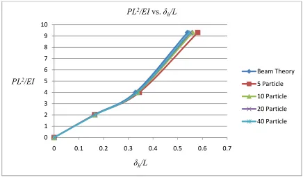
Figure 2.12. PL2/EI vs. δv/L ... 24

Figure 2.13. PL2/EI vs. δh/L ... 25

Figure 2.14. 3D Stretching Elements ... 27

Figure 2.15. Triangular Mesh with Emphasis on Two Elements Sharing Common Edge ... 28

Figure 2.16. 3D Triangular Mesh- Undeformed and Deformed Elements ... 29

Figure 2.17. Applied Uniform Pressure on Element 1-2-4 ... 37

Figure 2.18. Flexible Structure: Triangular Mesh ... 39

Figure 2.19. Simply Supported on all Four Sides, Center Point Load ... 40

Figure 2.20. δz/Lx vs. x: Particle Model Compared with First 11 Terms of Plate Theory (for y = 0.5) ... 42

Figure 2.21. δz/Lx vs. kb, Point Load, 4 Simply Supported Edges, Center Particle ... 43

Figure 2.22. Simply Supported on Two Edges with a Center Point Load ... 44

Figure 2.23. Simply Supported on Two Edges with a Line Load ... 46

Figure 2.24. Simply Supported on all Four Edges with a Center Point Load ... 47

Figure 2.25. Simply Supported on all Four Edges with a Line Load ... 49

Figure 3.1. Defining the Ultimate Goal of the Contact Algorithm ... 52

Figure 3.2. Possible Contact Situations ... 53

Figure 3.3. Plane ijk ... 54

Figure 3.4. Closest Projection of Point P onto the Plane ... 56

Figure 3.5. Before and After Configurations used to Define Contact ... 57

(11)

Figure 3.9. Current and Predicted Impactor and Structural Element Vertex

Positions ... 66

Figure 3.10. Velocity Update Applied at Contact Vertices ... 68

Figure 3.11. Front View of the Distance Check Method ... 70

Figure 3.12. Front-View of the Box Method ... 71

Figure 4.1. Cantilever Bending Test Apparatus ... 73

Figure 4.2. Overhang Length of the Fabric ... 74

Figure 4.3. Simply Supported Rectangular Plate Used for the Tuning Approach ... 79

Figure 4.4. Particle Mesh Used for Bending Stiffness Tuning ... 80

Figure 4.5. kb vs. P ... 82

Figure 5.1. Case 1 Initial Flexible Structure and Impactor Configuration ... 85

Figure 5.2. Forces and Velocity versus Time Plot ... 86

Figure 5.3. Single Impactor Triangle Animation Sequence ... 88

Figure 5.4. Time-History Plot for Structural Element Vertex 276 ... 89

Figure 5.5. Time-History Maximum Penetration ... 90

Figure 5.7. Multiple Impacts with Flexible Structure Animation Sequence ... 94

Figure 5.9. Single Impactor Triangle, Glancing Blow Animation Sequence ... 98

Figure 5.10. Case 4 Initial Flexible Structure and Sphere Configuration ... 100

Figure 5.11. Forces and Velocity versus Time Plot ... 101

Figure 5.12. Sphere Through Plate Slit Animation Sequence ... 103

Figure 5.13. Initial Configuration of Soldier and Full Hexagonal-shaped Tent ... 105

Figure 5.14. Pan View of Initial Soldier and Tent Configuration ... 106

Figure 5.15. Single Soldier Entering Full Hexagonal-Shaped Tent Animation Sequence... 108

Figure 5.16. Location of Vertex 1872 ... 110

Figure 5.17. Particle Model Comparison with LS-DYNA Vertex 1872 ... 111

Figure 5.18. Comparison Between Particle Model and LS-DYNA Animation Sequence... 112

Figure 5.19. Single Soldier Entering Full Tent with Pressure Animation Sequence .... 118

(12)

1 Introduction

1.1 Background and Objective of Research

(13)

Simulator to be updated to incorporate pre-programmed, mission-specific human activity and to link with existing urban airflow models that will provide external environmental conditions. Also, there is a need to add a particle model for fabric structural response to enable realistic simulations of flexible or semi-rigid entryways. The contribution of this research project stems from this need to add a particle model.

(14)

field near the door. Two-way coupling of the Room Simulator and particle code has not yet been completed but the capability to do so is available.

1.2 Literature

Review

The interest in physically-based models for cloth animation goes back over two decades. A physical model is one which provides physically realistic simulations based on the laws of physics. Research on these topics is very closely related to the textile and computer graphics industries. Early models were kinematic until Terzopoulos et al. (1987) began creating a physical model based on the theory of elasticity. The development of a physically-based model continued with Terzopoulos and Fleischer (1988), who saw the importance in using inelastically deformable models.

Particle models use particles arranged in triangular or quadrilateral elements to model a given fabric. Membrane stiffness can be modeled using interaction between a given particle and its nearest neighbors while bending stiffness can be modeled employing common edges between two elements. When dealing with large deformation drape response of fabrics, buckling is another important behavior which must be accounted for through bending stiffness. In addition to buckling behavior, collision detection is critical for accurate particle models and has been handled many different ways. This discussed in more detail below.

(15)

original material. Eischen et al. (1996) used finite-element modeling to simulate 3D motions related to the real fabric manufacturing process used in the textile and apparel industries. The issues they discussed are nonlinear material response, fabric contact with rigid surfaces, and adaptive arc-length control. Furthermore, Fontana et al. (2004) present a physical model which simulates multi-layered fabric for virtual prototyping applications. Their research follows from the woven material fabric and the use of a Kawabata bending test as described by Breen et al. (1994). Fontana et al. use a computer-aided design (CAD)-oriented system to make their contribution to the apparel manufacturing industry more useful.

(16)

Witkin (1998) were one of the first to successfully implement large time-steps in cloth simulation. Their contribution was to couple a new technique for constraining individual cloth particles with a modified conjugate gradient method to solve the linear system generated by the implicit integrator. Their simulation stably handles large time-steps.

Another way to speed up the computational time for collision detection is to incorporate a more efficient searching and detection scheme. Zhang and Yuen (2000) use a voxel-based collision detection method for clothed human animation. An assumption they use is cloth and human models are represented by triangular meshes. Then, they only treat edge-to-triangle collisions: an edge of a edge-to-triangle intersects another edge-to-triangle. A voxel is a uniform spatial subdivision of the object space. Collision triangles are limited to the voxels associated with that edge of the triangle. As a result, the number of potential collision regions is limited and potential collision regions can be located quickly.

(17)

Volino and Thalman (1994) was used. After collision is detected, they implement a correction on the particle acceleration rather than directly correcting the state of the system. In order to improve collision resolution in cloth simulations, Huh et al. (2001) introduce a collision detection scheme using swept-volumes which are volumes made up of two sets of positional entities at a face; one at time t and one at time t + Δt. Detected collisions are saved in a data structure known as, “zones of impact”. Then, to resolve collisions they use a cloth collision resolution method to simultaneously solve collisions while ensuring the conservation of momentum.

(18)

cloth after pinching based on a global intersection analysis of the cloth. They also present a method called flypapering, to handle pinches caused by cloth/solid collisions.

To improve drape simulation speed, Sul and Kang (2004) use a height and radial constraint to detect collisions. This includes cloth/cloth and cloth/human collisions. The fabric patterns were made into finite elements and given a local area number; only elements within a certain area can contact. The result is faster collision detection resulting in improved drape simulation speed.

More recently, Zink and Hardy (2007) have proposed a method of using geometry images in cloth simulation. Geometry images allow for the representation of a triangulated mesh as a regular 2D image file. Geometry images were introduced by Gu et al. (2002) to store surface geometry in a completely regular structure. Improvements to existing methods were achieved through the use of an implicit/explicit integration scheme by utilizing the regular structure of geometry images to improve performance. The demand for simulating real-time cloth motion is increasing and this method can provide this real-time simulation.

(19)

penetration. This method is very common and works well although violations of the penalty method are possible.

There has been an extensive amount of research done involving particle models, finite element analysis and collision detection/resolution for the textile and computer graphics industries. Free-falling cloth, the draping of cloth over solid objects (i.e. tables, chairs, blocks, balls, etc.) and modeling clothing on the human body are some of the most common examples. Other examples include flags waving and drapes blowing in the wind. One interesting case done by Huh et al. (2001) involves cloth draped over a solid ring; a ball is dropped on the cloth so both the ball and the cloth fall through the ring. Also, research done by O’Brien et al. (1997) introduces the combination of active and passive simulations for secondary motion. Some interesting examples examined through their simulations are: a gymnast on a trampoline, a bungee jumper, a gymnast vaulting on a mat, a girl swinging while wearing a skirt, and kites in the air. The primary contribution of the work is to examine three types of coupling: full, partial and one-way which they describe through the example of a basketball going through the net.

(20)

2 Particle Method Formulation

This chapter contains the development of the stretch and bend forces used in the particle method. In order to do so, these forces were first formulated in one-dimension and validated using beam theory. Then, these forces were formulated in three-dimensions and validated using plate theory. Additional forces which were assembled in the equations of motion include: gravitational forces, damping forces, external forces, and the effective force due to pressure.

2.1 One-Dimensional

Formulation

As a logical first step, a simple one-dimensional treatment of the particle method accounting for stretch, bend, damping, and external forces is introduced. Then, to validate the MATLAB computer code, results comparing the code to beam theory are presented.

2.1.1 One-Dimensional Stretch Formulation

(21)

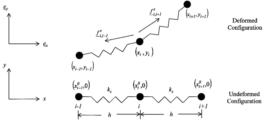
Figure 2.1. Stretching Elements

Figure 2.1 shows the undeformed and deformed configurations of particle i and its nearest neighbors. Unit vectors directed along the x and y coordinate directions are denoted ex and ey. The position vectors of the three particles under consideration are xi, xi-1, and xi+1.

y i x i

i x e y e

x   (2.1)

y 1 i x 1 i 1

i x e y e

x_  _  _ _(2.2)

y 1 i x 1 i 1

i x e y e

x_  _  _ (2.3)

The stretching forces shown acting on particle i due to particles i-1 and i+1 are the forces,

fi,i-1 and fi,i+1, respectively. The force on particle i due to particle j (j is either i-1 or i+1 in

Figure 2.1) was taken from Choi and Ko (2002) and given as

 

ij

(22)

i j

ij x x

x   _(2.5)

where |xij| is the magnitude of xij and h is the distance or natural length between particles i

and j in the undeformed configuration, defined as

0 ij

x

h  (2.6)

In equation 2.6, the superscript 0 refers to the particle coordinates in the undeformed configuration. Then, ks in equation 2.4 is replaced by k0/h and written as

 

ij ij ij

0 s

i _x

x h x h k

f   _(2.7)

The stretching stiffness coefficient (which is mesh size dependent) value k0/h was determined

by the following procedure:

(23)

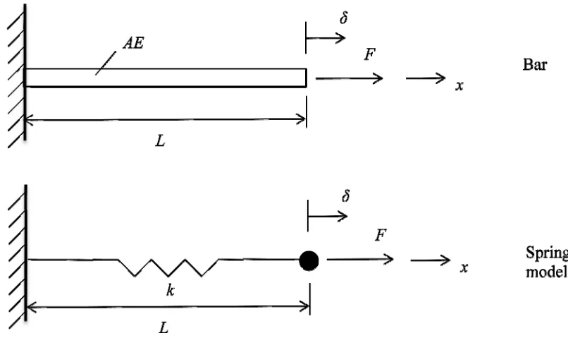
Figure 2.2 shows a single spring particle model of a classical bar element. The spring constant k = AE/L, where A is the cross-sectional area, E is the modulus of elasticity, and L is the length of the bar. The force-deflection response of the spring model (or the bar) is

 

L AE k

F   (2.8)

Figure 2.3 shows the case where multiple springs have been used to model the same bar. The spring constant for each of the springs is ks.

Figure 2.3. Multiple Spring Model of a Bar

Figure 2.3 shows the spring model with three springs (as an example) where ks is the

effective spring constant (equivalent to the particle spring). It is then desired to have equal deflection δ for the single and multiple spring models. For a particle model with n number of springs, the force-deflection response is



n k

F_ s _(2.9)

(24)

h k n L

kL L L nk nk

k 0

s    

/ (2.11)

Note again that h is the particle spacing.

Then, boundary conditions require special considerations.

Figure 2.4. Fixed Displacement Boundary Condition for Particle 1

Figure 2.4 shows a fixed displacement boundary condition when the particle being examined is particle 1. When particle 1 is in question, there is a force on particle 1 due to particle 2,

s 12

f . An auxiliary particle (fixed position, no position update during simulation) must be placed at position x = y = 0 during calculation of the force ( s

10

f ) on particle 1 due to the fixed displacement boundary condition.

(25)

Figure 2.5 shows a free edge boundary condition when the particle being examined is particle

n, the last particle. In this case, since there are no particles following particle n, the only force accumulated on particle n is from particle n-1, s

1 n n

f _

, .

2.1.2 One-Dimensional Bend Formulation

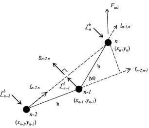
In order for a particle mesh to resist bending deformation, the curvature of the particle mesh must be considered. Curvature can be related to the incremental angle change between neighboring particles, as shown in Figure 2.6. The one-dimensional model was developed to include bend forces that resist bending deformation. The bending model has the ability to handle large deflections, as well as small deflections, with small relative rotation. When talking about small relative rotation, this refers to the angle Δφ in Figure 2.6. In order to calculate Δφ, the unit vectors ti-1,i, ti,i+1 and ti-1,i+1 must be calculated in terms of the particle

(26)

Figure 2.6. Bending Stiffness Element

Figure 2.6 shows a schematic of the bend forces applied to particles i-1, i, and i+1 that resist the bending deformation. In order to find the forces, b

1 i

f _ ,fb_i , and fb_i_₁, the following unit

vectors ti-1,i, ti,i+1 and ti-1, i+1 are defined as:

(27)



 



2 1 2

1 ,

1  

 i  i  i  i  i

i x x y y

t (2.15)



 



2

1 2 1 1

,i i i i i

i x x y y

t        (2.16)



 



2

1 1 2 1 1 1 ,

1     

 i  i  i  i  i

i x x y y

t (2.17)

The vector ni-1,i+1 is normal to the ti-1,i+1 vector and is computed using a cross product

y x 1 i 1 i x y 1 i 1 i 1 i 1 i z 1 i 1

i e t t e t e

n_ _,_   _ _,_  __,_  _ _,_ _(2.18)

where ez = ex × ey.

Referring to Figure 2.6, Δφ is the angle between the vectors ti,i+1 and ti-1,i and is referred to as

the bend angle.



ti,i 1y



arcsin



ti 1,iy



arcsin _  _



 (2.19)

The curvature at particle i is then approximated using

h

i 

  (2.20)

Then, the bend forces are taken from Bigliani and Eischen (2000) given by

1 i 1 i i b b 1

i 2k _h n

f _    ,

 (2.21) 1 i 1 i i b b

i 4k _h n

f   ,

 (2.22) 1 i 1 i i b b 1

i 2k _h n

f _    ,



(28)

Similar to handling stretching, bending also requires special consideration at boundaries.

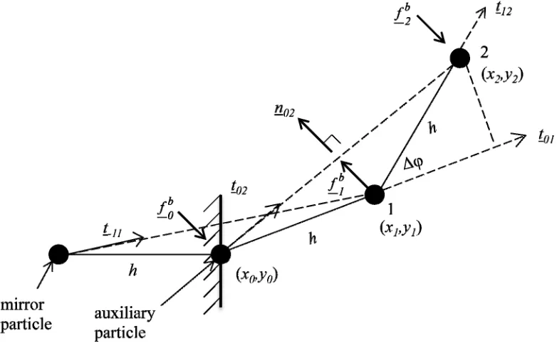
Figure 2.7. Fixed Displacement Boundary Condition for Particle 1

Figure 2.7 shows how a mirror particle and an auxiliary particle must be added to the model when the particle being examined is particle 1, and a fixed edge is present (zero deflection and slope). The reason for this is the bend forces assembled for particle 1 depend on κ0, κ1

and κ2. In order to find κ0, the equations given above must be used with the mirror particle,

auxiliary particle, and particle 1. When examining particle 2, this case differs from the general case because it depends on κ1. Therefore, the auxiliary particle needs to be used when

(29)

Figure 2.8. Free Edge Boundary Condition for Particle n

Figure 2.8 shows a particle at a free end with an applied external force. The curvature, κn at

the free end is set to zero. As a result, the only force assembled on particle n is due to the curvature at particle n-1, κn-1. Particle n-1 also does not accumulate the three forces fb_i_₁, fb_i ,

and b 1 i

f _ but simply fb_i_₁ and fb_i since κn = 0, fb_i_₁= fb_n = 0.

2.1.3 Damping Force

(30)

i d

i cv

f  (2.24)

where c is the damping coefficient and vi is the velocity vector at particle i.

2.1.4 One-Dimensional Equation of Motion

Once the stretch, bend, and damping forces have been accumulated for all particles, an equation of motion for the typical particle i can be written as

i ext i d i b i s

i f f f ma

f     (2.25)

where fext_i is the external force applied at particle i, m is the mass of particle i, and ai is the

acceleration vector of particle i. A similar equation of motion is written for each particle. In this work it has been assumed that the particle mass m was the same for each particle.

2.1.5 One-Dimensional Validation with Beam Theory

(31)

Figure 2.9 shows the parameters used in standard small deflection beam theory for the deflection of a cantilever beam with a tip load P. The equation for the deflection curve is given as,



L x



EI Px

y  3 

6 2

(2.26)

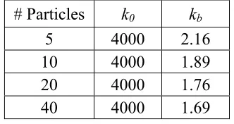
The tip deflection for beam theory was fixed at _max= 0.1 using P = 1, L = 1, EI = 3.333. The deflection curve for beam theory was plotted and used as the baseline for comparison in Figure 2.10. The stiffness coefficient values that were required to match the beam theory tip deflection are shown in Table 2.1.

Table 2.1. Particle Model Stiffness Coefficient Values

# Particles k0 kb

5 4000 2.16

10 4000 1.89

20 4000 1.76

40 4000 1.69

(32)

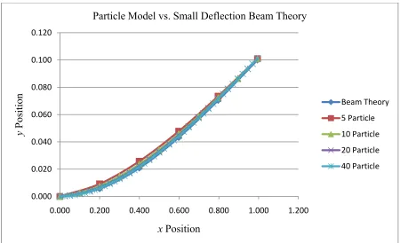
Figure 2.10. Bending Model vs. Small Deflection Beam Theory

Figure 2.10 shows the entire deflection curve for beam theory and the particle method for four different particle meshes. The deflection curve predicted by the particle model converged to the small deflection theory between the ends of the beam.

After finding the model agreed with standard small deflection beam theory, it was validated by large deflection beam theory as well.

0.000 0.020 0.040 0.060 0.080 0.100 0.120

0.000 0.200 0.400 0.600 0.800 1.000 1.200

y

Position

xPosition

Particle Model vs. Small Deflection Beam Theory

Beam Theory

5 Particle

10 Particle

20 Particle

(33)

Figure 2.11. Large Deflection Beam Theory Parameters

Figure 2.11 shows the parameters used in large deflection beam theory where δh is the

longitudinal tip deflection, δvis the transverse tip deflection, θb is the tip rotation, P is the

applied load, and L is the length of the beam. This is based on the formulation presented in Mechanics of Materials by Gere and Timoshenko (1997). For large deflection beam theory,

 

, )

( 2

k F k F EI

PL _ _ _(2.27)

where

2 sin

1 _b

k    (2.28)

and

       

2 1 sin 1

k

 (2.29)

(34)

 



 



0 ₁ 2_sin2 , t k dt k F _(2.31)

The dimensionless transverse tip deflection δv/L is

   









, 4

1 ₂ E k E k

PL EI L

v _ _ _ _(2.32)

where E(k) is the complete elliptic integral of the 2nd kind

 

 2  0 2 2_sin 1  tdt k k E (2.33)

and E(k,φ) is the incomplete elliptic integral of the 2nd_kind

 

  

0

2 2_sin 1

, k tdt

k

E (2.34)

The dimensionless longitudinal tip deflection δh/L is

2 sin 2 1 PL EI L b h     (2.35)

As a result, given the values θb and PL2/EI, the deflections δv/L and δh/L can be obtained

from large deflection beam theory. If PL2/EI is known, the corresponding load which must be applied to the particle model can be determined since L and EI are also known. Then, after calculating the load which must be applied, it was possible to obtain deflection values, δv/L and δh/L from the particle model. The stiffness values used for the particle model with

(35)

The comparison results for δv/L and δh/L between large deflection beam theory and the 40

particle model are shown in Table 2.2. The data used for the comparison was the same data used for small deflection theory validation.

Table 2.2. Comparison Results: Large Deflection Theory vs. 40 Particle Model

Large Deflection Theory 40 Particle Model

θb δh δv δx % Error δv % Error

0.785 0.16213 0.49551 0.166 2.6% 0.505 1.9% 1.12 0.32912 0.67011 0.336 2.1% 0.682 1.8% 1.41 0.53935 0.80286 0.548 1.7% 0.818 1.9%

The results in Table 2.2 show the percent error values between the deflection values for large deflection theory and the 40 particle model are all less than 2.6 %. This shows that using the

k0and kb values tuned for small deflection theory worked for large deflection theory as well.

0 1 2 3 4 5 6 7 8 9 10

0 0.2 0.4 0.6 0.8 1

PL2_/EI

PL2_/EI_vs._δ v/L

Beam Theory

5 Particle

10 Particle

20 Particle

(36)

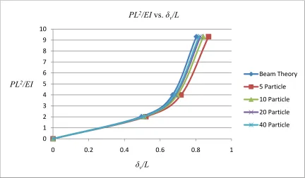
Figure 2.12 displays PL2/EI versus δv/L for the large deflection beam theory and the four

particle model meshes. As the number of particles increased, the particle model converged to the beam theory curve. This is representative of the deflection values presented in Table 2.2.

Figure 2.13. PL2_/_EI_vs._δ

h/L

Figure 2.13 shows the results of PL2/EI versus δh/L for large deflection beam theory and the

four particle model meshes. Again, as the number of particles increased, the particle model results converged to the beam theory results. From the results in Figure 2.10, Table 2.2 and Figures 2.12 and 2.13, the particle model has been shown to agree with small deflection theory as well as large deflection theory.

0 1 2 3 4 5 6 7 8 9 10

0 0.1 0.2 0.3 0.4 0.5 0.6 0.7

PL2_/EI

δh/L PL2_/EI_vs._δ

h/L

Beam Theory

5 Particle

10 Particle

20 Particle

(37)

2.2 Three-Dimensional

Formulation

In this section, the forces used in the three-dimensional MATLAB computer code are formulated. Additional forces added to the model which were not included in the one-dimensional formulation are: gravitational forces and the effective force due to pressure. In the three-dimensional formulation, a triangular mesh data structure was used by the particle model. The motivation for this mesh structure was the desire to read STL files as input and write STL files as output. STL files use a triangular data structure where the normal to the element and the coordinates of each triangular element vertex are provided. Each vertex for a given triangular element represents a particle on the flexible structure mesh. Using a triangular mesh data structure lends itself well to working with STL files.

2.2.1 Three-Dimensional Stretch Formulation

(38)

Figure 2.14. 3D Stretching Elements

Figure 2.14 shows the forces on particle i from a general number (n) of neighbor particles. The force f_is is then the force on particle i due to particle j and is given by





 



n

1

j _ij

ij ij

0 s

i _x

x h x h k

f _(2.36)

where k0 = ksh is the mesh size dependent stretch stiffness coefficient and z

i y i x i

i x e y e z e

x    _(2.37)

z j y j x j

j x e y e z e

x    _(2.38)

(39)

i j

ij x x

x   _(2.39)

And again |xij| is the magnitude of xij and h is the spacing between particles i and j in the

initial undeformed configuration.

0 ij

x

h (2.40)

2.2.2 Three-Dimensional Bend Formulation

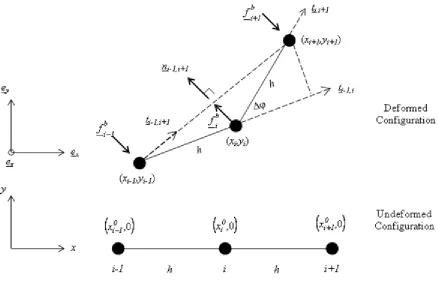
The three-dimensional bend formulation is a direct extension of the one-dimensional case. Figure 2.15 shows an arbitrary triangular mesh with a zoomed-in view on two typical elements which share a common edge.

Figure 2.15. Triangular Mesh with Emphasis on Two Elements Sharing Common Edge

(40)

to compare the angle change between element 1-2-4 and element 2-3-4. The notation 1-2-4 and 2-3-4 indicates the vertex node numbers of the two elements under consideration. This angle change is termed the bend angle, Δφ. Figure 2.16 shows element 1-2-4 and element 2-3-4 in the undeformed and deformed configurations in which bending occurs along the common edge 2-4. The vectors and unit normal vectors needed to find Δφ are also shown in Figure 2.16.

(41)

In order to compute the required normal vectors, several auxiliary vectors are needed. The unit vector directed along the edge between vertices 1 and 2 is

z z 12 y y 12 x x 12

12 t e t e t e

t    _(2.41)

where the components of t12 are





12 1 2 12 t x x

t _x   _(2.42)





12 1 2 12 t y y

t _y   _(2.43)





12 1 2 12 t z z

t _z   _(2.44)

and



 







2

1 2 1 2 2 1 2 2 1 2

12 x x y y z z

t       (2.45)

The unit vector directed along the edge between vertices 1 and 4 is

z z 14 y y 14 x x 14

14 t e t e t e

t    (2.46)





14 1 4 x 14 t x x

t   _(2.47)





14 1 4 y 14 t y y

t   _(2.48)

(42)



 







2

1 2 1 4 2 1 4 2 1 4

14 x x y y z z

t       (2.50)

Then, the unit normal vector to element 1-2-4 is computed using a cross product according to

z z 124 y y 124 x x 124 14 12 14 12

124 n e n e n e

t t

n   

 

 _(2.51)

where



12y 14z 12z 14y



x



12z 14x 12x 14z



y



12x 14y 12y 14x



_z 14

12 t t t t t e t t t t e t t t t e

t        _(2.52)

and

















2

1 2 x 14 y 12 y 14 x 12 2 z 14 x 12 x 14 z 12 2 y 14 z 12 z 14 y 12 14

12 t t t t t t t t t t t t t

t        (2.53)

Finally, the components of n124 are





14 12 y 14 z 12 z 14 y 12 x 124 t t t t t t n    (2.54)





14 12 z 14 x 12 x 14 z 12 y 124 t t t t t t n    _(2.55)





14 12 x 14 y 12 y 14 x 12 z 124 t t t t t t n    (2.56)

A similar calculation is required to construct the unit normal vector for element 2-3-4. The vector directed along the edge between vertices 2 and 3 is

z z 23 y y 23 x x 23

23 t e t e t e

t    _(2.57)

(43)





23 2 3 x 23 t x x

t   _(2.58)





23 2 3 y 23 t y y

t   _(2.59)





23 2 3 z 23 t z z

t   _(2.60)

where



 







2

1 2 2 3 2 2 3 2 2 3

23 x x y y z z

t       (2.61)

The unit vector directed along the edge between vertices 2 and 4 is

z z 24 y y 24 x x 24

24 t e t e t e

t    _(2.62)





24 2 4 x 24 t x x

t   _(2.63)





24 2 4 y 24 t y y

t   _(2.64)





24 2 4 z 24 t z z

t   _(2.65)

where



 







2

1 2 2 4 2 2 4 2 2 4

24 x x y y z z

(44)

z z 234 y y 234 x x 234 24 23 24 23

234 _t _t n e n e n e

t t

n   

 

 _(2.67)

where



23y 24z 23z 24y



x



23z 24x 23x 24z



y



23x 24y 23y 24x



_z 24

23 t t t t t e t t t t e t t t t e

t        _(2.68)

and

















2

1 2 x 24 y 23 y 24 x 23 2 z 24 x 23 x 24 z 23 2 y 24 z 23 z 24 y 23 24

23 t t t t t t t t t t t t t

t        (2.69)

Finally, the components of n234 are





24 23 y 24 z 23 z 24 y 23 x 234 t t t t t t n    _(2.70)





24 23 z 24 x 23 x 24 z 23 y 234

t

n







_(2.71)





24 23 x 24 y 23 y 24 x 23 z 234 t t t t t t n    _(2.72)

The vector bisecting the angle between n124 and n234 is simply the average of n124 and n234

z z 234 z 124 y y 234 y 124 x x 234 x 124

avg ₂ e

n n e 2 n n e 2 n n

n       (2.73)

(45)

z z 24 y y 24 x x 24

24 n e n e n e

n n

n    

avg avg

(2.75)

where the components of n24 are

avg x 234 x 124 x 24 n 2 n n n         (2.76) avg y 234 y 124 y 24 n 2 n n n         (2.77) avg z 234 z 124 z 24 n 2 n n n         (2.78)

Referring to Figure 2.16, the angle between the unit normal vectors n124 and n234 (bend angle)

is



124 234



1 234

12 n n n

t

sign  

 

_ ₍ ₎_cos

) (

cos )

(t₁₂ n₂₃₄ 1 n₁₂₄_xn₂₃₄_x n₁₂₄_yn₂₃₄_y n₁₂₄_zn₂₃₄_z

sign   

 

_ 

(2.79)

(46)

It has been assumed that negligible stretch exists and that the distance between vertices 1 and 3 changes very little during deformation. So, the curvature defined by the relative rotation between the elements is,

0 13

h



 _(2.81)

Finally, the bend forces are constructed following the one-dimensional treatment, with an adjustment to account for the fact that they are directed along n24

24 0 13 b b

1 2k _h n

f   _(2.82)

24 0 13 b b

2 2k _h n

f   _(2.83)

24 0 13 b b

3 2k _h n

f   _(2.84)

24 0 13 b b

4 2k _h n

f   _(2.85)

2.2.3 Boundary Conditions

(47)

2.2.4 Initially Curved Surfaces

For a flexible structure which begins as a curved surface or its elements meet at a curved junction, an initial curvature was computed. The initial curvature for each bend element was stored. Then, the bend forces depend on the difference between the current and the initial curvature.

2.2.5 Gravitational Forces

In order to produce realistic results, a gravitational force was incorporated in the formulation. The gravitational force is given simply as,

z z i y y i x x i z gz y gy x gx g

i f e f e f e mg e mg e m g e

f       (2.86)

where mi is the particle mass and either gx, gy, or gz is equal to the gravitational acceleration

constant g, depending on the direction in which gravity acts.

2.2.6 Effective Force due to Pressure

(48)

Figure 2.17. Applied Uniform Pressure on Element 1-2-4

As the unit normal vector and the pressure are oriented in Figure 2.17, the effective forces acting on the element vertices are calculated according to

124 p

i ₃ n

pA

f  (2.87)

where A is the element area. If the pressure and unit normal vectors are oriented in opposite directions, a negative sign would be introduced in equation 2.87.

2.2.7 Damping Force

As with the one-dimensional formulation, a velocity dependent force was included in the three-dimensional formulation to enable damping of structural motions, if desired. An absolute damping approach was used and the damping force was calculated according to

i d

i cv

f  (2.88)

(49)

2.2.8 Equations of Motion

The equation of motion for particle i can be written as

i i ext i d i p i g i b i s

i f f f f f m a

f       (2.89)

where mi is the mass of particle i and ai is the acceleration vector for particle i.

MATLAB has been used to implement the particle element formulation algorithm. Appendix A contains the MATLAB particle code that accumulates the equations of motion for all of the particles. An explicit fourth-order Runge-Kutta method (Abramowitz & Stegun, 1972) was employed to solve the equations of motion. Refer to Appendix B for the fourth-order Runge-Kutta MATLAB code.

2.2.9 Three-Dimensional Validation with Plate Theory

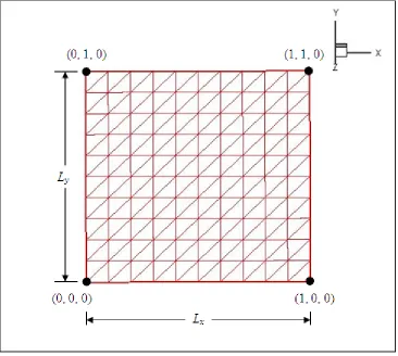
To validate the particle model, results obtained from the particle model were compared with the results from classical plate theory (Timoshenko & Woinowsky-Krieger, 1959). To obtain results, an initially flat, square flexible structure with dimensions Lx = Ly = 1 (arbitrary units)

(50)

Figure 2.18. Flexible Structure: Triangular Mesh

(51)

Figure 2.19. Simply Supported on all Four Sides, Center Point Load

The formula for the deflection of such a square plate from the classical theory is

  _                                        terms 1 m terms 1 n _y y x 2 2 y 2 2 x 2 y x y x 4 z L y L n L x m L n L m L n L m D L L P

4 # # ( )

sin sin sin sin       _(2.90)

where D is the bending/flexural rigidity of the plate, ζ is the x-location of the load point, η is the y-location of the load point, while x and y are the coordinates of the point in question. For the maximum deflection at the center, equation 2.90 reduces to





      terms terms 2 2 2 4 2 x z 1 D PL

4 # #



(52)

the maximum particle model deflection to 0.1 ≤ 0.001 for the given applied load P. The value of D was adjusted in computation of the theoretical deflection so that the center deflection predicted by plate theory matched the particle model result (both giving δz =

0.1004). The required value for D was 0.11509.

Table 2.3 shows the results of the particle model deflection compared with the theoretical results.

Table 2.3: Square Plate, Deflection Results, Comparing Particle Model with Plate Theory

Particle Model Plate Theory

x y δz δz % Error

0 0.5 0.0000 0.0000 0.0% 0.1 0.5 0.0232 0.0221 4.8% 0.2 0.5 0.0474 0.0540 12.2% 0.3 0.5 0.0704 0.0796 11.5% 0.4 0.5 0.0902 0.0952 5.3% 0.5 0.5 0.1004 0.1004 0.0% 0.6 0.5 0.0902 0.0952 5.3% 0.7 0.5 0.0704 0.0796 11.5% 0.8 0.5 0.0474 0.0540 12.2% 0.9 0.5 0.0232 0.0221 4.8%

1 0.5 0.0000 0.0000 0.0%

(53)

assumption with plate theory is it is based solely on bending stiffness; membrane (stretching) stiffness is neglected. When attempting to use the particle model with k0 = 0, the model did

not produce favorable results. Therefore, stretching stiffness was included in the model which may provide an explanation for the discrepancies between plate theory and the particle model. Figure 2.20 shows a graphical representation of the comparison of the deflection curves shown in Table 2.3.

Figure 2.20. δz/Lx vs. x: Particle Model Compared with First 11 Terms of Plate Theory

(for y = 0.5)

Figure 2.20 shows the particle model curve matches the plate theory curve between the edges very closely. The points on the curves which do not match exactly are highlighted by the

0 0.02 0.04 0.06 0.08 0.1 0.12

0 0.2 0.4 0.6 0.8 1 1.2

δ_z/L_x

x

δ_z/L_xvs. x

Plate Theory 11 Terms

(54)

Next, to investigate the effect of the bending stiffness coefficient on the deformation of the structure, deflection curves generated by the particle model were created as the value of kb

was varied for several values of k0. The flexible structure shown in Figure 2.18 was used to

produce the results for the load case and boundary conditions shown in Figure 2.19. Figure 2.21 shows δz/Lx vs. kb for the k0 values 1, 5, 10 and 20. The dimensionless deflection δz/Lx

was computed at the center particle.

Figure 2.21. δz/Lx vs. kb, Point Load, 4 Simply Supported Edges, Center Particle

Figure 2.21 shows the relationship between changing the k0 and kb values. When kb = 0, the

deflection decreases as k0 increases, as expected. Then, for a fixed value of k0, as kb

increases, the deflection converges to a fixed value (δz/Lx = 0.0045). Thus for very high

bending stiffness, the deflection was controlled by the stretching springs.

Then, to qualitatively check that the particle model was deforming as expected, contour plots

‐0.1 0 0.1 0.2 0.3 0.4 0.5 0.6 0.7

0 0.2 0.4 0.6 0.8

δz/Lx

k_b

δ_z/L_xvs. k_b: Point Load, 4 Simply Supported Edges, Center Particle

k0=1

k0=5

k0=10

(55)

conditions along with the contour plot of the final deformed mesh for the given load-case. The parameters used were: P = 1, Lx = Ly = 1.

(56)

direction with two simply supported edges, Figure 2.22 shows the contour plot of the final deformed shape of the mesh. The largest deflection (shown in red) occurred at the point of the applied load, as expected. The deformation of the mesh was symmetric, with the smallest deflection occurring at the two simply supported edges (shown in blue).

In the next case, the particle mesh was simply supported on two edges with a line load along

(57)

Figure 2.23. Simply Supported on Two Edges with a Line Load

(58)

Then, the next load-case was used to validate the particle model with plate theory. The mesh was simply supported on all four edges with a center point load applied in the positive z -direction. Figure 2.24 shows the loading and boundary conditions along with the final

contour plot of the deformed mesh for this case. The parameters used were: P = 1,

(59)

As expected, the largest deflection occurred at the point of the applied load and the deformation of the mesh was symmetric. The smallest deflection occurred at all four simply supported edges.

(60)

Figure 2.25. Simply Supported on all Four Edges with a Line Load

(61)

(62)

3 Contact

Formulation

One of the project goals was to account for the interaction between a rigid impactor, modeled as a moving surface meshed with triangular elements, with a flexible structure, also modeled with a triangular mesh of particles. The positions of the impactor vertices are tracked to detect whether they have crossed any elements on the flexible structure. The flexible structure was modeled with the particle method formulation discussed in the previous chapter. The basic contact detection scheme must determine whether the impactor vertices have pierced structural elements, and if so, appropriate action must be taken.

Contact is often times a very difficult, yet very important issue. When speaking of contact, there are generally two steps to every contact algorithm, contact detection and contact correction. The algorithm described in this chapter uses a point-to-plane contact detection scheme with an update made to the velocity of the element vertices when contact has been detected.

3.1 Contact

Detection

(63)

element was based on the point-to-plane method. Figure 3.1 shows the ultimate goal of implementing the contact algorithm: to handle the contact sequence of a human (modeled as a surface mesh of impactor vertices) and a tent door (modeled as a surface mesh of structural elements).

Figure 3.1. Defining the Ultimate Goal of the Contact Algorithm

This complex problem can be simplified by discussing a single impactor vertex, P and a single structural element i-j-k. Figure 3.2 introduces a schematic of the four possible contact situations for a given impactor vertex where element i-j-k is viewed on edge.

Each vertex which made up the human model was treated as an impactor The flexible structure is made up

(64)

Figure 3.2. Possible Contact Situations

(65)

possible contact situations which had to be accounted for when developing the contact algorithm.

Figure 3.3 shows vertices i, j, and k of a typical structural element. By definition these three vertices lie in a plane, shown in grey in the figure.

Figure 3.3. Plane ijk

Plane ijk is the plane defined by element i-j-k in the xyz-coordinate system. The position vectors of points i, j, and k are xi, xj, and xk, respectively where

e z e y e x

(66)

z k y k x k

k x e y e z e

x    (3.3)

The position vector of impactor vertex P is P where

z z y y x

xe P e P e

P

P   _(3.4)

Then, v1 is a vector which points from vertex i to j, v2 is a vector which points from vertex i to k, and v3 is a vector which points from vertex j to k, i.e.

z i j y i j x i j i j

1 x x x x e y y e z z e

v   (  ) (  ) (  ) _(3.5)

z i k y i k x i k i k

v   (  ) (  ) (  ) _(3.6)

z j k y j k x j k j k

v   (  ) (  ) (  ) _(3.7)

The unit normal to element i-j-k, pnorm, is found by taking the cross product of v1 and v2. Note that the unit normal pnorm discussed here in the contact development chapter is equivalent to

n124or n234developed in the three-dimensional bend formulation (Section 2.2.2).

2 1 2 1 z normz y normy x normx

norm _v _v

v v e p e p e p p       2 1 z x 2 y 1 y 2 x 1 y z 2 x 1 x 2 z 1 x y 2 z 1 z 2 y 1

norm _v _v

e v v v v e v v v v e v v v v p       ( ) ( ) ( ) (3.8)

(67)

Figure 3.4. Closest Projection of Point P onto the Plane

The vector viP which points from vertex i to point P is calculated according to

z i z y i y x i x i

iP P x P x e P y e P z e

v   (  ) (  ) (  ) _(3.9)

Then, the vector which points from Q to P along the normal direction pnorm is

norm iP norm z

QPz y

QPy x

QPx

QP v e v e v e p v p

v    (  ) (3.10)

The position vector of point Q can be obtained from QP

v P

Q  _(3.11)

The point Q does not necessarily lie within element i-j-k, only in the plane defined by element i-j-k.

(68)

Figure 3.5. Before and After Configurations used to Define Contact

(69)

contact occurs. It is necessary to determine which structural element, if any, contains the projection Q of a given impactor vertex. Therefore, determining whether or not point Q lies within element i-j-k is the next issue.

In order to do so, the distance from each vertex in element i-j-k to point Q is calculated. z i z y i y x i x

i Q x e Q y e Q z e

x Q

iQ  (  ) (  ) (  ) _(3.12)

and z j z y j y x j x

j Q x e Q y e Q z e

x Q

jQ  (  ) (  ) (  ) _(3.13)

and z k z y k y x k x

k Q x e Q y e Q z e

x Q

kQ  (  ) (  ) (  ) _(3.14)

Figure 3.6 shows the case when point Q is contained inside element i-j-k with vectors iQ, jQ, and kQ defined along with the subdivided areas A1, A2, and A3.

(70)

z x 2 y 1 y 2 x 1 y z 2 x 1 x 2 z 1 x y 2 z 1 z 2 y 1 2

1 ₂ v v v v e v v v v e v v v v e

1 v v 2 1

A   (  ) (  ) (  ) (3.15)

The three sub-areas defined by point Q and vertices i, j, k are

z x y 1 y x 1 y z x 1 x z 1 x y z 1 z y 1 1

1 ₂1 v iQ 1₂ v iQ v iQ e v iQ v iQ e v iQ v iQ e

A    (  ) (  ) (  ) _(3.16)

and z x 2 y y 2 x y z 2 x x 2 z x y 2 z z 2 y 2

2 ₂1 iQ v 1₂ iQ v iQ v e iQ v iQ v e iQ v iQ v e

A    (  ) (  ) (  ) _(3.17)

and z x y 3 y x 3 y z x 3 x z 3 x y z 3 z y 3 3

3 ₂ v jQ v jQ e v jQ v jQ e v jQ v jQ e

1 jQ v 2 1

A    (  ) (  ) (  ) _(3.18)

When point Q lies within element i-j-k, the total area A must be the same as the sum of the sub-areas, i.e.

3 2

1 A A

A

A   (3.19)

Flexible Structure Impact Modeling With a Particle Method.

DEDICATION

BIOGRAPHY

ACKNOWLEDGMENTS

TABLE OF CONTENTS

LIST OF TABLES

LIST OF FIGURES

1 Introduction

1.1 Background and Objective of Research

1.2 Literature

Review

2

Particle Method Formulation

2.1 One-Dimensional

Formulation

 

 



 





 





 















 

 

   





 

 

2.2 Three-Dimensional

Formulation



















 

 

















 

 



































