Live Axis Turning

(1)

ABSTRACT

Buescher, Nathan. Live-Axis Turning. (Under the direction of Thomas A. Dow)

(2)

LIVE-AXIS TURNING

NATHAN P. BUESCHER

A thesis submitted to the Graduate Faculty of North Carolina State University

In partial fulfillment of the Requirements for the Degree of

Master of Science

MECHANICAL ENGINEERING NORTH CAROLINA STATE UNIVERSITY

Raleigh, NC 2005

APPROVED BY:

____Dr. Ronald O. Scattergood___ ____Dr. Jeffrey W. Eischen____

(3)

BIOGRAPHY

(4)

ACKNOWLEDGMENTS

I would to thank everyone who helped, supported and guided me during my stay at NC State University. My time at the Precision Engineering Center gave me invaluable hands-on experience in so many areas and helped bridge the gap between the academic world and the real world for me. To the following people I am especially thankful.

• Dr. Thomas Dow, my advisor, for continually challenging me, teaching me how to think critically to solve problems and always asking more questions than I could answer.

• Alex Sohn, for being patient and putting in a lot of time with me on this project. Your practical nature and machining experience really taught me a lot.

• Ken Garrard, for much assistance with all computer-related issues and plenty of other concepts I was struggling to grasp, especially on the UMAC controller.

• Dr. Jeffrey Eischen and Dr. Ronald Scattergood, my committee members.

• Brett and Kara, for struggling through many classes and countless long nights at the PEC with me.

• All the other students at the PEC – Karl, Wittoon, Simon, Dave, Tim, Yanbo, Nadim, Lucas and Rob – for your help and for providing some good laughs.

• Laura Masters, for holding the place together during her time there.

• Stacey, for your love, support and especially patience during a seemingly endless journey.

• My brother William, for always providing laughter and good conversation.

(5)

LIST OF FIGURES

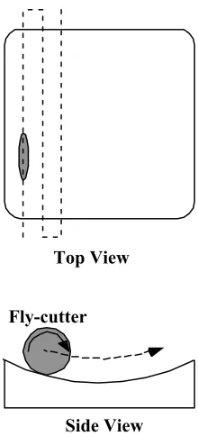
Figure 1-1. Raster scan diamond fly-cutting... 3

Figure 1-2. Diamond Turning Machine (DTM) with tool servo (Z') used to create NRS surfaces. The height of the surface is a function of the location on the face (x,y) or in polar coordinates, r and q... 4

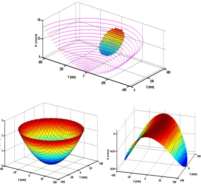
Figure 1-3. Decomposition of off-axis conic mirror surface (top) into symmetric (bottom left) and non-symmetric (bottom right) components for on-axis fabrication (different Z axis magnitudes should be noted)... 6

Figure 2-1. Front (left) and side views of general LAT design. ... 8

Figure 2-2. (a) A composite aluminum beam. (b) A closer look at the cell structure of the honeycomb [12]. ... 9

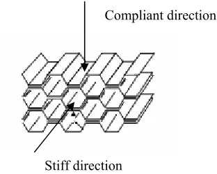
Figure 2-3. The orthotropic nature of the honeycomb core ... 13

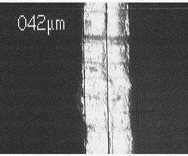
Figure 2-4. Aluminum facing skin, seen at 50X by the Zeiss ICM 405 microscope – approximately 1 mm (0.04 in.) thick. ... 14

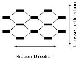
Figure 2-5. Ribbon and Transverse directions in the honeycomb cell structure. ... 15

Figure 2-6. Top view of honeycomb core at 200X on the Zeiss ICM 405 microscope. The bright section is two strips of aluminum joined at the faces, so the measured width (the thickness of one strip) is only one-half of the total width. ... 17

Figure 2-7. Instron testing machine. ... 18

Figure 2-8. An aluminum specimen in a four-point bending test ... 19

Figure 2-9. Load vs. Displacement for aluminum honeycomb specimen. ... 20

Figure 2-10. The elastic region of the honeycomb Load vs. Displacement plot (labeled in Figure 2-9). ... 20

Figure 2-11. Setup for frequency test. ... 21

Figure 2-12. Frequency response of aluminum honeycomb sample free-free test. Resonance occurs at 2.48 KHz. ... 22

Figure 2-13. Simulated four-point bending test on a beam of aluminum honeycomb modeled as two thin sheets of aluminum bonded to a honeycomb core. The load shown is 200 lb., and it corresponds to a deflection of 0.0078 in... 24

Figure 2-14. Load vs. Deflection plot for aluminum honeycomb of fixed geometry. Theoretical refers to the analytical solution, Experimental is from the Instron machine, and Model is the FEA results. ... 24

Figure 2-15. Free-free vibration of an aluminum honeycomb beam. This first free-body mode occurs at 2800 Hz... 25

Figure 2-16. The underside of an aluminum facing skin (with some honeycomb attached). The uneven distribution of the glue may have yielded a slightly lower natural frequency than a perfectly bonded specimen... 26

Figure 2-17. (Left) Simplified box design (darker, outer shell is aluminum; lighter parts are honeycomb). Cutout is needed so motor may be embedded. (Right) Box design shown with housing. The rectangle in the middle represents the slide shown on the left. ... 27

Figure 2-18. Simplified V-shape design (left) and V-shape slide with housing (right). . 28

Figure 2-19. Simplified view of the triangle design (left) and the housing for this design (right). ... 29

(8)

Figure 2-21. Vertical bending (left) and horizontal twisting modes of the

slide-bracket-coil assembly... 33

Figure 2-22. Rigid body modes of vibration due to the bearing... 34

Figure 2-23. Graphical comparison of structural and bearing natural frequencies... 35

Figure 2-24. Setup for the slide bending test. Force was applied at the vertex of the triangle, and the deflection was measured below. ... 37

Figure 2-25. Force vs. Deflection plot for the slide bending test. The elastic region is located inside the circle... 38

Figure 2-26. First (left) and second (right) predicted modes of vibration for the triangle slide. The first mode (twisting) occurs at 3950 Hz and the second (bending) at 5110 Hz (results from COSMOS FEA analysis). ... 39

Figure 2-27. Setup for the slide frequency analysis (left). An accelerometer is seen attached to the far right corner of the slide. The accelerometer amplifier is shown on the right. ... 40

Figure 2-28. Magnitude results from slide frequency test. When the slide was struck in the middle, a spike around 3550 Hz occurred (top plot). When struck at the corner, the dominant frequency was around 4660 Hz (bottom)... 41

Figure 2-29. Layout of the slide grid used in the frequency analysis... 42

Figure 2-30. Embedded motor coil design (left) and rear-attached motor coil design. ... 44

Figure 2-31. Cutaway view of a linear motor I-coil. The banded strands of copper wire can be seen. ... 45

Figure 2-32. Experimental setup for the motor coil bending test. ... 46

Figure 2-33. Original design of motor mount bracket. ... 47

Figure 2-34. The first mode of vibration of the system using the original bracket showed significant deflection in the bracket... 47

Figure 2-35. New bracket with thicker faceplate, horizontal gussets and lightweighting holes. ... 48

Figure 2-36. First bending mode with new bracket. Deformation now occurs in the slide and motor coil, indicating a sufficiently stiff bracket. ... 48

Figure 2-37. 3D drawing of the new rear faceplate of the slide. This view is from inside the slide looking toward the back. A relief (the large box) is provided for the magnet track, and the four small squares are used to hold the bracket screws... 50

Figure 2-38. Slide-bracket-motor assembly. The magnet track forms a channel around the bottom of the motor I-coil and extends into box-shaped relief area in the slide... 50

Figure 2-39. Final bracket design. ... 51

Figure 2-40. Photograph of LAT system. The slide and air bearing housing are shown. ... 51

Figure 2-41. Setup for air bearing stiffness measurements... 53

Figure 2-42. Renishaw RGH24B linear encoder with scale... 54

Figure 2-43. Tool holder mounted to the front of the triangular slide... 55

Figure 2-44. Flexure plate layout on the Nanoform. The box with the knob directly under the slide housing is the micro height adjuster. The notched plate directly above the micro height adjuster is the flexure plate. ... 56

Figure 2-45. Model of the flexure plate in its natural (left) and deflected (right) positions. ... 56

(9)

Figure 2-47. Final design drawings for the LAT system. Front and side view shown... 59

Figure 3-1. Main component layout of the LAT system. The arrows show the direction of command. ... 61

Figure 3-2. Block diagram of the entire system. The signal from the PC is compared to the current tool position, then sent to the UMAC. It is acted on by the controller and sent to the amplifier, which commutates the system based on the position feedback.62 Figure 3-3. Plot of motor temperature versus time. ... 65

Figure 3-4. Free-body diagram of the undamped LAT system ... 66

Figure 3-5. Open-loop block diagram of the undamped system... 67

Figure 3-6. Theoretical open-loop Bode plots of the undamped system. ... 68

Figure 3-7. Amplifier response to a closed-loop step command. ... 69

Figure 3-8. Experimental undamped transfer function compared with system model. ... 71

Figure 3-9. Free-body diagram of the damped system. ... 72

Figure 3-10. Root Locus plot for the undamped (a) and damped (b) systems. The addition of the damping force pushes the closed loop poles into the left-hand plane, indicating a stable system. ... 73

Figure 3-11. Step response of the damped and undamped system. While the damped system decays, the response of the undamped system maintains constant amplitude (marginally stable). ... 74

Figure 3-12. The damper for the LAT system. The rod shown slides through an O-ring sandwiched between the two brackets. ... 75

Figure 3-13. Diagram of rod (horizontal line) - O-ring (curved line) interface... 76

Figure 3-14. Viscous Damping Force vs. Edge Clearance. ... 77

Figure 3-15. Bode Plots for varying systems with varying damping forces. The "jagged" dotted line is the experimental data. ... 79

Figure 3-16. Open loop block diagram of the damped system. ... 79

Figure 4-1. Control layout for the LAT system. ... 81

Figure 4-2. Block diagram of UMAC PID control scheme... 84

Figure 4-3. Simulink model of the controller and motor system... 85

Figure 4-4. 156 µm step response of the undamped Simulink model. ... 87

Figure 4-5. Response of the Simulink damped model (b=10) to a 156 µm step. The rise time is roughly half that for the undamped system... 88

Figure 4-6. The response of the Simulink models to a 156 mm disturbance input over one servo cycle (442 µsec). The jump seen in the damped system is smaller than that of the undamped system... 89

Figure 4-7. Step response of the undamped system... 90

Figure 4-8. Undamped system response to 1 mm, 5 Hz sine wave. The top plot shows the command and actual motion, and the bottom plot shows the error between the two... 92

Figure 4-9. Phase error sine fit (top) and undamped system sine following error with phase lag removed... 93

Figure 4-10. Step response of damped system... 95

Figure 4-11. Damped system response to 1 mm, 5 Hz sine wave. The top plot shows the command and actual motion. The bottom plot shows the error between the two. ... 96

(10)

Figure 4-13. Setup for the disturbance rejection test. A string with a weight attached was tied to the motor bracket and hung over the pulley. The weight was dropped, and the system's motion was recorded... 98 Figure 4-14. Undamped (top) and damped (bottom) system response to external

disturbance, with the modeled/theoretical responses shown as dotted lines. A smaller peak value for the damped system shows it is more resistant to external forces... 99 Figure 5-1. LAT axis on the Nanoform 600. ... 100 Figure 5-2. Scanning White Light Interferometer (SWLI) image of the PMMA flat

machined at 500 rpm with a 1 mm/min feedrate. ... 102 Figure 5-3. Error motion (left) of the LAT axis (commanded minus actual position)

during machining at 500 rpm. The figure at right is the FFT of the error. ... 104 Figure 5-4. Tilted flat being measured by the coordinate measuring machine (CMM).

The non-tiled part was flat to less than 1 µm – beyond the resolution of the machine. ... 104 Figure 5-5. Top view of DTM during generation of the tilted flat ... 105 Figure 5-6. Tool tip contact with a flat surface (top) and a tilted surface (bottom). Tool

tip compensation is needed to eliminate the unwanted contact associated with a tilted surface... 106 Figure 5-7. The LAT position (top) and the associated tool radius compensation (bottom)

for a 1 mm radius tool and a 2mm peak-to-peak flat at 25 mm radius. The

compensation is always subtracted from the commanded position. ... 107 Figure 5-8. LAT axis error generated with the kinematics routine (position-based)... 109 Figure 5-9. LAT axis error generated by the time-based motion program. The 250 Hz.

frequency is no longer present. ... 110 Figure 5-10. Surface of the 2 mm PMMA tilted flat machined at 500 rpm with a 2.5

mm/min feedrate. The radial direction is approximately along the grooves. ... 111 Figure 5-11. PMMA tilted flat cutting data. The top plot shows the error during cutting.

The bottom plot shows the frequency content of the error. ... 113 Figure 5-12. The effect of the notch filter in the controller on the system performance.

... 115 Figure 5-13. 50 X 70 µm area of a flat machined without damping (Ra = 16 nm). The

spindle speed was 400 rpm and the federate was 0.84 mm/min... 116 Figure 5-14. LAT motion during position holding. The top plot (a.) shows the motion

reported by the LAT encoder. The bottom plot (b.) is Lion capacitance gauge data for the same experiment. ... 117 Figure 5-15. Cap gauge data collection setup... 118 Figure 5-16. Zygo Laser Interferometry image of the surface of the flat cut without

damping. The 12 mm surface is flat to less than ½ wave. The part was cut with a spindle speed of 400 rpm and a federate of 0.84 mm/min... 119 Figure 5-17. SWLI image of the flat cut with physical damping added to the system.

The spindle speed was 400 rpm and the federate was 0.84 mm/min... 120 Figure 5-18. Laser interferometry image of the flat cut with the damped LAT system.

The spindle speed was 400 rpm and the federate was 0.84 mm/min... 121 Figure 5-19. Surface of the undamped tilted flat. The part was cut at 300 rpm with a

(11)

Figure 5-20. FFT data of the LAT motion during cutting. A frequency of 150 Hz is

noticed, as was seen in the controller tuning. ... 123

Figure 5-21. Surface of the undamped aluminum tilted flat measured by the CMM. The top left plot is an isometric view of the surface. The top right plot shows the surface figure error (best fit plane residual), and the bottom plot is a side view of the error. ... 124

Figure 5-22. Talysurf trace from the low edge to the high edge of the undamped aluminum tilted flat with the slope taken out. The “hump and valley” shape confirms the CMM data in Figure 5-20. ... 125

Figure 5-23. Theoretical tilted flat with linearly varying phase lag throughout the cut. Theoretical tilted flat surface (top left), error (top right) and side view of the error (bottom). The shape is the same as that seen in the undamped aluminum flat... 126

Figure 5-24. Surface of the tilted flat cut with damping added to the system. The spindle speed was 300 rpm and the feedrate was 1.8 mm/min. ... 127

Figure 5-25. (Top) Surface of the damped aluminum tilted flat as measured by the CMM. (Top right) Error in the tilted flat and side view of error (bottom). The error has the same shape as that for the undamped tilted flat and is due to varying phase lag... 128

Figure 5-26. Talysurf trace from the low edge to the high edge of the undamped aluminum tilted flat with the slope taken out... 129

Figure A-0-1. The make-up of a honeycomb composite. In this application, the facing skin material is aluminum... 136

Figure A-0-2. Honeycomb beam deflection due to bending... 137

Figure A-0-3. Honeycomb beam deflection due to shear... 137

Figure A-0-4. The rotor and stator of a basic rotary motor. ... 142

Figure A-0-5. Pole-switching sequence for rotary motor rotation... 143

Figure A-0-6. Three phase power. The plot shows Current vs. Time. ... 143

Figure A-0-7. Linear motor 3D view (top). Motor schematic, viewed from above (bottom)... 144

(12)

LIST OF TABLES

Table 2-1. A comparison of weight and stiffness between two honeycomb beams and a

solid I-beam………...11

Table 2-2. List of values used to model honeycomb core………14

Table 2-3. Comparison between slide shapes………...30

Table 2-4. Comparison of V-shape and triangle slide designs. The triangle design was chosen because of its high stiffness and relative ease of assembly, shown by the fewer number of parts………32

Table 2-5. Comparison of the translational and rotational natural frequencies due to the bearing stiffness and the vertical and horizontal natural frequencies of structural vibration………...35

Table 2-6. Tool-tip moment stiffness for different slide lengths………..36

Table 2-7. Comparison of predicted and actual results for a slide frequency analysis….43 Table 2-8. Natural frequencies of the system for the two bracket designs………...49

Table 3-1. Mass of LAT system’s moving parts………...67

Table 4-1. Final gains used for the undamped LAT system………...94

Table 4-2. Final gains used for the damped LAT system………...97

Table A-1. Summary of beam coefficients……….138

(13)

1 Introduction

1.1 Background

The optical designer must address optical performance, space constraints, weight limitations, assembly/alignment issues and cost. The number and placement of optical elements depends on the application and the shape of each element. Based on experience and availability, the optical designer would typically choose spherical surfaces; however, aspheric (rotationally symmetric) elements are becoming common in many new designs. A more powerful alternative is to utilize anamorphic (non-rotationally symmetric) shapes such as off-axis conic or toroidal surfaces that can more efficiently collect and focus light while packaging the optical system into a smaller volume at lower cost. But the procurement of such optics is difficult, time consuming, and expensive. If the design consists of a series of spherical components, there is a large body of information available from a number of different manufacturers regarding fabrication capabilities. For Non-Rotationally Symmetric (NRS) surfaces however, fabrication capabilities are very limited. Hence, most designers tend to avoid anamorphic designs, even if such shapes could simplify the design, reduce the number of components and shorten the assembly time.

(14)

generate and polish. New machines and methods have been developed over the past decade to speed this process and the technical challenges associated with these processes have been addressed [1, 2, 30]. These techniques utilize a small grinding wheel that follows the desired aspheric contour as it is moved along the radius of the rotating part. This same concept has been applied to create NRS parts except that the rotation speed of the part is reduced drastically such that the slide axis can move as a function of radius and angle to produce the desired NRS contour. To polish such a surface, techniques such as small aperture polishing have been used. The disadvantage of these polishing processes is they are exceedingly slow and the form error can deteriorate if several cycles of measure and polish are employed.

(15)

Fly-cutter Top View

Side View

Figure 1-1. Raster scan diamond fly-cutting.

As a result, this process can require large amounts of time – sometimes days for a 100 mm square part. Long machining times will increase three things: the risk of anomalous events causing a defect, the drift in environmental conditions degrading the figure and finish, and the cost.

(16)

x

y

z

Z

Z’

X

θ

Figure 1-2. Diamond Turning Machine (DTM) with tool servo (Z') used to create NRS surfaces. The height of the surface is a function of the location on the face (x,y) or in

polar coordinates, r and q.

The optical shape is specified as a z height for each r, θ location on the face. To create this shape, the tool needs to move in the Z direction (using the Z, Z’ or both slides) as a function of the location of the X slide and the angular position of the spindle.

(17)

50 µm stroke at 2 KHz [9], and an electromagnetically driven FTS capable of 30 µm at 2.3 KHz [10].

Live-Axis Turning This research presents a “Live-Axis” stage; a long-range, high-speed system that falls into the mid-range of the systems described above but offers unique advantages. It will make the machine illustrated in Figure 1-2 more versatile and produce a NRS part in a number of different ways.

The shape of the NRS part can typically be divided into rotationally symmetric and NRS components as illustrated in Figure 1-3. This decomposition into two separate components can have a major impact on the fabrication cost, since any rotationally symmetric component may be machined relatively cheaply on a conventional diamond turning lathe. The creation of these two components (not necessarily unique) is a technical challenge that has been addressed at the PEC [11] and will likely be incorporated in future stages of this project. The main axes of the DTM (X and Z) can be used to create any symmetric component (function of radius, r) while the live-axis (Z’) adds the non-symmetric component (function of angular location, θ, as well as radius, r).

(18)

surface and the cost. Higher speed and range at the same resolution and accuracy will increase the applicability of this technique to machine NRS surfaces.

Figure 1-3. Decomposition of off-axis conic mirror surface (top) into symmetric (bottom left) and non-symmetric (bottom right) components for on-axis fabrication (different Z

(19)

1.2 Problem Statement

(20)

2 System Design

The goal was to develop a high-speed, air bearing, linear motor driven slide with a total stroke of 25 mm. At 20 Hz, the goal is a stroke of 4 mm while maintaining a surface finish of 10 nm. This goal requires the selection of a light but stiff slide material (Section 2.1), choosing an optimal geometry for the slide (cross-section and length, Sections 2.3 and 2.4), specifying a light motor capable of driving the system at the required conditions (Section 2.6) and designing air bearings to guide and support the slide throughout its range of motion (Section 2.8). Also, a damper was added to investigate the effects of physical damping (Section 3.2.3). Figure 2-1 shows how these components fit together in the design. The following sections explain the design process used to select and create these parts.

Figure 2-1. Front (left) and side views of general LAT design.

The front view in Figure 2-1 shows the air bearing surfaces that guide the slide, and the side view points out the slide itself and the location of the motor coil, which is the moving part of the motor.

Air Bearings Slide

(21)

2.1 Slide Material Selection

The system’s main moving component- the slide - is aluminum honeycomb. This material was chosen because it provides high stiffness and durability at a fraction of the mass of solid aluminum. It is important to keep the mass low to ensure a high natural frequency for the slide, as the two are inversely related. Additionally, a lower moving mass creates smaller reaction forces on the machine axis, ultimately resulting in a better surface finish.

Aluminum honeycomb has been used in a wide variety of applications, especially in the aerospace industry. Some of these uses include aircraft floors, fuselage components, helicopter rotor blades, and missile wings. Other non-aerospace applications are skis, tennis racquets, ceiling and floor panels and energy absorbers for railway systems (fenders, etc.) [12].

A beam of aluminum honeycomb consists of some volume of honeycomb sandwiched between two thin plates or facing skins of aluminum. The layers are held together by an epoxy joint as shown in Figure 2-2.

(a) (b)

(22)

The hexagonal cells are thin strips of aluminum - often only 50 µm thick - and are formed into lines of the honeycomb pattern and joined together along the faces (Figure 2-2(b)).

The facing skins of the composite carry all the bending stresses applied to the beam and act like the flanges of an I-beam. Similarly, the core acts as the web of an I-beam, resisting all shear loads and increasing the stiffness of the beam by keeping the facing skins/flanges away from the centerline. These properties make the aluminum honeycomb a practical choice in lightweight applications, as much stiffness is gained with very little added weight. A comparison between honeycomb beams and a normal I-beam is shown in Table 2-1.

(23)

Table 2-1. A comparison of weight and stiffness between two honeycomb beams and a solid I-beam.

2.2 Honeycomb Modeling Technique

(24)

Initially, a simple approach was taken in the structural analysis of aluminum honeycomb. Small pieces of the material (with and without the aluminum faces) were subjected to various tests, and the results from these tests were used to create a set of effective material properties for the honeycomb. To minimize uncertainty, each honeycomb beam was modeled as two thin aluminum sheets which sandwich a thicker piece of the honeycomb material. The multi-part approach was used as opposed to modeling each beam as one “effective” material for two main reasons: the properties of aluminum are well know and the thin faces would provide much of the strength of the beam, and the thickness of the faces was not specified, so different sized were examined.

2.2.1 Honeycomb Material Properties

(25)

Figure 2-3. The orthotropic nature of the honeycomb core

The orthotropic nature of this material makes it more difficult to model than regular materials because the different material properties for all directions must be specified as inputs for the FEA model. This task becomes even more complex when no material properties are listed by the manufacturer.

To find the honeycomb material properties, a combination of experimental and analytical methods were used. The resulting values were input to the FEA model, and simulations run using these values were compared to experimental data to assess the validity of the model. The following sections describe the analytical methods used to solve for the properties and the experiments performed to gather physical data about the honeycomb. Table 2-2 shows the final values for the honeycomb material properties used in the FEA model.

Stiff direction

(26)

Table 2-2. List of values used to model honeycomb core.

Density

Finding the density of the honeycomb core was a fairly straightforward process. A test beam of aluminum honeycomb provided by the manufacturer was used. The dimensions of the beam gave the volume, and the mass of the beam was found using a balance. By finding the thickness of the aluminum facing skins using a microscope (Figure 2-4), the volume of actual aluminum (skins) could be found. Another useful property was the density of aluminum, known to be 0.0975 lb/in3 (2.7 g/cc).

(27)

With the volume and density of aluminum known, the mass of aluminum was found through multiplication. Subtracting the mass of aluminum from the total mass and the volume of aluminum from the total volume leaves the mass of honeycomb and the volume of honeycomb. From this point, simple division gives the density of the honeycomb. This process is summarized in Equation 2-1.

The density of the honeycomb was found to be 0.00262 lb/in3 (0.0724 g/cc), and this value was used in the model.

Shear Modulus

The shear modulus in the ribbon direction and the transverse direction (Figure 2-5) were obtained by finding a honeycomb material with published properties [12] that had a very similar density for the 1/8 in. cell size. The shear moduli for the ribbon and shear directions are 51,000 psi and 25,000 psi, respectively.

(28)

Modulus of Elasticity

While most manufacturers of honeycomb publish values for properties such as compressive strength, crush strength and shear modulus, none list a value for the modulus of elasticity of their products. This is most likely because the type of testing used to find this property would be very difficult to perform on the material. For this reason, a more analytical approach called the equivalent stiffness method was taken to find the modulus.

The underlying principle behind the equivalent stiffness method is that whether the honeycomb is analyzed as a solid area of an equivalent “effective” material or, as in reality, a matrix of very thin aluminum strips, the stiffness must be the same. In other words, no matter how the material is modeled, an applied static force will produce the same deflection (assuming a perfect bond between the materials).

Applying this principle of equal stiffness, the stiffnesses of the effective material and the actual material are set to be equal. Assuming equal length and a one-by-one inch area, solving for the effective modulus of the honeycomb gives

In Equation 2-2, the effective area is one in2 and the actual E is the modulus of elasticity for aluminum. The only unknown still needed to find the effective modulus is the actual area. A one-by-one inch area of 1/8” cell size honeycomb contains 18 strips of aluminum roughly one inch long each. To complete the actual area calculation, the thickness of the

(29)

parameters in Equation 2-2 known, the effective modulus (Ey with respect to Table 2-2) was found to be 288,000 psi.

Figure 2-6. Top view of honeycomb core at 200X on the Zeiss ICM 405 microscope. The bright section is two strips of aluminum joined at the faces, so the measured width

(the thickness of one strip) is only one-half of the total width.

The moduli in the other directions (Ex, Ez – see Table 2-2) are the same as each other (but different from Ey), and they were obtained through a simple force vs. deflection experiment. A small square of pure honeycomb was removed from a composite beam and one side of the square was fixed. The other side was loaded with a pure compressive force and deflection measurements were made. Then, from Equation 2-2 in the previous analysis, the modulus was found to be 55 psi.

2.2.2 Material Testing

(30)

The tests also provided results with which the model could be compared. Two experiments were conducted to learn more about the composite structure: a four-point bending test and a frequency response analysis.

Four-Point Bending Test A four-point bending test shows how a structural material behaves under static loading. The test is performed on an Instron material testing machine (Figure 2-7).

Figure 2-7. Instron testing machine.

(31)

Figure 2-8. An aluminum specimen in a four-point bending test

Prior to testing, the height and width of the specimen were measured, as well as the span between the supports and the distance from each roller to each support. The test began with the rollers of the crosshead lightly touching the specimen, exerting no force. The crosshead then moved down at a constant rate (0.2 in/min) and a load cell under the supports measured the force exerted. The Instron software recorded the force at specified time intervals as measured by the load cell. By knowing speed of the top crosshead, it was possible to plot a load vs. displacement curve for the specimen (Figure 2-9). The elastic region of this curve is shown in Figure 2-10.

The equation shown on the graph is a linear best-fit line for the data. The slope of this line, 20,570 lb/in., represents the static bending stiffness of the aluminum honeycomb. The R2 value of 0.9989 shows a very strong correlation to a linear relationship, which is expected in the elastic region.

(32)

23,000 lb/in., which supports the findings from the bending test. The theoretical stiffness equations are shown in detail in Appendix A.

-100 0 100 200 300 400 500 600

0 0.2 0.4 0.6 0.8 1 1.2

Displacement (in.) Loa d ( lbs )

Figure 2-9. Load vs. Displacement for aluminum honeycomb specimen.

y = 20570x - 1294.2 R2_{0.9989 =}

0 50 100 150 200 250 300 350 400 450 500

0.06 0.065 0.07 0.075 0.08 0.085 0.09

Displacement (in.)

Lo

ad

(

lb)

Figure 2-10. The elastic region of the honeycomb Load vs. Displacement plot (labeled

(33)

Frequency Response Analysis Frequency analysis is important in any application that involves oscillatory motion. If the system operates at a frequency that resonates the structure, unwanted motion will occur, which can greatly affect following error and, in turn, surface finish.

To test the dynamic properties of the aluminum honeycomb, a free-free test was performed. In this type of test, the test piece of honeycomb is suspended in air by a string. An accelerometer is attached to the piece, and it is struck with an instrumented hammer. The data from the accelerometer is captured using a Stanford signal analyzer, and the resonant frequency of the piece is found. The setup for the free-free experiment is shown in Figure 2-11.

(34)

The Fourier Transform of the data collected with the Stanford signal analyzer was taken and plotted along with the magnitude of the motion. A large jump in the magnitude of the signal can be noticed at 2.48 kHz (Figure 2-12), indicating a resonant frequency – the frequency at which the test piece vibrates for an arbitrary input.

Figure 2-12. Frequency response of aluminum honeycomb sample free-free test. Resonance occurs at 2.48 KHz.

2.2.3 Comparison of Model and Experiments

To compare the honeycomb model to the measurements of honeycomb’s behavior, the material tests discussed earlier were simulated using modeling software. The inputs to the model were the properties detailed in Section 2.2.1. COSMOSWorks, the SolidWorks FEA platform, was used to simulate the tests.

Simulated Bending Test

(35)

Figure 2-13 but was taken into account for the analysis). This beam was sized to be the same as the one used in the physical bending experiment. Using the “Constraints” option in COSMOS, the outside edges on the beam were set as immovable (no translation) to simulate the span in the bending test (indicated by the smaller arrows in Figure 2-13). Finally, using the “Force” command, forces were inserted at the proper spots along the beam to simulate the load created by the crosshead of the Instron machine. Static tests were run using different loads, and a force vs. deflection curve was plotted.

(36)

Figure 2-13. Simulated four-point bending test on a beam of aluminum honeycomb modeled as two thin sheets of aluminum bonded to a honeycomb core. The load shown

is 200 lb., and it corresponds to a deflection of 0.0078 in.

0 100 200 300 400 500 600

0.00 0.01 0.02

Deflection (in)

Lo

ad

(

lb)

Theoretical Experimental Model

Figure 2-14. Load vs. Deflection plot for aluminum honeycomb of fixed geometry. Theoretical refers to the analytical solution, Experimental is from the Instron machine,

(37)

Simulated Frequency Test

Like a static bending test, a frequency analysis can be performed fairly easily in COSMOSWorks. Creating a model of the same dimensions as the frequency test piece, the assumed properties of honeycomb were input into the composite, which was once again two sheets of aluminum with honeycomb in between. Since the experiment was conducted with free-free conditions, no restraints or forces are needed in the simulation. However, it is important ignore the first six modes (rigid body modes) and observe the seventh mode of vibration. The seventh mode for a plain beam is shown below. The mode shape is shown in Figure 2-15 and the frequency associated with this shape is 2800 Hz.

Figure 2-15. Free-free vibration of an aluminum honeycomb beam. This first free-body mode occurs at 2800 Hz.

(38)

the honeycomb test pieces. It is clear that the glue used to bond the surfaces is heavy in some areas and virtually absent in others. This inconsistency could have had an adverse affect on the frequency performance. Nonetheless, the 10% difference between model and experiment was considered an acceptable error.

Figure 2-16. The underside of an aluminum facing skin (with some honeycomb attached). The uneven distribution of the glue may have yielded a slightly lower natural

frequency than a perfectly bonded specimen.

2.3 Slide Cross-Section

(39)

were originally considered and will be discussed in this section: the box, V-shape, and triangle designs.

2.3.1 Box Design

The box design features a rectangular slide with a cutout from the top to allow a motor coil (the moving component of the motor) to be embedded. The slide housing consists of two “L” shaped parts, as shown in Figure 2-17.

Figure 2-17. (Left) Simplified box design (darker, outer shell is aluminum; lighter parts are honeycomb). Cutout is needed so motor may be embedded. (Right) Box design shown with housing. The rectangle in the middle represents the slide shown on the left.

2.3.2 V-Shape Design

The V-shape slide design consists of two aluminum honeycomb beams joined at a 90°

angle. The motor coil rests on a triangular spacer (Figure 2-18) that runs the length of the slide. This spacer provides a flat surface to mount the motor coil. Allowing the coil to sit down in the V-shape greatly reduces the coil force offset at the tool as described in Section 2.3.4. The housing consists of four main parts: the top, bottom, and two rectangular spacers that run the entire length. The rectangular spacers ensure the proper

(40)

air gap necessary for the bearing to achieve optimal performance. Additionally, the rectangular spacers are easily replaceable and can be modified to assist assembly much more effectively than a two-piece housing.

Figure 2-18. Simplified V-shape design (left) and V-shape slide with housing (right).

2.3.3 Triangle Design

The triangle design was very similar to the V-shape design, but it had another honeycomb beam connecting the sides. It was originally designed with a small cutout in the back to embed the motor and reduce coil force offset (Section 2.3.4), however the design was changed to hang the motor coil off the back of the slide instead of embedding it (final design shown in Figure 2-19). This small change increased the structural natural frequency of the slide. The housing is two pieces, with the bottom having a small channel in the middle down the entire length to allow room for the vertex of the slide.

This design also includes faceplates on the front and back, but they were excluded from this analysis to maintain consistency. The housing is two pieces, with the bottom having a small channel in the middle down the entire length to allow room for the vertex of the slide.

(41)

Figure 2-19. Simplified view of the triangle design (left) and the housing for this design (right).

2.3.4 Shape Comparison

Each design had strengths and weaknesses, so four main criteria were used to decide among them: moving mass, natural frequency, motor offset and number of parts.

Moving Mass – It was important to keep the moving mass of the slide as low as possible. As moving mass decreases, so does the force needed to drive the system. Since the force a motor can produce is proportional to its size, smaller required force for the system meant a smaller motor could be chosen, reducing bulk and mass. For a fixed motion amplitude and frequency, the reaction force produced by the system increases linearly with mass. High reaction forces can excite the base of the turning machine, producing unwanted vibration.

(42)

Motor coil force offset – When a voltage is applied to the motor coil, the magnet track in turn produces a force on the shaped coil. This force acts through the center of the I-beam web (the vertical line in the “I” shape is referred to as the “web”). If the center of force of the coil (center of the web) is not aligned with the center of gravity (CG) of the slide, some moment will be created, causing a pitching motion in the slide. Naturally, this offset distance should be minimized to reduce the moment forces. The distance between the slide CG and the coil center of force is the coil force offset.

Number of parts – Cost and ease of manufacturing was the final issue to be considered. An assembly with more parts is less favorable than one with fewer parts.

Box V-shape Triangle

Moving mass (g) 450 400 445

First natural frequency

(Hz) 1900 3450 3950

Coil force offset (in) <0.05 .85 1.5 Number of parts (slide

not included)

2 4 2

Table 2-3. Comparison between slide shapes.

(43)

After reviewing the design chart, the box design was eliminated, mainly due to its bulky size and low natural frequency. With the comparison down to the triangle and V-shape designs, a closer look was taken at the stiffness of each design.

Although natural frequency does depend on stiffness, a comparison of how the two designs respond to a static load would provide useful information. It should also be noted that in the frequency analysis, the V-shape design was considerably smaller than the triangle. This means the first natural frequency would be lower for a V-shape slide of similar proportions as the triangle.

To study this static loading affect, a simulated bending test was conducted. The slide was fixed-free, like a cantilever beam, and a force of 100 lb was applied at the free end, as shown in Figure 2-20.

Figure 2-20. Static loading test simulation setup for the triangle slide

While the stiffnesses of the designs were similar in the vertical direction, the triangle slide was much more resistant to lateral forces (Table 2-4), which were applied at the bottom vertex of each design during the simulations. Additionally, the triangle design

(44)

only required two parts for assembly (base, top) while the V-shape design required four (base, top, two spacers). The combination of these facts led to the selection of the triangle design.

Mass (g)

Nat.Freq. (Hz) Lateral stiffness

(N/µm) Vertical stiffness (N/µm, Figure 2-20) # Parts for assembly

V Shape 400 3450 8.145 8.17 4

Triangle 445 3950 25 10.5 2

Table 2-4. Comparison of V-shape and triangle slide designs. The triangle design was chosen because of its high stiffness and relative ease of assembly, shown by the fewer

number of parts.

2.4 Slide Length

Choosing an appropriate length for the slide was a very important part of the design process, mainly because this parameter has an effect on so many things. Stiffness decreases with length when all other aspects are fixed. This implies that the structural natural frequency of the slide will decrease with length, as stiffness is proportional to natural frequency.

(45)

The moment stiffness at the tool tip is also affected by bearing stiffness, making a bearing with greater stiffness less sensitive to tool tip forces in the vertical direction.

The first step of the length analysis was to observe how the different modes of vibration change with changing slide length. The structural vibration is defined as the vibration of the moving parts of the system, including the slide, motor coil, and coil mount bracket. This analysis was done in COSMOSWorks, and two distinct modes of vibration occured: vertical bending and horizontal twisting. These two mode shapes are shown in Figure 2-21.

Figure 2-21. Vertical bending (left) and horizontal twisting modes of the slide-bracket-coil assembly.

clearance d

pressure P

area effective A

d AP k

= =

−

= (2 3)

(46)

The bearing stiffness also has an effect on slide vibration. In this case, the slide, bracket and coil act as one rigid body suspended on springs that have a combined stiffness equal to that of the bearing (Figure 2-22).

The translational natural frequency is found by simply using Equation. 2-4:

Figure 2-22. Rigid body modes of vibration due to the bearing.

The analysis for the rotational natural frequency assumes rigid body motion and purely rotational motion. Equation 2-5 was used to obtain the natural frequencies [13].

A total bearing stiffness of 1.3 million lb/in was used in the calculations (See Appendix B for more details). The results for all types of vibration for a variety of slide lengths are shown below in Table 2-5.

(47)

Table 2-5. Comparison of the translational and rotational natural frequencies due to the bearing stiffness and the vertical and horizontal natural frequencies of structural

vibration. 0 500 1000 1500 2000 2500 3000 3500 4000

5 6 7 8 9 10

Slide Length (in.)

N a tu ra l F requ e ncy (H z)

Vertical Natural Frequency (Structural)

Horizontal Natural Frequency (Structural) Vertical Natural Frequency (Bearing)

Rotational Natural Frequency (Bearing)

Figure 2-23. Graphical comparison of structural and bearing natural frequencies.

(48)

increased bearing stiffness decreases tool tip deflection. Also, a shorter slide will have a smaller moving mass, decreasing the forces generated on the machine base due to oscillatory motion (base reaction forces). To further help in making the optimum choice, the tool tip moment stiffness for varying slide lengths was examined.

To find the moment stiffness at the very front of the slide (in lb/µrad), the system was assumed to be a finite, free-free beam on an elastic foundation (the bearing). With the foundation (bearing) stiffness known as a function of length and the material properties known, bearing lengths of 4.5”, 5.5”, and 7” were analyzed. These bearing lengths correspond to slides of length 6”, 7” and 8.5”, respectively, because geometry constraints set the slide length approximately 1.5” longer than the bearing length.

The analysis produced the results shown in Table 2-6 and is covered in full detail in Appendix B. These results show a considerable jump in stiffness (29%) from the six inch slide to the seven inch slide, but a much smaller increase (11%) when going up to eight and one-half inches. Therefore, increasing the length of the slide past seven inches will not add enough stiffness to justify the drop in the slide’s structural natural frequency. For this reason, a seven inch slide was selected.

Slide Length (in.) Moment stiffness (lb-in/µrad)

6 1.18 7 1.52 8.5 1.74

(49)

2.5 Experimental Verification of Slide Design

Active Precision in Keene, NH fabricated two slides for the LAT system. The first was shipped to the PEC immediately after completion for testing. The second was sent to Precitech to be assembled in the actual system. Upon receiving the test slide, experiments were performed to assess the validity of the FEA model used to analyze and design the system. These experiments are explained in the following section.

2.5.1 Bending Test

A bending test was performed on the slide to assess the validity of the results from the simulated bending test in COSMOS. The setup consisted of the slide, a Chatillon force gauge and a Federal gauge (Figure 2-24).

Figure 2-24. Setup for the slide bending test. Force was applied at the vertex of the triangle, and the deflection was measured below.

(50)

The results from the bending test are shown in Figure 2-25 in a Force vs. Displacement plot. The fact that the relationship does not become linear until about 20 lbs are applied indicates that there is some settling in the support, most likely in the protective cloth. Also, it should be noted the stiffness for this beam is less than the stiffness given on page 32 because a smaller length was used in the former analysis.

0 5 10 15 20 25 30 35

0 0.002 0.004 0.006 0.008 0.01

Deflection (lb)

Lo

ad

(

in)

Figure 2-25. Force vs. Deflection plot for the slide bending test. The elastic region is located inside the circle.

Using the experimental data, it was possible to find the flexural rigidity, EI, of the slide using Equation 2-7, the deflection of a simply supported beam under a midpoint load [13]: ) 7 2 ( 48 3 − = EI Wl y

(51)

in the cantilever deflection Equation (2-8) to find the expected deflection based on experimental results.

) 8 2 ( 3

3

− =

EI Wl y

For any arbitrary load, W, the deflection predicted by the model is only about 60% of the actual deflection. The original material testing in Section 2.2.2 indicated the model was off by about 20%, but the additional error noticed in this experiment was unexpected. However, calculations show that, under typical cutting forces (<1 N), the cantilever bending deflection of the slide will lead to a tool tip deflection less than 10 nm.

2.5.2 Frequency Analysis

One reason for selecting the triangle design was its high natural frequency compared to the other designs. From the COSMOS FEA analysis, the predicted first and second modes of vibration of the triangle slide occurred at 3950 Hz and 5110 Hz, respectively, as described in Section 2.3.4. The shapes of these modes are shown in Figure 2-26. The first mode (pictured on the left), is a twisting mode and the second mode is bending.

Figure 2-26. First (left) and second (right) predicted modes of vibration for the triangle slide. The first mode (twisting) occurs at 3950 Hz and the second (bending) at 5110 Hz

(52)

To find the vibration modes for the slide experimentally, a frequency test similar to the one described in Section 2.2.3 was performed. However, the slide rested on pieces of soft foam in this case to simulate a free-free environment (Figure 2-27). The slide was struck in different places to excite different modes, and an accelerometer on the slide (top right corner of Figure 2-27) recorded the resulting motion.

Figure 2-27. Setup for the slide frequency analysis (left). An accelerometer is seen attached to the far right corner of the slide. The accelerometer amplifier is shown on the

right.

(53)

While the frequency of vibration was relatively easy to find, the mode shapes were more difficult. To do so, a grid was drawn on the slide (Figure 2-29), and locations on the grid numbered. Two accelerometers were placed at different grid locations, and the slide was excited. The phase and relative magnitude of the two signals were recorded, and the test was repeated with the accelerometers in different spots.

Figure 2-28. Magnitude results from slide frequency test. When the slide was struck in the middle, a spike around 3550 Hz occurred (top plot). When struck at the corner, the

(54)

Figure 2-29. Layout of the slide grid used in the frequency analysis.

With phase and relative magnitude data from the top surface of the slide, the mode shape can be determined. For example, when the slide was struck repeatedly in the corner, nodes 1 and 9 were in phase with equal magnitude while nodes 1 and 7 were out of phase with equal magnitude. Additionally, 1 and 3 were out of phase, and very small amplitude was always seen at node 5. These characteristics indicate a twisting motion just like the first predicted mode shape shown in Figure 2-26. Similarly, data obtained from striking the slide in the middle revealed a bending motion like the second predicted mode shape.

(55)

Table 2-7. Comparison of predicted and actual results for a slide frequency analysis.

2.6 Linear Motor

A brushless linear motor was chosen for its smooth motion characteristics, high accuracy, repeatability, high acceleration capabilities and stiffness. Also, this type of drive has exhibited quality performance in many other applications [14,15]. This device consists of a series of copper wire coils embedded in epoxy that rest in a channel of permanent magnets. When the current in the coils is varied, the epoxy solid moves linearly down the track (Appendix C). First, a motor was sized and selected. Then, the motor was analyzed so a realistic finite element model of the motor could be created. A brief theory of operation for linear motors is given in Appendix C.

2.6.1 Motor Selection

To reduce the moving mass of the system, the smallest/lightest motor capable of producing enough continuous force to drive the system under its most strenuous operating conditions (2 mm at 20 Hz) was desired. Equation (2-6) was used to determine the maximum force needed to drive the system in a sine wave motion:

) 6 2 (

2 ₋

=mAω

F

1st Natural Frequency (Hz) (shape)

2nd Natural Frequency (Hz) (shape)

Ratio of First/Second

(56)

m is the mass in Kg, A is the amplitude in m and ω is the frequency in rad/sec. For an assumed moving mass of 500 g, an operating frequency of 20 Hz and an amplitude of 2 mm (for a total stroke of 4 mm), 15.8 N are needed to drive the system. From the Airex Linear Motor P12 Series, the P12-1 was chosen (continuous force 27 N, peak force 84 N, see Appendix D for specs). The moving mass of the motor is 100 g.

2.6.2 Motor Analysis

Moving the motor coil to the rear of the slide instead of embedding it greatly reduced coil force offset and raised the structural natural frequency of the slide. Figure 2-30 shows the difference in these two approaches. On the left is the embedded coil configuration, where the motor coil sits down in the slide. The right picture shows the slide-bracket-motor coil configuration. Since the center of force of the slide-bracket-motor coil is lined up with the center of gravity of the slide, the coil force offset is virtually eliminated. However, due to the motor coil mass (100 g), a moment that tends to cause pitching of the slide is created. To analyze the effect of this moment, it was first necessary to understand the make-up and properties of the motor coil itself.

(57)

The Airex P12-1 Linear motor is roughly 1.5” tall, ¾” wide, and 2.5” long. It consists of an aluminum base which houses the “I-coil.” The “I” is a composite that has many tight wire wrappings cured in Stycast 2850 FT-FR epoxy (Figure 2-31). The properties of the composite are neither copper nor epoxy. For this reason, it was necessary to experiment with the motor coil to find its true mechanical properties.

Figure 2-31. Cutaway view of a linear motor I-coil. The banded strands of copper wire can be seen.

The experiment performed was a simple bending test, using a Federal electronic indicator and a Chatillon force gauge. Different loads were applied to the simply supported I-beams shown in Figure 2-32, and the deflection was measured with the Federal gauge. From this data, an average stiffness was calculated. Using this value and knowing the formula for the theoretical stiffness for a simply supported beam, the transformed area method was used to solve for the modulus of elasticity.

(58)

copper-epoxy composite. This value is approximately 25% higher than the modulus of the copper-epoxy by itself, indicating that the copper coils stiffen the structure in bending.

Figure 2-32. Experimental setup for the motor coil bending test.

2.7 Motor Mount Bracket

2.7.1 Bracket Design

The bracket connecting the motor and slide is a very important part of the slide design. It must allow the motor enough room to have one inch of travel but also be as short as possible to minimize the moment arm of the motor weight. Another issue was size: a bigger, bulkier bracket would help add stiffness to the structure but would also add unwanted weight to the moving mass.

(59)

Figure 2-33. Original design of motor mount bracket.

A simulated frequency analysis in COSMOSWorks revealed a few flaws in this bracket. First, local deformation occurred at the flat front plate of the bracket, indicating a thicker front plate was needed. Also, the first mode of vibration for the entire slide-bracket-motor system showed most of the deflection in the bracket and very little if any deformation in the slide or motor (Figure 2-34). The ideal bracket design would be as stiff as the slide or motor coil.

To make the bracket more rigid, two major changes were made. First, the thickness of the front plate was doubled from 1/16” to 1/8”. Also, the front plate was made taller to increase the moment of inertia of the structure. Holes in the vertical gussets were also added to reduce weight without sacrificing stiffness. The improved bracket is shown in Figure 2-35.

(60)

Figure 2-35. New bracket with thicker faceplate, horizontal gussets and lightweighting holes.

These changes improved the bracket’s performance considerably. The motion of the first natural frequency now shows significant deformation in the slide and motor coil (Figure 2-36), indicating the bracket is sufficiently stiff.

Figure 2-36. First bending mode with new bracket. Deformation now occurs in the slide and motor coil, indicating a sufficiently stiff bracket.

(61)

for the new bracket. This is mainly due to the increased vertical stiffness of the bracket. Horizontal gussets will be added to the top to help with the horizontal stiffness.

Vertical bending Nat.Freq. Horizontal bending Nat. Freq.

Original bracket 804 866

New bracket 1509 1059

Table 2-8. Natural frequencies of the system for the two bracket designs.

2.7.2 Magnet Track Relief

Another important part of the bracket is the moment arm of the motor coil weight. The further the motor is offset from the back of the slide, the larger the moment created by the motor’s weight. A large moment will result in an unwanted pitching force on the slide that could negatively affect the system’s performance. To reduce the offset, a new configuration was designed with a cutout section at the back of the slide. This area of relief for the magnet track would enable the motor to be placed in almost direct contact with the back of the slide, reducing the moment arm considerably.

(62)

Figure 2-37. 3D drawing of the new rear faceplate of the slide. This view is from inside the slide looking toward the back. A relief (the large box) is provided for the magnet

track, and the four small squares are used to hold the bracket screws.

Figure 2-38. Slide-bracket-motor assembly. The magnet track forms a channel around the bottom of the motor I-coil and extends into box-shaped relief area in the slide.

Part of the front plate of the bracket was removed to allow space for the magnet track. The final bracket design and the slide-bracket-motor assembly are shown in Figures 2-38 and 2-39, respectively. Further details of this analysis are provided in Appendix F.

(63)

Figure 2-39. Final bracket design.

2.8 Air Bearing

The triangular slide is supported by a base assembly and a top as shown in Figure 2-40. The base assembly is composed of a v-block with an innovative air bearing design and fabrication procedure, developed at Precitech in Keene, NH.

(64)

Section 2.4). The bearing surface is precision ground to provide precise air film gaps. The air bearing in the top was not as stiff as the lower bearings but was designed primarily to provide a preload. This greatly relieves the manufacturing tolerances. All surfaces were lapped to improved flatness and finish and the final straightness on average was less than 0.0001” (2.5 µm) and the finish was 20 µin or 0.5 µm.

Stiffness measurements were taken with the base sitting on a granite plate and a steel bridge built from steel used to support a 10 lb test weight as shown in Figure 2-41. The slide was protruding approximately 0.60” from each end of the base/top plate. Precision ground risers were placed on each end of the slide to form the test bridge assembly and 80 psi air was applied. The 10 lb test weight was placed in the center of the bridge, and the electronic indicator was positioned on the end of the slide. The indicator showed 5-7 µin of deflection, or a stiffness of 1.67 million lb/in, slightly higher than the 1.3 million lb/in used to calculated the bearing natural frequency in Section 2.4. This value represents the overall stiffness of the bearing. Then, the test weight was moved from the central position on the test bridge to the end of the test bridge, directly over the indicator. Now the indicator showed 30-35 µin of deflection – a stiffness of 300,000 lb/in. This is the stiffness in the vertical tool tip direction. For this test, the magnetic base supporting the electronic indicator was positioned on the top plate to minimize deflection in the measurement loop.

The air flow to the slide was measured.

(65)

• Flow measurements on the top plate with 80 psi applied was 96 liter/min.

Figure 2-41. Setup for air bearing stiffness measurements.

2.9 Additional Design Considerations

2.9.1 Linear Encoder

(66)

Figure 2-42. Renishaw RGH24B linear encoder with scale.

2.9.2 Tool Holder

Precitech designed the lightweight tool holder pictured in Figure 2-43 attached to the front of the triangular slide. The diamond tool is mounted on a trapezoidal shank (standard commercial tool) that is bolted to the tool holder. The tool is in line with the linear encoder that is attached to the slide so there is no Abbe offset in the position measurement.

Bearing Housing

Linear scale

(67)

Figure 2-43. Tool holder mounted to the front of the triangular slide.

2.9.3 Vertical Tool Adjustment

(68)

Figure 2-44. Flexure plate layout on the Nanoform. The box with the knob directly under the slide housing is the micro height adjuster. The notched plate directly above the

micro height adjuster is the flexure plate.

SolidWorks COSMOS FEA package was used to analyze the plate’s deflection. The plate was designed to have a stiffness of 5 N/µm at the point of contact of the micro height adjuster, with a maximum deflection of 300 µm under the estimated maximum possible load – 1500 N (see Appendix G for calculation details). Simulations were run to confirm the analytical calculations. A drawing of the plate’s natural and deflected positions is shown in Figure 2-45. This figure shows the bending motion of the plate.

Figure 2-45. Model of the flexure plate in its natural (left) and deflected (right) positions.

x y

(69)

2.10 Dynamic Testing

(70)

Figure 2-46. Z-axis motion during LAT operation at +/- 2mm, 20 Hz.

2.11 Design Summary

(71)

supported by stiff air bearings on its two bottom faces (90° from each other). Another, less-stiff air bearing is used on the top face as a preload.

(72)

3 LAT System Characterization

After fabrication was complete, the next step was to operate the LAT and characterize its behavior so a motion controller could be designed and implemented.

3.1 Description of Experimental Apparatus

Setting up the LAT system involved creating wiring schemes to integrate the slide on the diamond turning machine. Also, the motor amplifier had to be configured and a commutation scheme established. Finally, the UMAC controller on the diamond turning machine was configured to drive the motor.

3.1.1 System Components

A general layout of the uncontrolled system is shown in Figure 3-1, and each of the major components is described.

Host PC - A host PC is the front/user end of LAT system. It executes the user interface for the Delta Tau UMAC controller (PWIN Pro) and the software for the Elmo Cello amplifier (Elmo Composer) that drives the linear motor. The PC is used to configure the amp and to give any commands to the motor (through the UMAC and amplifier, shown in Figure 3-1, Figure 3-2). It was also used to collect and display much of the motion data from the slide via the linear encoder and to tune the controller for the closed loop system.

(73)

changes (bias value) or motion programs, which load onto the UMAC’s main board and run at appropriate times. The UMAC is also responsible for reading the linear encoder signal from the slide.

Figure 3-1. Main component layout of the LAT system. The arrows show the direction of command.