GENETICS | GENOMIC SELECTION
Modeling Epistasis in Genomic Selection
Yong Jiang and Jochen C. Reif1
Department of Breeding Research, Leibniz Institute of Plant Genetics and Crop Plant Research (IPK) Gatersleben, 06466 Stadt Seeland, Germany
ABSTRACT Modeling epistasis in genomic selection is impeded by a high computational load. The extended genomic best linear unbiased prediction (EG-BLUP) with an epistatic relationship matrix and the reproducing kernel Hilbert space regression (RKHS) are two attractive approaches that reduce the computational load. In this study, we proved the equivalence of EG-BLUP and genomic selection approaches, explicitly modeling epistatic effects. Moreover, we have shown why the RKHS model based on a Gaussian kernel captures epistatic effects among markers. Using experimental data sets in wheat and maize, we compared different genomic selection approaches and concluded that prediction accuracy can be improved by modeling epistasis for selfing species but may not for outcrossing species.
KEYWORDSepistasis; genomic selection; genomic best linear unbiased prediction (G-BLUP); extended G-BLUP (EG-BLUP); reproducing kernel Hilbert space regression (RKHS); GenPred; shared data resource
E
PISTASIS has long been recognized as an important com-ponent in dissecting genetic pathways and understanding the evolution of complex genetic systems (Phillips 2008). It is hence a biologically influential component contributing to the genetic architecture of quantitative traits (Mackay 2014). The influence of epistasis on genome-wide QTL map-ping ranges from limited (e.g., Buckleret al.2009; Tianet al.2011) to high (e.g., Carlborg et al.2006; Würschum et al.
2011; Huang et al. 2014). These discrepancies can be ex-plained by the complexities of the examined traits, which are controlled by many loci exhibiting small effects entailing a low QTL detection power. In addition, the estimation of QTL main and interaction effects is very likely biased (Beavis 1994), which makes it challenging to reliably elucidate the role of epistasis through genome-wide QTL mapping studies. Genomic selection has been suggested as an alternative to tackle complex traits that are regulated by many genes, each exhibiting a small effect (Meuwissenet al.2001). Genomic selection approaches based on additive and dominance effects have been successfully applied to predict complex
traits in human (Yang et al. 2010), animal (Hayes et al.
2009), and plant populations (Jannink et al. 2010; Zhao
et al.2015). Moreover, several genomic selection approaches have been developed to model both main and epistatic effects (Xu 2007; Caiet al.2011; Wittenburget al.2011; Wanget al.
2012). While in some studies prediction accuracies increased (Hu et al.2011), in others modeling epistasis adversely af-fected prediction accuracies (Lorenzana and Bernardo 2009). Despite thesefirst attempts, epistasis is often ignored in genomic selection approaches using parametric models mainly because of the high associated computational load, especially if a large number of markers are available. An attractive solution to reduce the computational load is to extend genomic best linear unbiased prediction (G-BLUP) models (VanRaden 2008) by adding marker-based epistatic relationship matrices [extended genomic best linear unbi-ased prediction (EG-BLUP)]. Dating back to Henderson (1985), EG-BLUP enables the estimation of epistatic compo-nents of the genotypic values without explicitly assessing in-dividually epistatic effects. Applied to predicting daily gain in pigs and the total height of pine trees, EG-BLUP outper-formed G-BLUP (Su et al. 2012; Muñoz et al. 2014). The equivalence between G-BLUP and genomic selection approaches, with explicit relevance for modeling marker main effects, has been demonstrated (Habieret al.2007). However, the asso-ciation between EG-BLUP and genomic selection approaches explicitly modeling marker main and interaction effects has not been studied.
Copyright © 2015 by the Genetics Society of America doi: 10.1534/genetics.115.177907
Manuscript received May 5, 2015; accepted for publication July 23, 2015; published Early Online July 27, 2015.
Supporting information is available online at www.genetics.org/lookup/suppl/ doi:10.1534/genetics.115.177907/-/DC1.
1Corresponding author: Department of Breeding Research, Leibniz Institute of Plant
The use of semiparametric reproducing kernel Hilbert space (RKHS) regression models has been promoted as an alternative powerful option to capture epistasis in genomic selection (Gianolaet al.2006; Gianola and Van Kaam 2008). The RKHS model outperformed linear models that focused exclusively on marker main effects in a number of studies based on simulated data (e.g., Gianolaet al.2006; Howard
et al.2014) and empirical data (e.g., Perez-Rodriguezet al.
2012; Rutkoskiet al.2012; Crossaet al.2013). Choosing an appropriate kernel, which can be interpreted as a relationship matrix among genotypes (i.e., individuals), is a central element of model specification in RKHS regression (De Los Campos
et al.2010). Among all possible kernels, the Gaussian kernel has been extensively used and is assumed to implicitly portray the genetic effects including epistasis (Gianola and Van Kaam 2008; Morota and Gianola 2014). The exponential function involved in the Gaussian kernel is a nonlinear transformation of the additive inputs, which encodes a type of epistasis (Gianola
et al.2014). Nevertheless, it has not been clarified how RKHS regression based on Gaussian kernels explicitly models epistatic effects among different markers.
In this study, we aimed at (1) explaining how the marker-based epistatic relationship matrix used in EG-BLUP models is related to epistatic effects among markers, (2) unraveling how the RKHS model based on a Gaussian kernel takes epistatic effects among different markers into account, and (3) com-paring the prediction abilities of three models (G-BLUP, EG-BLUP, and RKHS), using several published experimental data sets.
Theory
Throughout this article, we use the following notations: Letn
be the number of genotypes,mbe the number of genotypes having phenotypic records, andpbe the number of markers. LetX¼ ðxijÞ be then3pmatrix of SNP markers, wherexij equals the number of a chosen allele at thejth locus for theith genotype. Letxibe theith row of the matrixX, which is the
marker profile for theith genotype. Letpjbe the allele fre-quency of the jth marker. We do not necessarily assume Hardy–Weinberg equilibrium in the population.
The G-BLUP model with additive relationship matrix
The baseline model for comparison was the standard G-BLUP model focusing on additive effects,
y¼1mmþZgþe; (1)
where yrefers to the m-dimensional vector of phenotypic records, 1mis anm-dimensional vector of ones,mis the pop-ulation mean,gis ann-dimensional vector of additive geno-typic values, Z¼ ðzijÞ is the corresponding m3n design matrix allocating phenotypic records to genotypes (i.e.,
zij¼1 if thejth entry ofgcorresponds to theith observation iny, andzij¼0 otherwise), andeis anm-dimensional vector of residual terms.
Without loss of generality, we subsequently assume that
m¼nand thatZis the identity matrix, leading to the simpler form of the model,
y¼1nmþgþe; (2)
where y, 1n; m; and e are the same as defined in (1). We assume that m is a fixed parameter, and g, e are random parameters witheNð0;Is2
eÞandgNð0;Gs2gÞ:Gdenotes then3ngenomic relationship matrix among all genotypes, calculated following VanRaden (2008) as G¼WW9=g;
whereg¼2Ppk¼1pkð12pkÞandW¼ ðwijÞis ann3pmatrix with wij¼xij22pj: It was proved that the matrix G approaches the well-known numerator relationship matrix
Aas the number of markers increases (Habieret al.2007).
EG-BLUP: an extended G-BLUP model comprising additive and additive3additive relationship matrices
Focusing exclusively on additive3additive epistasis, the EG-BLUP model has the form
y¼1nmþg1þg2þe; (3)
wherey, 1n;m;andeare the same as defined in (2). For each genotype, not only the additive genotypic values but also epistatic genotypic values are included in the model. Namely,
g1 is ann-dimensional vector of additive genotypic values, andg2 is ann-dimensional vector of additive3additive ep-istatic genotypic values. We assume thatmis afixed param-eter, eNð0;Is2
eÞ; g1 Nð0;Gs21Þ; g2 Nð0;Hs22Þ; and Covðg1;g2Þ ¼Covðg1;eÞ ¼Covðg2;eÞ ¼0: Here the matrix
G is the same as in the G-BLUP model. In an infinitesimal model, Henderson (1985) suggested using the Hadamard product of the additive relationship matrix by itself to obtain the epistatic relationship matrix H. Translated to genomic relationship, this yields
H¼G#G: (4)
This extended G-BLUP model was recently used by Suet al.
(2012) and Muñozet al.(2014).
When the number of markers is large, we proved that EG-BLUP is equivalent to the model EG-EG-BLUP* with explicit ep-istatic effects of markers (see theAppendix),
y¼1nmþX p
i¼1 Wiaiþ
X
p21 i¼1
Xp
j¼iþ1
ðWiWjÞvijþe; (5)
where y, 1n;m;andeare the same as before; Wi is theith column of the matrixW; ai is the additive effect of theith marker;WiWjis the element-wise product of the two vec-torsWiandWj;vijis the additive3additive epistatic effect of theith and thejth marker; andeis the vector of residual terms. We assume that m is a fixed parameter; aiNð0;s21=gÞ;
vijNð0;2s22=g
2Þ;eNð0;Is2
eÞ;and no covariance among
Note that the parameters in EG-BLUP* should be consid-ered in the framework of Fisher (1918). Namely, m is the population mean,aiis the average effect of an allele for the
ith locus, defined as the regression coefficient of the geno-typic values on the number of the allele, andvij ði6¼jÞis the epistatic deviation for theith and thejth loci.
The extension of Equation 3 to include also higher-order additive3additive genotypic values can be deduced using the same method as in Henderson (1985). We need only to note that the (k21)th-order epistatic relationship matrix is given by
G#k¼G#G# #G(the Hadamard product ofkcopies ofG).
The RKHS regression model based on a Gaussian kernel
We consider the following model that is equivalent to RKHS regression (De Los Camposet al.2010):
y¼1nmþgþe: (6)
The notations are the same as in (2) and the assumptions areeNð0;Is2
eÞ;gNð0;Ks2gÞ;whereK¼ ðkðxi;xjÞÞis an
n3nkernel matrix whose entries are functions of marker profiles of pairs of genotypes. It is required thatKsatisfies the semipositive definite propertyPi;jaiajkðxi;xjÞ$0;for all real numbers ai; aj:Mathematically, a number of matrices would satisfy this property. For example, we may choose
K¼Gwhereby the RKHS model is equivalent to G-BLUP. In this study, we consider only the Gaussian kernel (Gianola and Van Kaam 2008),
kðxi;xjÞ ¼exp
"
2kxi2xjk
2
h #
; (7)
wherekkdenotes the norm in the Euclidean space andhis a bandwidth parameter. As the matrixKserves as a genetic relationship matrix among genotypes, the parameterh con-trols how fast the relationship between two genotypes decays as the distance between the corresponding pairs of marker vectors increases. The choice of the bandwidth parameter can be optimized by applying a cross-validation or a Bayesian approach, treatinghas a random variable. Throughout this study, we assume thathis known.
An explicit explanation of why the RKHS model captures epistasis
We start by inspecting the kernel matrix (7) in more detail. Recall that the entries in W are defined as wij ¼xij22pj: Hence we have
kxi2xjk2¼
Xp
k¼1
ðxik2xjkÞ2
¼X p
k¼1
ðwik2wjkÞ2¼
Xp
k¼1
w2ikþX
p
k¼1
w2jk22X p
k¼1 wikwjk:
Recall that G¼WW9=g: Thus the ði;jÞth entry of G is
Gij¼
Pp
k¼1wikwjk=g: Write bl¼
Pp k¼1w
2
lk; for all 1#l#n: Then we obtain
kðxi;xjÞ ¼exp
2bi
h
exp
2bj
h exp 2g Gij h :
Let 1n3n be the n3n matrix of ones and let L¼ diagðexpð2ðb1=hÞÞ;. . .;expð2ðbn=hÞÞÞ: Note that in terms of power series, expðxÞ ¼1þPNk¼1ðxk= k!Þ (Levi 1968). Re-writing the above steps in matrix form, we have
K¼LHL~ ; (8)
where
~
H¼1n3nþ
XN
k¼1 ð2gÞk
hkk! G
#k: (9)
Therefore, we can see that the epistatic relationship matrices
G#k(for eachk$2) used in EG-BLUP are all involved in the Gaussian kernel for the RKHS model. In this sense, the Gauss-ian kernel indeed carries the information of additive3 addi-tive epistasis up to any order. But note that in the Gaussian kernel, the proportions of the additive and each epistatic re-lationship matrixG#kin the total matrixH~arefixed, once the bandwidth parameter is chosen. In contrast, in EG-BLUP, the proportion ofG#k inHdepends on the corresponding vari-ance component, which is an unknown parameter to be estimated.
Based on the above observations, we can actually formu-late a model with explicit epistasis effects of markers and prove that it is equivalent to the RKHS model with the Gaussian kernel. Let us consider the following model, which seems to be ill-posed as infinitely many unknown parameters are in-cluded. But we immediately show that it is equivalent to the RKHS model with Gaussian kernel,
y¼1nmþL1nnþX
p
i¼1 LWiai
þXN s¼2
X
1#i1,i2,⋯,is#p
L Y
s
t¼1 Wit
!
vi1i2⋯isþe; (10)
where the notationsy, 1n;m;Wi;ai;andeare the same as in (4). Qst¼1Wit is the element-wise product of the vectorsWit
for 1#t#s:vi1i2⋯isare thesth-order epistatic effects among
thei1;i2;. . ., and the is loci. We assume thatm isfixed,v is an extra random intercept term with nNð0;s20Þ;
aiNð0;ð2=hÞs20Þ; vi1i2⋯isNð0;ð2
s=hsÞs20Þ; eNð0;Is2 eÞ; and there is no covariance amongn;ai;vi1i2⋯is;ande.
Now, letabe thep-dimensional vectorðaiÞ1#i#p;vðsÞbe the
p s
-dimensional vector ðvi1i2⋯isÞ1#i1,i2,⋯,is#p; andU
ðsÞ be
the n3 p
s
matrix whose columns consist of the vectors Qst¼1Wit for all 1#i1;i2;. . .;is#p: Here
p s
y¼1nmþL1nnþLWaþX
N
s¼2
LUðsÞvðsÞþe; (11)
with assumptions nNð0;s20Þ; aNð0;ð2=hÞIs20Þ;
vðsÞNð0;ð2s=hsÞIs2
0Þ; and eNð0;Is2eÞ and all covari-ance terms are zero.
Then we have
V¼varðyÞ ¼ ðL1n3nLÞs20þ 2
hLWW9Ls 2 0
þXN s¼2
2s
hsLUð
sÞUðsÞ9Ls2 0þIs2e:
Recall thatG¼WW9=g:We need to calculateUðsÞUðsÞ9for any s$2:Note that in the case ofs¼2;we have shown in the
Appendixthat limp/Nð2Uð2ÞUð2Þ9=g2Þ ¼limp/NG#G:This re-sult can be easily generalized for s.2; using the same method. That is, for anys$2;we have
lim p/N
s!UðsÞUðsÞ9
gs ¼plim/NG#
s:
Thus, whenpis very large, we can approximately treat
UðsÞUðsÞ9g
s
s!G
#s:
Then we can deduce that
V ¼varðyÞ L 1n3nþ
XN
s¼1 ð2gÞs
hss! G# s
! Ls2
0þIs2e
¼LHL~ s2 0þIs2e:
Note that the matrix LH~L is exactly the Gaussian kernel
K (Equation 8) and that the variance–covariance matrix
V ¼varðyÞis exactly the same as in the RKHS model with Gaussian kernel.
Using the same approach as in theAppendix, it is straight-forward to deduce that the modified RKHS (Equation 11) and the RKHS models give the same predictions for the total ge-notypic values. Thus, we gave a complete explanation on why the RKHS model takes epistasis into account.
Comparing G-BLUP, EG-BLUP, and RKHS, using experimental data
We used two published data sets each in wheat and maize for our study. Thefirst data set consisted of 599 wheat lines genotyped by 1447 diversity array technology (DArT) markers (Crossa et al.2010). The second data set com-prised 254 advanced wheat breeding lines genotyped by 1576 single-nucleotide polymorphism (SNP) markers (Poland et al.2012). The third data set consisted of 300 maize lines with 1148 SNP markers (Crossa et al.2010). The fourth data set comprised two large half-sib maize panels from the flint and dent heterotic pools (Bauer
et al.2013). The dent (flint) panel consists of 847 (833)
lines with 31,498 (29,466) SNPs. The phenotypic trait on which we focused in this study was grain yield. More details on the data sets are provided in supporting infor-mation,File S1.
Using the four data sets, we tested the option to increase the predicting accuracy by modeling epistasis. To this end, we estimated the prediction accuracy based on the G-BLUP, EG-BLUP, and RKHS models, applyingfivefold cross-validations. The prediction accuracy was measured as the Pearson product-moment correlation between predicted and observed genotypic values of the individuals in the test set (more details on methods are included inFile S1). We observed that the performance of RKHS was very similar to that of EG-BLUP (Table 1), whichfits well with our theoreticalfindings on the congruency of both models. For the two reanalyzed maize data sets, EG-BLUP and RKHS including epistasis did not outperform G-BLUP ignor-ing epistasis. In contrast, in the two reanalyzed wheat data sets, we observed that the prediction accuracies for RKHS and EG-BLUP were consistently higher than that for the G-BLUP model.
Data availability
This study was based on published datasets. Detailed de-scription and the sources of all data sets were provided in
File S1.
Discussion
We focused in our study on digenic additive3additive epistatic effects. Extending the EG-BLUP approach toward additive 3 dominance and dominance 3 dominance effects or to higher-order epistasis is straightforward (Henderson 1985). It is important to note, however, that based on the framework used to partition the genotypic variance, additive 3 additive effects are expected to be the prevailing epistatic effects (Fisher 1918; Lynch and Walsh 1998).
EG-BLUP and RKHS are computational efficient approaches to tackle epistasis in genomic selection
and RKHS are promising models to routinely integrate epis-tasis in genomic selection studies.
Modeling epistasis improved the prediction accuracy in selfing but not in outcrossing species
We compared the cross-validated prediction accuracies, us-ing the G-BLUP, EG-BLUP, and RKHS models based on four published data sets. Interestingly, we observed contrast trends for wheat compared with maize on the performance of models including epistasis (EG-BLUP and RKHS) and G-BLUP without considering epistasis. Namely, EG-BLUP and RKHS were superior to G-BLUP for the wheat data sets but not for the maize data sets (Table 1). Hence, our results suggested that modeling additive 3additive epistasis can increase the prediction accuracy in genomic selection for selfing but not for outcrossing species. This is in line with recent findings that additive 3additive epistasis substan-tially affects midparent heterosis in the selfing species rice, but contributes only marginally to heterosis in the outcross-ing species maize (Garcia et al.2008). Nevertheless, more experimental data sets are required to examine the role of epistasis in selfing and outcrossing species in more detail. In particular, it seems attractive to study also the role of epis-tasis involving dominance effects, which entails specific designs such as factorial mating designs (Comstock and Robinson 1952).
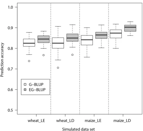
In the EG-BLUP model, both the additive and the additive3 additive epistatic relationship matrices were derived from molecular markers. If the markers under consideration are in linkage equilibrium (LE), the additive and additive3 ad-ditive terms in EG-BLUP* are orthogonal in the sense of Cockerham (1954), and hence the estimates of additive and epistatic effects are independent (Álvarez-Castro and Carlborg 2007). However, the assumption of linkage equi-librium may never be true in reality unless only a few loci sparsely distributed on the genome are considered. Hence,
we performed a simulation study to investigate whether linkage disequilibrium (LD) among markers, which causes nonorthogonality of the model, has an influence on the per-formance of EG-BLUP.
Our simulation was based on thefirst wheat data set [599 wheat lines with 1447 markers (Crossaet al.2010)] and the dent panel of the second maize data set [847 lines with 31,498 markers (Baueret al.2013)]. We simulated two sce-narios: (1) markers contributing to the trait are in LE and (2) markers contributing to the trait are in LD. In all cases, both additive and additive 3 additive epistatic effects were sim-ulated. The heritability was set to be 0.7. Details for the simulation procedure are presented inFile S1. We observed that the prediction accuracy of EG-BLUP was consistently higher than that of G-BLUP in both data sets and both sce-narios (Figure 1). Hence, we may conclude that LD among markers has low influence on the effectiveness of EG-BLUPvs.
G-BLUP.
Another factor that may affect the performance of EG-BLUP is inbreeding. In Henderson’s extended BLUP model (Henderson 1985), the derivation of the epistatic relation-ship matrix being the Hadamard square of the numerator relationship matrix depends on the assumption of random mating (Cockerham 1954), which may never hold for data from plant breeding. In our study, the marker-derived ep-istatic relationship matrix in EG-BLUP approximately equals the Hadamard square of the marker-derived addi-tive relationship matrix. This result relies only on the as-sumption that the marker additive and epistatic effects are independent. Maybe this assumption is more likely to hold in noninbred than in inbred populations. If this is true, the superiority of EG-BLUP over G-BLUP would be more pronounced for noninbred than for inbred popula-tions, provided that epistasis substantially contributed to the trait. An investigation of this problem is interesting but beyond the scope of this study. Nevertheless, our results in
Table 1 Cross-validated prediction accuracies and standard errors of three genomic selection models (genomic best linear unbiased prediction with additive relationship matrix (G-BLUP), extended G-BLUP with additive and additive3 additive relationship matrices (EG-BLUP), and reproducing kernel Hilbert space regression based on the Gaussian kernel (RKHS)] in four data sets
Data set Trait–environmente G-BLUP EG-BLUP RKHS
Wheat_1a GY_E1 0.50560.034 0.57160.029 0.57660.033
GY_E2 0.49360.034 0.50060.034 0.49960.034
GY_E3 0.37960.041 0.42160.035 0.42860.034
GY_E4 0.48460.033 0.52560.029 0.52660.034
Wheat_2b GY_drought 0.43560.058 0.44560.056 0.44460.054
GY_irrigated 0.53760.046 0.55060.046 0.55660.042
Maize_1c GY_drought 0.42960.044 0.44060.045 0.44960.043
GY_irrigated 0.53760.038 0.54660.037 0.54460.037
Maize_2ddent DMY 0.63260.030 0.62760.031 0.61960.032
Maize_2dflint DMY 0.65160.020 0.64960.021 0.64360.021
The highest prediction accuracy for each trait in each data set is underlined.
aData set previously described in Crossaet al.(2010); 599 lines and 1447 DArT markers were used. bData set previously described in Polandet al.(2012); 254 lines and 1576 SNP markers were used. cData set previously described in Crossaet al.(2010); 264 lines and 1135 SNP markers were used.
dData set previously described in Baueret al.(2013) and Lehermeieret al.(2014); 847 genotypes and 31,498 SNP markers were used for dent lines and 833 genotypes and
29,466 SNP markers were used forflint lines.
both simulation and empirical study indicated that EG-BLUP can be effectively applied to noninbred plant data.
Enhancing prediction accuracy across a biparental population through modeling epistasis
Previous studies have shown that prediction accuracy is im-paired when performing genomic selection across connected biparental populations (Zhaoet al.2012; Riedelsheimeret al.
2013). This may be explained at least partially by epistatic effects as the genetic relatedness across connected popula-tions may be better exploited by modeling epistasis in addi-tion to additive effects. Again we used a published maize data set (Bauer et al. 2013) and investigated whether the pre-diction accuracy across connected biparental families can be increased by modeling additive3additive epistasis. In our scenario, genotypic values of the lines in one family were predicted using lines from each of the other families. We compared the mean and maximal prediction accuracies for each family and observed no superiority for EG-BLUP and RKHS (including epistasis) compared with G-BLUP (ignor-ing epistasis; Figure 2). The sizes of the biparental popula-tions were small, ranging from 17 to 133. This small population size can substantially reduce prediction accuracy exploiting epistasis, as has been shown previously for QTL mapping (Carlborg and Haley 2004). In addition, maize as an outcrossing species is likely to be influenced only little by
additive 3 additive epistasis in contrast to selfing species (Garciaet al.2008). Therefore, it will be interesting to in-vestigate in future studies whether prediction accuracy across connected biparental populations can be improved, modeling epistasis using large biparental populations in selfing species.
Acknowledgments
We thank Yusheng Zhao and Timothy Sharbel for their valuable comments on the manuscript. We thank the authors in Crossa et al. (2010), Poland et al.(2012), Bauer et al.
(2013), and Lehermeier et al.(2014) for making their data sets publicly available. We are grateful to all reviewers and the editor for their helpful comments and suggestions, which greatly improved the manuscript. This study is based on published data sets. The authors have no conflicts of in-terest to declare.
Literature Cited
Álvarez-Castro, J. M., and Ö. Carlborg, 2007 A unified model for functional and statistical epistasis and its application in quanti-tative trait loci analysis. Genetics 176: 1151–1167.
Bauer, E., M. Falque, H. Walter, C. Bauland, C. Camisan et al., 2013 Intraspecific variation of recombination rate in maize. Genome Biol. 14: R103.
Figure 2 Mean and maximal prediction accuracies of maize lines in each family, using lines in each of the other families in the same heterotic group (dent or flint) as the estimation set. The prediction accuracies were evaluated using three different models [genomic best linear unbiased prediction (G-BLUP), extended G-BLUP with ad-ditive and adad-ditive 3additive relationship matrices (EG-BLUP), and reproducing kernel Hilbert space regression based on the Gaussian kernel (RKHS)].
Beavis, W. D., 1994 The power and deceit of QTL experi-ments: lessons from comparative QTL studies, pp. 250– 266 inProceedings of the Forty-Ninth Annual Corn and Sor-ghum Industry Research Conference, Vol. 1994, edited by D. B. Wilkinson. American Seed Trade Association, Wash-ington, DC.
Buckler, E. S., J. B. Holland, P. J. Bradbury, C. B. Acharya, P. J. Brownet al., 2009 The genetic architecture of maizeflowering time. Science 325: 714–718.
Cai, X., A. Huang, and S. Xu, 2011 Fast empirical Bayesian LASSO for multiple quantitative trait locus mapping. BMC Bioinfor-matics 12: 211.
Carlborg, Ö., and C. S. Haley, 2004 Epistasis: Too often neglected in complex trait studies? Nat. Rev. Genet. 5: 618–625. Carlborg, Ö., L. Jacobsson, P. Åhgren, P. Siegel, and L. Andersson,
2006 Epistasis and the release of genetic variation during long-term selection. Nat. Genet. 38: 418–420.
Cockerham, C. C., 1954 An extension of the concept of partition-ing hereditary variance for analysis of covariances among rela-tives when epistasis is present. Genetics 39: 859–882.
Comstock, R. E., and H. F. Robinson, 1952 Estimation of average dominance of genes, pp. 494–516 inHeterosis, edited by J. W. Gowen. Iowa State College Press, Ames, IA.
Crossa, J., G. de Los Campos, P. Pérez, D. Gianola, J. Burgueño et al., 2010 Prediction of genetic values of quantitative traits in plant breeding using pedigree and molecular markers. Genet-ics 186: 713–724.
Crossa, J., Y. Beyene, S. Kassa, P. Pérez, J. M. Hickey et al., 2013 Genomic prediction in maize breeding populations with genotyping-by-sequencing. G3 3: 1903–1926.
de Los Campos, G., D. Gianola, G. J. Rosa, K. A. Weigel, and J. Crossa, 2010 Semi-parametric genomic-enabled prediction of genetic values using reproducing kernel Hilbert spaces methods. Genet. Res. 92: 295–308.
Fisher, R. A., 1918 The correlation between relatives on the sup-position of Mendelian inheritance. Trans. R. Soc. Edinb. 52: 399–433.
Garcia, A. A. F., S. Wang, A. E. Melchinger, and Z. B. Zeng, 2008 Quantitative trait loci mapping and the genetic basis of heterosis in maize and rice. Genetics 180: 1707–1724. Gianola, D., and J. B. van Kaam, 2008 Reproducing kernel Hilbert
spaces regression methods for genomic assisted prediction of quantitative traits. Genetics 178: 2289–2303.
Gianola, D., R. L. Fernando, and A. Stella, 2006 Genomic-assisted prediction of genetic value with semiparametric procedures. Ge-netics 173: 1761–1776.
Gianola, D., G. Morota, and J. Crossa, 2014 Genome-enabled prediction of complex traits with kernel methods: What have we learned? in Proceedings of the Tenth World Congress of Genetics Applied to Livestock Production. Vancouver, BC, Canada. Available at:https://asas.org/docs/default-source/ wcgalp-proceedings-oral/212_paper_10331_manuscript_1636_0. pdf?sfvrsn=2.
Habier, D., R. L. Fernando, and J. C. M. Dekkers, 2007 The impact of genetic relationship information on genome-assisted breeding values. Genetics 177: 2389–2397.
Hayes, B. J., P. J. Bowman, A. J. Chamberlain, and M. E. Goddard, 2009 Genomic selection in dairy cattle: progress and chal-lenges. J. Dairy Sci. 92: 433–443.
Henderson, C. R., 1975 Best linear unbiased estimation and pre-diction under a selection model. Biometrics 31: 423–447. Henderson, C. R., 1985 Best linear unbiased prediction of
non-additive genetic merits. J. Anim. Sci. 60: 111–117.
Howard, R., A. L. Carriquiry, and W. D. Beavis, 2014 Parametric and non-parametric statistical methods for genomic selection of traits with additive and epistatic genetic architectures. G3 4: 1027–1046.
Hu, Z., Y. Li, X. Song, Y. Han, X. Caiet al., 2011 Genomic value prediction for quantitative traits under the epistatic model. BMC Genet. 12: 15.
Huang, A., S. Xu, and X. Cai, 2014 Whole-genome quantitative trait locus mapping reveals major role of epistasis on yield of rice. PLoS One 9: e87330.
Jannink, J. L., A. J. Lorenz, and H. Iwata, 2010 Genomic selection in plant breeding: from theory to practice. Brief. Funct. Ge-nomics 9: 166–177.
Lehermeier, C., N. Krämer, E. Bauer, C. Bauland, C. Camisanet al., 2014 Usefulness of multiparental populations of maize (Zea maysL.) for genome-based prediction. Genetics 198: 3–16. Levi, H., 1968 Polynomials,Power Series and Calculus. Van
Nos-trand, Princeton, NJ.
Lorenzana, R. E., and R. Bernardo, 2009 Accuracy of genotypic value predictions for marker-based selection in biparental plant populations. Theor. Appl. Genet. 120: 151–161.
Lynch, M., and B. Walsh, 1998 Genetics and Analysis of Quantita-tive Traits. Sinauer Associates, Sunderland, MA.
Mackay, T. F., 2014 Epistasis and quantitative traits: using model organisms to study gene-gene interactions. Nat. Rev. Genet. 15: 22–33.
Meuwissen, T. H. E., B. J. Hayes, and M. E. Goddard, 2001 Prediction of total genetic value using genome-wide dense marker maps. Genetics 157: 1819–1829.
Morota, G., and D. Gianola, 2014 Kernel-based whole-genome prediction of complex traits: a review. Front. Genet. 5: 363. Muñoz, P. R., M. F. Resende, S. A. Gezan, M. D. V. Resende, G. de
los Camposet al., 2014 Unraveling additive from nonadditive effects using genomic relationship matrices. Genetics 198: 1759–1768.
Pérez-Rodríguez, P., D. Gianola, J. M. González-Camacho, J. Crossa, Y. Manès et al., 2012 Comparison between linear and non-parametric regression models for genome-enabled pre-diction in wheat. G3 2: 1595–1605.
Phillips, P. C., 2008 Epistasis—the essential role of gene inter-actions in the structure and evolution of genetic systems. Nat. Rev. Genet. 9: 855–867.
Poland, J., J. Endelman, J. Dawson, J. Rutkoski, S. Wu et al., 2012 Genomic selection in wheat breeding using genotyping-by-sequencing. Plant Genome 5: 103–113.
Riedelsheimer, C., J. B. Endelman, M. Stange, M. E. Sorrells, J. L. Janninket al., 2013 Genomic predictability of interconnected biparental maize populations. Genetics 194: 493–503. Rutkoski, J., J. Benson, Y. Jia, G. Brown-Guedira, J. L. Jannink
et al., 2012 Evaluation of genomic prediction methods for fu-sarium head blight resistance in wheat. Plant Genome 5: 51–61. Su, G., O. F. Christensen, T. Ostersen, M. Henryon, and M. S. Lund, 2012 Estimating additive and non-additive genetic variances and predicting genetic merits using genome-wide dense single nucleotide polymorphism markers. PLoS One 7: e45293. Tian, F., P. J. Bradbury, P. J. Brown, H. Hung, Q. Sun et al.,
2011 Genome-wide association study of leaf architecture in the maize nested association mapping population. Nat. Genet. 43: 159–162.
VanRaden, P. M., 2008 Efficient methods to compute genomic predictions. J. Dairy Sci. 91: 4414–4423.
Wang, D., I. S. El-Basyoni, P. S. Baenziger, J. Crossa, K. M. Eskridge et al., 2012 Prediction of genetic values of quantitative traits with epistatic effects in plant breeding populations. Heredity 109: 313–319.
Wittenburg, D., N. Melzer, and N. Reinsch, 2011 Including non-additive genetic effects in Bayesian methods for the prediction of genetic values based on genome-wide markers. BMC Genet. 12: 74.
genetic interaction networks in sugar beet. Theor. Appl. Genet. 123: 109–118.
Xu, S., 2007 An empirical Bayes method for estimating epistatic effects of quantitative trait loci. Biometrics 63: 513–521. Yang, J., B. Benyamin, B. P. McEvoy, S. Gordon, A. K. Henderset al.,
2010 Common SNPs explain a large proportion of the herita-bility for human height. Nat. Genet. 42: 565–569.
Zhao, Y., M. Gowda, W. Liu, T. Würschum, H. P. Maurer et al., 2012 Accuracy of genomic selection in European maize elite breeding populations. Theor. Appl. Genet. 124: 769–776. Zhao, Y., M. F. Mette, and J. C. Reif, 2015 Genomic selection in
hybrid breeding. Plant Breed. 134: 1–10.
Appendix: A Proof of the Equivalence Between EG-BLUP and EG-BLUP* When the Number of Markers Is Large
Let us start with the EG-BLUP* model (Equation 5). Let a be the p-dimensional vector of the ai’s and v be the
pðp21Þ=2-dimensional vector of the vij’s. Let U be the n3pðp21Þ=2 matrix whose columns are given by the vectors ðWiWjÞ:Then Equation 5 can be simply written as
y¼1nmþWaþUvþe;
with assumptionsaNð0;Iðs2
1=gÞÞ;vNð0;Ið2s22=g2ÞÞ;andeNð0;Is2eÞand all covariance terms are zero. Then we have
V¼varðyÞ ¼WW9
g s21þ 2UU9
g2 s 2
2þIs2e: (A1)
The matrixUU9is ann3nmatrix whoseði;jÞentry is given by
X
1#k,s#p
ui;ksuj;ks¼
X
1#k,s#p
wikwiswjkwjs¼1 2
X
1#k;s#p
wikwiswjkwjs2
Xp
k¼1 w2ikw2jk 0
@
1 A
¼1 2
Xp
k¼1 wikwjk
! Xp
s¼1 wiswjs
!
2X
p
k¼1 w2ikw2jk
" #
:
Then it is easy to deduce that
UU9¼1
2
WW9#WW92ðW#WÞðW#WÞ9 :
Hence we have
2UU9
g2 ¼G#G2
ðW#WÞðW#WÞ9
g2 :
Now we claim that
lim p/N
2UU9
g2 ¼plim/NG#G;
which means that whenpis very large, we can approximately treat2UUg29G#G:For this purpose we need only to prove
lim p/N
ðW#WÞðW#WÞ9
g2 ¼0: (A2)
In fact, theði;jÞth entry of the matrixðW#WÞðW#WÞ9=g2 is
tij¼
Xp k¼1w
2 ikw2jk
4 Xpk¼1pkð12pkÞ 2¼
Xp
k¼1ðxik22pkÞ 2ð
xjk22pkÞ2
4 Xpk¼1pkð12pkÞ
2 : (A3)
Note that we always exclude monomorphic markers in the analyses. So we can assume thatp0,pk,12p0;wherep0is the threshold of minor allele frequency in the quality control (e.g.,p0¼0:01 or 0:05). Then the numerator of (A3) is a sum of
ppositive numbers, each belonging to the interval½0;16ð12p0Þ2;while the denominator is a sum ofp2positive numbers, each in the interval½4p20ð12p0Þ2;
0:25:Thus we have
0# lim
p/Ntij#plim/N
16ð12p0Þ2p 4p20ð12p0Þ2p2
¼ lim p/N
4
p2 0p
which proved (A2).
Hence (A1) is simplified to the following:
VGs21þ ðG#GÞs22þIs2e:
The right-hand side of the above formula is exactly the same as the variance–covariance matrix varðyÞ for Equation 3 in EG-BLUP.
By the results of Henderson (1975), the BLUPs ofaandvare given by
^
a¼s 2 1
g W9V21ðy21nm^Þ; ^v¼ 2s2
2 g2 U9V2
1ð
y21nm^Þ; (A4)
where
^
m¼ 19nV21y
19nV211n: (A5)
On the other hand, the BLUPs ofg1andg2in the EG-BLUP model are given by
^
g1¼s21GV21ðy21nm^Þ; ^g2¼s22ðG#GÞV21ðy21nm^Þ; (A6) wherem^is the same as in (A5) as we have proved that the matricesV¼varðyÞin EG-BLUP and EG-BLUP* are the same.
GENETICS
Supporting Information
www.genetics.org/lookup/suppl/doi:10.1534/genetics.115.177907/-/DC1
Modeling Epistasis in Genomic Selection
Yong Jiang and Jochen C. Reif
![Table 1 Cross-validated prediction accuracies and standard errors of three genomic selection models (genomic best linear unbiasedprediction with additive relationship matrix (G-BLUP), extended G-BLUP with additive and additive 3 additive relationship matrices(EG-BLUP), and reproducing kernel Hilbert space regression based on the Gaussian kernel (RKHS)] in four data sets](https://thumb-us.123doks.com/thumbv2/123dok_us/1537054.1188522/5.603.49.556.79.199/validated-prediction-accuracies-unbiasedprediction-relationship-relationship-reproducing-regression.webp)