ABSTRACT
BERGLUND, ANDREW DAVID. An Iterative Simulation and Mathematical Programming Optimization Approach to Leak Detection in Water Distribution Systems. (Under the
direction of Dr. Kumar Mahinthakumar and Dr. E. Downey Brill, Jr.)
Real water losses from leaks present a serious and growing challenge in water
resources planning. As the national water infrastructure ages, pipe walls and connections fail
under stress and give way to leaks, a major source of water loss. Not only do leaks equate to
lost revenue for utilities, but they can also critically alter system operations. In the extreme
case, water discharged from an unmetered source, such as a leak, can reduce the available
head in a water distribution system drastically enough to cut consumers off from access to
water. Finding and repairing leaks can be difficult as even a substantial leak can potentially
show no manifest signs. Traditional leak detection methods, such as acoustic surveys, require
significant resources and specialized training.
This research employs mathematical programming methods, Linear Programming
and Mixed Integer Programming, in a simulation-optimization framework to explore an alternative leak detection methodology based on pressure measurements. Simulated “real”
pressure data were obtained for model networks with and without leaks present. Then single,
independent leaks were simulated at each network node. The method determines a linear combination of these leaks that most closely approximate the pressure pattern for “real”
leaks. Steady state and time-varying models were used to test the method. Results are
presented to emphasize the method’s effectiveness under different conditions. This method’s
potential lies in the fact that it is not intended to replace traditional leak detection methods.
Rather, it is meant to work in concert with available methods to more accurately and
An Iterative Simulation and Mathematical Programming Optimization Approach to Leak Detection in Water Distribution Systems
by
Andrew Berglund
A thesis submitted to the Graduate Faculty of North Carolina State University
in partial fulfillment of the requirements for the Degree of
Master of Science
Civil Engineering
Raleigh, North Carolina
2014
APPROVED BY:
_______________________________ Dr. Detlef Knappe
Dr. Kumar Mahinthakumar Co-Chair of Advisory Committee
BIOGRAPHY
Andrew David Berglund is the youngest of five children. He was born in Aurora,
Colorado, and, prior to moving to North Carolina for graduate school, has lived the majority
of his life in Colorado. He attended the University of Colorado at Boulder for his
undergraduate education where he obtained a Bachelor of Arts in Molecular, Cellular, and
Developmental Biology and double-majored with Biochemistry. He now lives in Raleigh,
North Carolina with his wife Emily where he plans to use his education to the betterment of
ACKNOWLEDGEMENTS
I would foremost like to thank my wife for her support while writing this document. I
would also like to thank both of my co-chairs Dr. Kumar and Dr. Brill for taking me as a
TABLE OF CONTENTS
LIST OF TABLES ... v
LIST OF FIGURES ... vi
1. Introduction ... 1
2. Background ... 3
3. Methodological Development ... 4
3.1. Initial Sensitivity Analysis ... 4
3.2. Method Overview ... 10
3.3. Simulation-Optimization Framework ... 12
3.4. Linear Programming Formulation ... 14
3.5. Mixed Integer Programming Formulation ... 17
3.6. Algorithm Overview ... 19
3.7. Hanoi Network ... 21
3.8. Net3 Network ... 22
4. Results and Discussion ... 32
4.1. Hanoi Network ... 32
4.2. Net3 Network ... 36
5. Conclusion ... 48
LIST OF TABLES
Table 1 - Diurnal demand pattern for residential nodes in Net3. ... 24
Table 2 - Objective value by method and iteration. ... 36
Table 3 - Average objective value for each sub-period length over 50 trials. ... 39
Table 4 - Average solution error over 50 trials by sub-period length. ... 39
LIST OF FIGURES
Figure 1 - The Micropolis Network. Lines represent the pipe network which connects the network’s nodes. Each node is represented as a dot. ... 5
Figure 2 – The average summed pressure indicator for the Micropolis network by leak
coefficient. ... 8
Figure 3 – A comparison of summed pressure indicator values by leak magnitude between
two simultaneously simulated leaks and two leaks at the same locations simulated
independently. ... 9
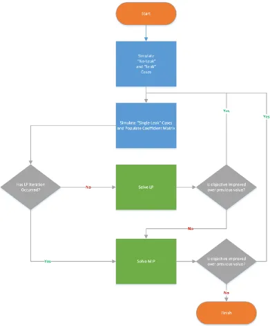
Figure 2 - Flow through combined iterative approach. Blue color represents a stimulation
process. Green represents an optimization process... 20
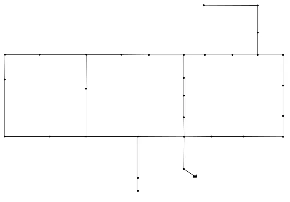
Figure 5 - The Hanoi network. Lines represent the pipe network which connects the
network’s nodes. Each node is represented as a dot. ... 21
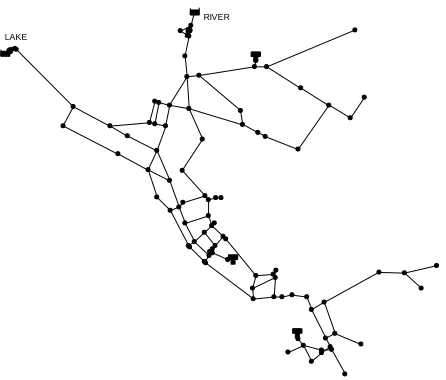
Figure 6 - The Net3 network. Lines represent the pipe network which connects the network’s
nodes. Each node is represented as a dot. ... 23
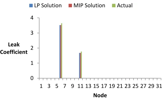
Figure 7 - Single run comparison of LP and MIP run independently. ... 33
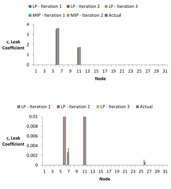
Figure 8 - (a-top) Leak coefficient solution for each iteration of the combined iterative
method. (b-bottom) The same solution magnified along the y-axis to show small leaks
present in LP solutions. ... 34
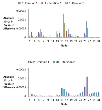
Figure 9 – Absolute pressure error by node for each iteration of (a-top) the LP and (b-bottom)
Figure 10 - Results from the first sub-period of the 24-hour simulation for the (a) 1-hour, (b)
2-hour, (c) 3-hour, (d) 4-hour, (e) 6-hour, (f) 8-hour, (g) 12-hour, and (h) 24-hour
sub-periods. Red squares indicate leak coefficient magnitudes in the observed case. Blue circles
indicate leak coefficient magnitudes from the simulated case solution. ... 38
Figure 11 - Heat map of raw results for single trial of combined iterative approach. Actual
leak locations indicated by red color in right-hand row labels. ... 42
Figure 12 - Heat map of solutions within 20 percent of lowest objective sub-period for a
single trial. Actual leak locations indicated by red color in right-hand row labels. ... 44
Figure 13 - Heat map of the lowest objective solution for each sub-period length and the
same trial. Actual leak locations indicated by red color in right-hand row labels. ... 45
Figure 14 - Time-normalized objective values for 24 1-hour solutions, evaluated at every
hour. ... 46
Figure 15 - The final reduced heat map with outlier solutions removed. Actual leak locations
1.
Introduction
Utilities across the United States face an aging water infrastructure in which stressed
pipes frequently break. These breakages constitute a major portion of real water losses—a
term popularized by the American Water Works Association (AWWA)—and are a growing
concern for water utilities. These real loses are “the physical losses of water from the
distribution system, including leakage and storage overflows. These losses inflate the water
utility's production costs and stress water resources since they represent water that is
extracted and treated, yet never reaches beneficial use” (AWWA, 2012). This major issue is
further compounded by predicted future water scarcity brought on by population growth and
climate change. Historically, finding and fixing leaks has been challenging. Large leaks may
intuitively seem to be the largest contributors to water loss, but these leaks often manifest in
visible above-ground ways, often with a large enough impact that they are found and fixed
quickly. Small leaks can have a profound impact over time on water loss because they often
remain unobservable from the surface. Traditional leak detection methods are costly, require
experienced operators, and rely on many variables such as pipe material and diameter. A
cost-effective and consistent method to reliably detect leaks using readily available data is
imperative.
To date, simulation based leak detection methodologies have not reached the maturity
required for mainstream adoption. Previous research in the field has focused largely on the
analysis of pressure transients, short-burst pressure waves induced by pumping and changes
but not when considering an entire water distribution network. Work remains to be done in
extending these methods to use in full water distribution networks.
Presented here is a simulation-optimization leak detection method that considers an
entire network at one time. The method solves the inverse problem of detecting the location
and magnitude of unknown leaks in a water distribution system by finding the linear
combination of independent leaks that minimizes the pressure difference between simulated
2.
Background
Leak detection methods usually fall in one of two categories: physical methods and
computer-based methods. Physical methods, which are presently the most used, rely on the
ability to distinguish the acoustic signature of leaks. Many utilities use acoustic surveys as a
major component of their water audit strategy. Computer-based methods use a model of the
water system to simulate the changes a leak produces in the water system.
Physical methods rely on acoustic devices to detect leaks. A leak can be thought of as
a constantly “on” demand sink. Above-ground acoustic surveys seek to find areas where
water appears to be flowing when known withdrawals are limited or, by way of a valve, shut
off entirely. The ability to detect the flow of water through a broken pipe is largely dependent
on the pipe material, the leak’s size, and the subjectivity of the operator. Modern methods
make use of in-line acoustic sensors that are released into the network and capture sound data
as they travel. Sensor data are analyzed to detect anomalous signatures corresponding to
potential leaks. The use of ground penetrating radar has also gained popularity for more
shallow networks (Mutikanga, 2013).
Computer-based methods make use of hydraulic models to simulate leaks. Many
methods seek to detect pressure transients, short-burst pressure waves produced at a location
of disrupted flow during regular pressure or flow velocity changes. Other methods seek to
minimize the difference between simulated leaks and observed data. These methods often use
heuristic search methods as the complex effects of leaks in water networks are not well
3.
Methodological Development
3.1. Initial Sensitivity Analysis
An initial series of experiments was conducted to determine if an approximately
linear relationship between pressure change and leak magnitude could be exploited. Once
this relationship was established the pressure difference between a simulation with multiple
simultaneous leaks and multiple simulations with single leaks were compared to see how
effectively multiple leaks could be modeled using a linear combination of single leak
scenarios. Simulations were run using EPANET (Rossman, 2000) and the Micropolis
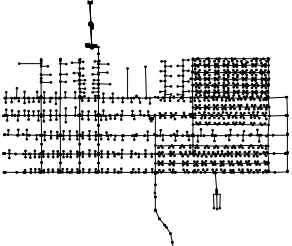
network (Brumbelow, 2007), as seen in Fig. 1. The Microplis network represents a small city
of approximately 5,000 residents and contains 1236 nodes—458 of which are demand
nodes—575 mains, 486 service and hydrant connections, 197 valves, 28 hydrants, 8 pumps, 2
Figure 1 - The Micropolis Network. Lines represent the pipe network which connects the network’s nodes. Each node is represented as a dot.
A simple metric was developed to study the pressure response in a network due to the
introduction of a leak. The pressure difference between a no-leak and leak scenario was
summed for all nodes, over all time steps in the simulation to obtain a single summed
pressure response indicator as shown in Equation 1.
, ,
0 0
(
)
j t j t
d n
no leak leak t j
P
p
p
(1)Where is the summed pressure response indicator, is the pressure at node j and
time t in the no-leak case and is the pressure at node j and time t in the leak case. The
pressure difference is summed over the network's n nodes at each hourly time step and
incrementally larger magnitude to determine if pressure response depends linearly on leak
magnitude. Once this relationship was established, two leak locations were selected and a
two-leak case and two single-leak cases were simulated. The indicator was calculated for
each, and the two single-leak indicators were summed and compared to the two-leak
indicator to determine if multiple leaks could be approximated by assessing a combination of
single leaks.
Leaks are modeled in EPANET as emitters and follow Equation 2.
Q
cP
(2)Where is a volumetric flow rate, is the leak or discharge coefficient, is pressure, and
is a pressure exponent, set at 0.5 for this study. In EPANET leaks must be modeled at a
network node, not in a link, or pipe, between nodes. When flow is measured in gallons per
minute (gpm) and pressure in pounds per square inch (psi), the leak coefficient c can be
expressed in units of , expressed as the flow through a leak due to a 1 psi pressure drop. The flow rate, and thus the excess demand caused by an individual leak is pressure sensitive
and the true quantitative demand of the leak is difficult to control due to regular pressure
fluctuations. The most direct control of a leak’s magnitude is exercised by changing the
value, or the leak coefficient. The pressure difference between a no-leak and leak scenario is
also a function of the leak coefficient. All subsequent references to leak magnitude are
The preliminary work presented here indicates that, in a rough sense, the pressure
change indicator responds linearly to an increase in leak magnitude. As a leak increases in
size, more water is lost, and less water remains in the pressured pipe system. With less water,
the system experiences a pressure drop. The summed pressure indicator increases linearly as
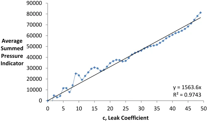
the leak coefficient increases as seen in Fig. 2. Each point represents the network average for
a particular c value, obtained by simulating a leak at each of the network’s nodes and then
taking an average indicator value. The non-linearity exhibited for low c values is possibly
Figure 2 – The average summed pressure indicator for the Micropolis network by leak coefficient.
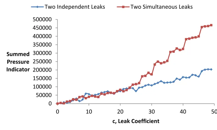
The linear relationship between leak coefficient and pressure was explored further by
introducing multiple leaks. The summed pressure indicator was obtained over a range of leak
coefficient values for the two-leak case, modeled as two simultaneous leaks and two
independently simulated leaks, placed at each of the simultaneous leak locations. The
indicators obtained from the two independent leaks were summed and compared to the
indicator obtained from the two simultaneous leaks as seen in Fig. 3.
y = 1563.6x R² = 0.9743 0
10000 20000 30000 40000 50000 60000 70000 80000 90000
0 5 10 15 20 25 30 35 40 45 50
Average Summed Pressure Indicator
Figure 3 – A comparison of summed pressure indicator values by leak magnitude between two simultaneously simulated leaks and two leaks at the same locations simulated independently.
In the network tested, the superposition principle holds for leaks with coefficients
below an approximate value of 25. The finding that two independent leaks, when considered
together closely approximate two simultaneously existing leaks led to the consideration of a
linear method for leak detection. While conducting preliminary trials the effect of complex
pumping rules on pressure change in the leak case was noted. The introduction of a single
small leak in a network with pumps can alter the pumping schedule enough to register
positive pressure changes in a leak case and subsequent single leak simulations when
compared to the no-leak case. This effect is dependent on the pump rules that govern the
model, typically those that are responsive to tank levels. A set of rules that are purely time
dependent should be insensitive to the presence of a leak. This positive pressure change is not
necessarily fatal to the model formulation, as the objective function seeks to minimize the
0 50000 100000 150000 200000 250000 300000 350000 400000 450000 500000
0 10 20 30 40 50
Summed Pressure Indicator
c, Leak Coefficient
sum of the absolute pressure differences, but the decision to begin with a simpler water
network was made.
3.2. Method Overview
A mathematical programming based method using a coupled simulation-optimization
framework was developed to find both the location and magnitude of simultaneously existing
unknown leaks in a water distribution system (WDS). This work hypothesizes that the
interactions of multiple leaks within a WDS have a complex non-linear effect that can be
approximated as linear. This hypothesis is supported by preliminary sensitivity analyses
which indicate a linear response of pressure dependence with leak magnitude represented as
a leak coefficient, c. Linear Programming (LP) is used to minimize differences in simulated
and observed pressure readings. For this study, however, the “observed”, or “real-world,”
data were synthetically generated using simulated leaks in idealized model networks. In this
work, simulated pressure readings are generated from the modeled water network without
leaks, referred to as the "no-leak" case, and the readings obtained with leaks having
randomized locations and magnitudes are termed the "leak" case. The use of simulated data
using small, simplified model networks is considered a first step in method development and
treated as proof of concept. The no-leak case and leak case are meant to reflect the normal
operations of a WDS before and after the introduction of leaks. In the networks tested, the
flow of water into the network is limited only by pump specifications. The water source does
Of specific interest in this study is the pressure change experienced inside a
pressurized water network due to the introduction of a leak. Hydraulic simulations are
performed to obtain pressure data at regular intervals, collected for both cases at network
nodes specifically chosen as pressure sensors. As this is an inverse problem, the pressure
change due to the introduction of leaks does not explicitly reveal the location or magnitude of
the introduced leaks; a model is needed to select candidate leaks that create a pressure change
signature close to that introduced by leaks in the leak case. A series of additional simulations
are conducted to determine the pressure change caused by a single leak at each of the
network's nodes. In each simulation a single small leak is placed at one of the networks nodes
and pressure data is collected. This process is repeated until a leak at each network node has
been simulated. The obtained pressure data is then compared to the base case to obtain a
pressure difference. The collected data constitutes a library of the network’s pressure
response coefficients to a leak at each possible location.
An LP model is then built and optimized to determine the linear combination of
single simulated leaks that best emulate the change in pressure between the no-leak case and
the leak case. The LP selects a combination of leaks that minimize the objective function, the
sum of the absolute error between the pressure difference in the leak case and the linear
combination of simulated leaks. A series of linear constraints assure a solution that yields the
estimated leak magnitudes that minimize the pressure error. An optimal solution to the LP is
passed back to the simulation and used to update the magnitudes of the simulated leaks. The
optimized again. This iterative process continues until the LP generates a solution that does
not improve the objective function. This solution is discarded and the last solution to lower
the objective function is used to continue. The number of estimated leaks in this solution
greater than a preselected parameter threshold value is counted. This number is then used in a
polishing step in which additional binary constraints are added to the LP formulation to
create a Mixed Integer Programming (MIP) model.
The MIP model allows the user a level of control over the solutions obtained by
restricting the total number of searched-for leaks. The proposed method uses the previously
calculated total number of leaks in the LP solution above a threshold to determine the
number of leaks allowed in an MIP solution. This limit is readily adjustable and can be tuned
if additional system information is known or to observe how solutions respond as the number
of searched-for leaks is changed. Once the MIP is constructed, it is solved iteratively in the
same fashion as the LP until there is again no improvement in the MIP objective error. The
overall method is heuristic in the sense that there is no proof of convergence to a good
solution, but as shown below it performs well on the test problems to date.
3.3. Simulation-Optimization Framework
The simulation-optimization framework developed in this research uses the EPANET
Programmer’s Toolkit functions in concert with Gurobi Optimizer 5.5 (Gurobi Optimizer
Reference Manual, Version 5.5, 2013). All hydraulic simulations are performed using
Leak locations and magnitudes for the leak case are selected using pseudorandom number
generation. Information regarding leaks in the leak case is used for assessment of LP and
MIP-generated solutions. The model is otherwise run as if this information is unavailable. A
hydraulic simulation is carried out for each of the network’s nodes, with a small leak
simulated at that node. Pressure data are recorded at the same pressure reporting nodes in the
no-leak and leak cases and the pressure differences at the sensors are determined (perfectly
performing sensors are assumed). The pressure differences are likewise determined between
the no-leak case and each simulated-leak case. These data are used to populate the coefficient
matrices for the LP problem.
The LP is constructed using the Gurobi C language interface functions. Each Gurobi
LP model is optimized within the Gurobi Optimization environment. Once the environment
is initialized, a specific model can be populated. The model is initiated by selecting the
quantity, type, and objective coefficient for all of the model’s variables. Linear constraints
are built for each row of the constraint coefficient matrix. The C Gurobi implementation
requires that a constraint is built using only non-zero constraints coefficients. Care is required
to not read in zero constraint values as the full constraint matrix for this problem includes
two Identity sub-matrices. Once the objective function and all constraints are set, the model
is optimized. The solution obtained for the LP problem contains the estimated values for
each node in the network, and the error at each pressure sensor between the simulated and
leak case. New hydraulic simulations are run using the solution's leak coefficient values. The
simulation pressures and the LP is rebuilt and resolved. This iterative process continues until
the objective function, the minimization of pressure error, no longer decreases.
3.4. Linear Programming Formulation
The LP being solved is formulated as an L1-Approximation problem, in which the
sum of absolute differences between the simulated and observed pressure readings at all m
pressure sensors is minimized. This can be expressed as an LP problem, shown in Equation
3.
1
1
minimize
(
)
subject to
(
)
i m i i i n i
j i i obs
j j
y
y
p
x
y
y
p
i
c
x (3)Where yi and yi are variables assigned for each of the m pressure sensors that capture
either the positive or negative difference in pressure between the simulated and observed
pressure, respectively; i j
p c
is the pressure response coefficient at pressure sensor i for a leak
with coefficient cj simulated at node j; xj is the leak coefficient variable being solved for at
node j;
i
obs
p is the observed pressure at sensor i.
In this research, an equivalent matrix formulation of the L1-norm minimization problem
1
( ) 1
1
1
1
(m ) 1
1 11 1 1 1
minimize
subject to
,
,
0
0
,
,
1
1
,
i i T i i m n n ni obs sim
m m
n
n
n
m mn
n m n
x
x
c
x
y
y
p
p
y
p
p
c
c
p
p
c
c
d x
Ax
b
x
x
x
y
y
d
A
1 1 0 02 (m ) 2 1
0 1
,
,
i ij m m sim ij ij j obsm n m
obs m
p
p
p
c
c
p
p
p
p
A
-I
b
A
b
b
Where is the vector containing the variable vectors and , is the leak coefficient for
each of the n nodes, and is the error term for each of the m pressure sensors,
respectively. The vector contains the objective coefficients for the LP objective function.
The objective is to minimize the sum of the pressure error terms. Accordingly, all variables
representing leak coefficients receive a zero coefficient, and all pressure error terms receive a
coefficient of one. The m x n matrix is a response matrix containing the pressure difference
between the no-leak case, , and the simulated cases, , normalized by leak magnitude, for i=1…m and j=1…n. Each row of this matrix corresponds to a single pressure sensor.
Each column corresponds to a leak at a single node in the network. The matrix is the
constraint matrix for the LP and is built using the previously described response matrix and
an identity matrix I. Each row of this matrix corresponds to the coefficients for the left hand
side of a single linear inequality constraint. Two constraints are created for each pressure
sensor represented in the matrix, one from positive and one from negative . This
creates a positive and negative bound and is done to obtain the absolute error. Each constraint
can be interpreted as the requirement that the sum of each leak coefficient at each node,
multiplied by its corresponding response matrix value and the pressure error term at the
current pressure sensor must be less than or equal to the difference in pressure between the
no-leak case and the leak case. The vector contains the pressure difference between the
no-leak case, , and the leak case, , at pressure sensor i, i=1…m. The vector contains
LP returns the vector which contains the estimated leak coefficient for every network node
and the pressure error term for every pressure sensor.
3.5. Mixed Integer Programming Formulation
The Mixed Integer Programming (MIP) formulation is used to refine the solution
obtained from the LP problem. The MIP problem consists of the same objective function and
linear inequality constraints as the LP, while further constraining the number of permissible
leaks. The limit on the number of leaks is obtained by summing the number of leak
coefficients in the best LP solution that meet or exceed a predefined threshold. The number
of leak coefficients allowed in the MIP solution is forced to be at or below this limit. The
MIP achieves this by introducing binary variables, those that can be either 0 or 1, into the
model. The additional MIP constraints are shown in Equation 5.
1
0,
1...
N,
0,1
i i
n
i i
x
Mz
i
m
z
z
(5)Where is the leak coefficient solution for the node i, is the corresponding binary
variable for that node and , called “big M”, is used to bound the leak coefficients. Through
this constraint any node with a corresponding binary variable equal to zero is itself forced to
zero. The leak coefficient at a node with an associated binary variable equal to one must be
less than . The sum of the binary variables is also limited to be equal to or less than , the
maximum number of allowed leaks. The MIP is then solved in a similar manner to the LP
as in the LP and in addition, n binary variable values, one for each network node. MIP
problems can, at worst, introduce 2n more solution combinations due to the addition of n new
variables, each with possible values zero or one. Although modern MIP algorithms, including
the proprietary version used by Gurobi, have a series of techniques to reduce the time to
optimality, MIP problems can be difficult to solve. To help combat this difficulty, each MIP
iteration is given a valid starting combination of binary variables that will produce a feasible
solution. This gives a feasible upper bound on the objective that can be used to eliminate
solutions with higher objective values. The starting solution for the first MIP is generated
from the best LP solution. This starting solution is not guaranteed to be feasible, but offers a
starting point for the search. Each successive MIP starting solution is used from the previous
MIP iterations solution. The MIP is solved iteratively, passing solutions back to the
simulation in the same way described for the LP. This continues until an MIP solution is
obtained that does not improve the objective function. The final MIP solution that improves
3.6. Algorithm Overview
The overall flow of the algorithm is expressed in the following steps and the flow chart
shown in Fig 4.
Start
Step 1. Set current objective value to a high value (e.g., 9999). Step 2. Set
Step 3. Simulate no-leak and leak cases. Step 4. Populate the and vector
Step 5. Simulate simulated case for n nodes Step 6. Populate the and matrices
Step 7. Set previous objective value <- current objective value Step 8a. Generate and solve LP
If (current objective value - previous objective value) < 0
Step 8b. If Set Return to Step 5.
Step 9. Set current objective value to a high value (e.g., 9999). Step 10. Set previous objective value <- current objective value Step 11. Simulate simulated case for n nodes
Step 12. Populate the and matrices
Step 13a. Generate and solve MIP
If (current objective value - previous objective value) < 0
Step 13b. If Set Return to Step 10.
3.7. Hanoi Network
The Hanoi EPANET network (Hanoi) shown in Fig. 5 is a simple, gravity-fed 31
node, skeletonized network modeled after Hanoi, Vietnam. The EPANET input file
represents a single steady state simulation without time varying demand. The pipe diameters
used were determined from a published network design (Savic, 1997). The entire system is
fed from a single reservoir with 100 meters of available head. Hanoi was selected as the first
network to test the linear mathematical programming formulation. The network’s small size
(there are three large pipe loops), lack of time variance, and absence of pumps offered a
problem with reduced complexity to test if it was possible to model leaks in a linear fashion.
Figure 5 - The Hanoi network. Lines represent the pipe network which connects the network’s nodes. Each node is represented as a dot.
Pressure data were obtained from all nodes for tests run with the Hanoi network. The
of improving the overall method easier. For all Hanoi experiments the LP problem was
solved iteratively until there was no improvement in objective value. The lowest objective
solution was used to determine the binary limit on the number of allowable leaks in the MIP
formulation. The MIP was then solved iteratively until there was no longer improvement in
the objective.
3.8. Net3 Network
The EPANET Net3 network, shown in Fig. 6 was selected as a network with
additional complexity, while maintaining enough simplicity to simulate and solve quickly.
The Net3 network comes packaged with EPANET and consists of 92 junction nodes, two
Figure 6 - The Net3 network. Lines represent the pipe network which connects the network’s nodes. Each node is represented as a dot.
The network was modified to run for 96 hours, including a three day (72-hour) warm-up
period. During the warm-up period, the simulation runs normally, but no data are collected. It
is intended to allow the network’s hydraulics to equilibrate. The final 24-hour period is used
for evaluation. The original EPANET input file consists of a 24-hour simulation in which
water no longer comes from the lake source after hour fifteen. This rule was left intact,
making the network effectively a single-source network for the period of evaluation. There is
a single pump that delivers water from the river source. This pump has a simple control
scheme; it turns on when the height of water in Tank 1 is below 17.1 feet and off when the
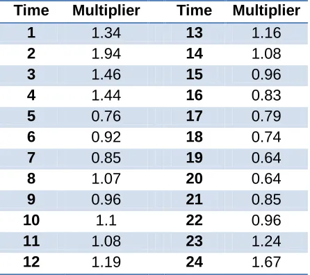
height of water in Tank 1 is above 19.1 feet. All but four of the junction nodes follow the
diurnal demand multiplier pattern shown in Table 1. LAKE
Table 1 - Diurnal demand pattern for residential nodes in Net3.
Time Multiplier Time Multiplier
1 1.34 13 1.16
2 1.94 14 1.08
3 1.46 15 0.96
4 1.44 16 0.83
5 0.76 17 0.79
6 0.92 18 0.74
7 0.85 19 0.64
8 1.07 20 0.64
9 0.96 21 0.85
10 1.1 22 0.96
11 1.08 23 1.24
12 1.19 24 1.67
The Net3 network was first evaluated as a larger steady state problem by setting the
simulation time to zero hours. Running a larger steady state problem served as an
incremental step beyond the Hanoi network tests. The simulation time was then reset to 96
hours and the iterative mathematical programming method was modified to run using data
from multiple time points. The LP problem above was modified to account for time variance.
To accommodate data from multiple time points a separate matrix and vector are created
for each time period under consideration. The vector is calculated in the same way
described above. A new vector is required for each time period. It is important to preserve the
dimension of the solution vector to ensure that a single value is obtained for the leak
coefficient at each node. In cases that multiple pressure measurements are obtained over the
is taken at each time, summed, and averaged over the length of time period as shown in Equation 6. , , 0 0 d
ti t ij
j ij d sim t p
p
p
c
d
A
(6)Where is the entry in the matrix for time period d, at pressure sensor i,i=1…m for a leak at node j,j=1…n and represents the pressure difference between the no-leak case, at time t and pressure sensor i, and the simulated case, , at time t and pressure sensor i for a leak at node j; is the leak coefficient for time period d, at node j; and is the length of
the time period being averaged over, (e.g., for a 3-hour period, =3). A new matrix is
created for each time period being considered. For the Net3 simulations considered this
ranges from a single matrix for a full 24-hour period to multiple matrices for an equally
divisible number of sub-periods within a 24-hour period. An entry at row i and column j of
the matrix can be thought of as the average pressure difference at pressure sensor i between
the no-leak case and simulated case for a leak at node j, normalized by the simulated leak
coefficient. The leak coefficient is either the default value of one or the value obtained from
the most recent solution, if that solution is above a predetermined minimum leak size
threshold. The average is obtained by dividing the sum of pressure differences by the length
of the time period. By considering the difference between pressure readings at each time
differences. The process of averaging takes a time varying simulation and treats it as a
pseudo-steady state problem. The solution for a time period still yields a single set of leak
coefficients and pressure error terms. The Net3 network provides 24 hours of usable pressure
data, and pressure data is collected hourly. These 24 hours can be divided into multiple
sub-periods, and each sub-period can be solved to give several unique solutions over the 24-hour
period.
The introduction of time to the method and the manipulation of data to approximate a
steady state problem require experimentation to determine whether there is an optimal
sub-period length over which to evaluate. The Net3 network has a diurnal demand pattern that is
repeated every 24 hours. Therefore, after a warm-up period, each 24-hour period will give
the same results. An experiment was designed to determine the length of the time period, ,
above that would yield the lowest pressure error approximations when compared to the
observed case. Each simulation includes a three day warm-up period, after which the 24-hour
evaluation period was divided into equal length sub-periods: 24 1-hour, 12 2-hour, 8 3-hour,
6 4-hour, 4 6-hour, 3 8-hour, and 2 12-hour sub-periods. The iterative mathematical
programming method was employed to solve each sub-period within the 24 hour evaluation
period. Fifty randomly selected two-leak trials were run and the best LP and MIP solutions
from the iterative LP-MIP method were obtained for all sub-periods within a 24-hour period.
The same leak locations and leak coefficients were used for the same trial for each
sub-period length. For each set of sub-sub-periods the objective value and solutions for the LP and
solution and the observed leak coefficients, were recorded. The solution error shown in
Equation 7 is calculated by taking the absolute difference of the estimated leak coefficient at
each node with the actual leak coefficient in the observed case for that node.
1
Solution Error
j j
n
sim obs j
c
c
(7)Where is the simulated case leak coefficient at node j, obtained from an LP or MIP
solution; is the leak coefficient at node iin the observed case, the actual value for any
leak present at the n nodes in the network. The solution error can only be calculated in this
case, when the leaks in the observed case are known and data are generated via simulation. If
real world data were being used, there would be no prior knowledge of the true leak location
and magnitude. As a first gauge of performance of a particular sub-period length, the
objective values across equal length sub-periods were averages for each individual trial. This
creates a single average objective value for each sub-period length, 1-hour, 2-hour, 3-hour, et
cetera, for each of the fifty trials. This is necessary because each sub-period length yields a
different number of objective values which are not otherwise directly comparable. These
averaged values were again averaged across the 50 trials to obtain a single average of
averages objective value for each sub-period length.
The leak coefficients obtained from the best LP and MIP solutions are then analyzed.
The raw solution data for each set of equal length sub-periods are compiled to generate a
1-hour sub-period heat maps, for example, contain 24 solutions. The rows of a heat map
correspond to the junction nodes of the network, and the columns to a specific sub-period. A
heat map does not explicitly show spatial data, but if the EPANET network is designed with
nodes numbered sequentially as they are placed generally left to right and top to bottom,
some idea of spatial relation can be inferred from row to row. Visual inspection of each heat
map reveals the frequency of particular solutions at a given location and relative leak
coefficient magnitudes. This analysis also reveals time points with errant solutions that are
drastically different from those at other time points. Analyzing the results from each trial
helps to reveal trends in time points that consistently offer errant results and portions of the
24-hour period that produce the most consistent results. Heat map results are then compared
with the previous objective value analysis to confirm whether high objective values
correspond to atypical results.
These raw data heat maps are further processed, while taking the value of the
objective function for each time period into consideration. The lowest objective value for
each trial is identified. The solutions for all time periods that are less than or equal to the
lowest objective plus some slack (i.e., 20 percent) are kept, and the solutions for all other
time points are discarded. This new subset of data is reprocessed as a heat map and the
frequency of leaks occurring at specific locations reanalyzed for this subset of solutions.
A similar process is performed by comparing the results for a given trial across each
hour, 6-hour, 8-hour and 12-hour solutions are compiled and reprocessed as a heat map to
explore frequency across sub-period lengths.
Initial inspection of the solution frequencies across time points indicated that the
optimal solution for a given time point may suggest different locations for a leak than a
solution at another time point. The given solution for a specific time point may be the
optimal solution to the problem being solved; however, it is worth considering how that
solution performs at all other time points. A particular solution might still perform very well
during another sub-period, but fall short of being the optimal solution. There is value in
knowing if a particular solution solves as a near optima during other sub-periods, and can add
weight to the consideration of that particular solution as a good estimate for the real location
of the searched for leaks. The set of 50 2-leak trials was re-evaluated using a 1-hour
sub-period length. The optimal final solution for each time point is evaluated at the other 23 time
points and the new objective values are recorded. For all 50 trials each of the 24 unique
solutions is evaluated at all 24 time points and the 24x24 matrix shown in Equation 8 is used
1
11 1
1 24 24
1 11 1 1 1 1 1
1 1 24 24
1 24 1 24 1 j mj n m mn n m m i in i i N m mn m m i in i i n N j N Hour n N j
Obj
Obj
Obj
Obj
Obj
Obj
Obj
Obj
Obj
Obj
Obj
Obj
O
O
O
O
O
(8)Row i of the matrix corresponds to the solution originally obtained at hour i, i=1…24 and
contains the objective values of that solution evaluated at each hour j, j=1…24. Column j of
the matrix corresponds to hour j of the simulation and contains the objective value of each of
the 24 optimal solutions evaluated at that hour. To fairly compare the various solutions, the
values in each column are normalized by the sum of that column to obtain the matrix.
Then each row, now containing time-normalized objective values, is summed to acquire 24
normal distribution is built around these values and solutions with normalized summed
objective values outside of a 90 percent confidence interval are discarded. Finally, a new
reduced heat map is generated. This process is used to exclude outlier solutions, but is not
used to rank good solutions. Instead, the resulting heat maps can be used for final frequency
4.
Results and Discussion
4.1. Hanoi Network
The Hanoi network was used for the incremental design and testing of the iterative
LP-MIP approach. The results presented here follow that process. Each component of the
iterative LP-MIP approach was built independently and tested before being linked. First the
LP and MIP formulations were tested without iteration. Then these methods were linked and
iterative communication between simulation and optimization portions of the method was
established.
The results in Fig. 7 show the LP solution, MIP solution, and real leak coefficients for
a single trial of the two-leak case. The LP and MIP solutions shown were obtained from a
single round of simulation. The leak coefficient for each simulation was modeled with a
value of one. The MIP was constrained to search for two leaks. It was necessary to select this
number; without having an LP solution prior to running the MIP, no LP solution-based
estimate of the number of leaks is available. The LP solution is similar to the MIP solution,
but underestimates the leak present at node six by assuming the existence of a small leak at
node seven. Even without iteration, in this simple test network it is apparent that linear
mathematical programming methods can approximate the presence of leaks in a simple
WDS. For the relatively small magnitude leaks modeled, either method is successful at
Figure 7 - Single run comparison of LP and MIP run independently.
Once the LP and MIP were implemented independently, the iterative approach was
implemented and tested. The results in Fig. 8 show the result of each successive iteration of
the iterative LP-MIP approach for the same steady-state trial presented for the single LP and
MIP runs. The same solution is shown in (a) and magnified, without the MIP iterations, in (b)
to show the small leaks the LP introduces to minimize pressure error.
The solution is shown to improve through iteration and combined use of LP and MIP.
For this simple network the first iteration improves the leak coefficient estimates to within
0.17 and 0.39 percent of the actual value compared to 3.50 and 5.00 percent for the initial run
for the leaks at nodes six and 11, respectively.
0 1 2 3 4
1 3 5 7 9 11 13 15 17 19 21 23 25 27 29 31
Leak Coefficient
Node
Figure 8 - (a-top) Leak coefficient solution at the end of each iteration of the combined iterative method. (b-bottom) The same solution magnified along the y-axis to show small leaks present in LP solutions.
The pressure error from each iteration of (a) the LP and (b) the MIP portion of the
LP-MIP approach are shown by node in Fig. 9. The sum of the pressure error from all nodes
constitutes the objective function.
0 1 2 3 4
1 3 5 7 9 11 13 15 17 19 21 23 25 27 29 31
c, Leak Coefficient
Node
LP - Iteration 1 LP - Iteration 2 LP - Iteration 3
MIP - Iteration 1 MIP - Iteration 2 Actual
0 0.002 0.004 0.006 0.008 0.01
1 3 5 7 9 11 13 15 17 19 21 23 25 27 29 31
c, Leak Coefficient
Node
Figure 9 – Absolute pressure error by node for each iteration of (a-top) the LP and (b-bottom) the MIP.
Although each iteration in the example above appears to yield similar solutions, each
refines the solution and reduces the total pressure error as shown in Table. 2. The same
cannot be said when moving from LP to MIP. The MIP is more constrained and thus, if the
best LP solution has leaks present in excess of the quantity allowed in an MIP solution, the
objective value will increase. The error that the small leaks present in the LP account for are
0 0.00005 0.0001 0.00015
1 3 5 7 9 11 13 15 17 19 21 23 25 27 29 31
Absolute Error in Pressure Difference
Node
LP - Iteration 1 LP - Iteration 2 LP - Iteration 3
0 0.00005 0.0001 0.00015
1 3 5 7 9 11 13 15 17 19 21 23 25 27 29 31
Absolute Error in Pressure Difference
Node
removed, reintroducing that error. This illustrates the power of MIP in the iterative LP-MIP
approach. At the cost of a higher objective value, the flexibility to constrain the number of
leaks in the solution is introduced.
Table 2 - Objective value by method and iteration.
Method Optimal
Objective Value
LP - Iteration 1 6.70E-04
LP - Iteration 2 3.87E-04
LP - Iteration 3 3.59E-04
MIP - Iteration 1 5.11E-04
MIP - Iteration 2 5.08E-04
The results presented for the simple Hanoi network support the hypothesis that it is
possible to model the inverse problem of finding the magnitude and location of unknown
leaks in a WDS using linear mathematical programming. At best, Hanoi offers an initial
proof of concept for a simplified water network. The network is purely gravity-fed, requiring
no pumping. As a steady-state problem it does not contain the added complexity that time
varying demands contribute to pressure and flow in a WDS; however, the success in this
simple model offered a compelling reason to explore a more complex water system.
4.2. Net3 Network
The Net3 network example serves to further support the efficacy of the iterative
LP-MIP approach. Net3 is a skeletonized representation of a larger network, but serves as a
nodes, and can provide 24 hours of simulated data with a 24-hour hourly demand pattern
modeled at 88 of the 92 nodes.
A steady state version of Net3 was simulated by setting the simulation time to zero
and ignoring the hourly demand changes available in the model. This was done as an
incremental step beyond the Hanoi network to test a larger steady-state network problem.
The method is similarly successful using a larger steady state network.
After assessing the simplest form of the Net3 network, full 24-hour simulations were
performed. Fig. 10 shows the solution for the first sub-period simulated, for the same trial
over a (a) 1-hour, (b) 2-hour, (c) 3-hour, (d) 4-hour, (e) 6-hour, (f) 8-hour, (g) 12-hour, and
(a) (b)
(c) (d)
(e) (f)
(g) (h)
Figure 10 - Results from the first sub-period of the 2hour simulation for the (a) 1-hour, (b) 2-hour, (c) 3-hour, (d) 4-hour, (e) 6-4-hour, (f) 8-4-hour, (g) 12-4-hour, and (h) 24-hour sub-periods. Red squares indicate leak coefficient magnitudes in
Table 3 shows the 24-hour average objective value (pressure error) for each
sub-period length, averaged over 50 trials.
Table 3 - Average objective value for each sub-period length over 50 trials.
Sub-Period Length Average Objective Value
1-Hour 0.018875
2-Hour 0.026215
3-Hour 0.018721
4-Hour 0.036863
6-Hour 0.070278
8-Hour 0.035386
12-Hour 0.037821
24-Hour 0.039081
Table 4 - Average solution error over 50 trials by sub-period length.
Sub-Period Length Average Solution Error
1-Hour 9.514
2-Hour 15.024
3-Hour 17.231
4-Hour 23.956
6-Hour 13.072
8-Hour 24.461
12-Hour 35.220
24-Hour 60.167
Table 4 show the same procedure, but calculated using solution (leak coefficient)
error. Overall, the one-hour sub-period offers the lowest objective values and the lowest
solution error. The longer sub-periods perform worse when considering both objective
function and solution error. The six-hour sub-period length serves as an anomaly, having the
is no readily apparent explanation for this. It is possible that some inconsistency is captured
by averaging six-hour data that makes reconciling pressure differences more difficult.
Ideally the lowest objective value would map directly to the lowest solution error.
Comparing the average objective value for each sub-period length with its corresponding
solution error reveals that this is not consistently the case. A general explanation for this
phenomenon is not readily apparent. The process of averaging multiple hours of data may
introduce some inconsistencies that make it difficult to produce a solution with low pressure
error, when compared to other sub-period lengths. This does not mean that the solutions
obtained do not still correctly identify the locations of the observed leaks. The 6-hour
sub-period length produces the highest difference in pressure readings, while delivering solutions
with the 2nd lowest error. From this analysis it is clear, however, that for the network tested,
the 1-hour sub-period is capable of producing the lowest objective values and the lowest
solution errors. As a result, it was selected as the sub-period length for further analysis.
Analysis of the individual objectives for the one-hour sub-period length revealed the
existence of outliers that skew the obtained averages. For the 50 trials, hours four, five and
six contain 8, 11, and 24 objective values greater than two standard deviations above the
average objective value for that trial, respectively. Outliers can be screened and removed and
Table 5 - Effect of removing solutions with objective values greater than two standard deviations from the average.
Raw Results Outliers Removed % Decrease
Objective Value 0.018875 0.013643 27.71697
Solution Error 9.514439 7.276689 23.51952
Table 5 reveals a 27.7 percent decrease in average objective value and a 23.5 percent
decrease in average solution error when solutions with objective values above two standard
deviations from the average are not considered. Removal of the outlier values indicate that a
lowering of the objective function correlates to a lowering of overall solution error.
After assessing whether the objective function appropriately captures low error
solutions, the focus of analysis shifted to the solutions. Fig. 11 shows a heat map generated
for frequency analysis of raw results. The heat map gives a visual indication of the frequency
Figure 11 - Heat map of raw results for single trial of combined iterative approach. Actual leak locations indicated by red color in right-hand row labels.
Each column of the heat map represents the solution for a single sub-period. Each row
represents a single junction node in the network. A band across a given row indicates a node
that was frequently selected as a leak location. The actual leak locations are indicated by a
red Node ID label, written to the right of each row.
In an attempt to establish a standard protocol for solution analysis, several screening
methods were evaluated. Several common elements emerged from reviewing the 50 trials for
each sub-period length. Sub-periods that contain the 6th and 10th simulated hours frequently
contain solutions with leak coefficient estimates in excess of 100 times those obtained during
to the network. Although the cause of these errant results has not been verified, the affected
nodes would see greater pressure changes—pumps turning on and off, tanks switching from
fill to drain— relative to other nodes in the network. It is therefore plausible that particular
times could naturally affect the pressure data in such a way that the LP selects large leaks at
these locations. Manipulation of the data to remove these errant results can only be done
using information gained from the objective function. For these simulations, knowledge of
solution errors is a special case and does not constitute information that can be used to inform
decisions regarding which solutions to accept. The first attempt, as seen in Fig. 12, shows the
result of selecting the single lowest objective value solution for a trial and accepting solutions
within a range of that objective value, in this case 20 percent.
For the 50 trials tested, no more than two additional time periods met this criterion.
Often, no other time periods did. The objective value of a solution at one time period can be
100 times that at the time period with the minimum objective value. For the network tested,
there is typically a wide range of objective values from time point to time point within a
Figure 12 - Heat map of solutions within 20 percent of lowest objective sub-period for a single trial. Actual leak locations indicated by red color in right-hand row labels.
Fig. 13 shows the solution with the lowest objective value for each sub-period length,
for a single trial. One leak is consistently identified; however, the 6-hour and 8-hour lowest
objective solutions place leaks at node 35, which follows a unique demand pattern. The
pattern for node 35 has a thousand-fold greater demand than the typical demand pattern and
is active for only part of the day. There is already dramatic pressure variation at this node due
to the much greater demand variation than at other nodes. The 6 and 8-hour lowest objective
Figure 13 - Heat map of the lowest objective solution for each sub-period length and the same trial. Actual leak locations indicated by red color in right-hand row labels.
The objective function used in this method is capable of delivering solutions that
correctly or nearly identify leaks; however, analysis of the raw result revealed that over the
course of a simulation, the solution with the lowest objective value can incorrectly identify
leaks. The objective function alone should not be used to identify or rank solution reliability.
As discussed above, the removal of solutions with outlier objective values can remove bad
solutions. Fig. 14 shows the 24 time-normalized solutions, evaluated each hour and obtained
Figure 14 - Time-normalized objective values for 24 1-hour solutions, evaluated at every hour.
Fig. 15 shows the heat map for the same trial with the outlier solutions removed.
0 0.05 0.1 0.15 0.2 0.25 0.3 0.35 0.4 0.45 0.5
0 2 4 6 8 10 12 14 16 18 20 22
Normalized Objective Value
5.
Conclusion
The method outlined in this thesis represents a step forward for leak detection using
computer simulation. The results presented demonstrate that the method is capable of
delivering a solution that contains the real leak locations. This was demonstrated for the two
networks tested. It is critical to remember that the method does not give the exact location of
a leak, but rather a way of narrowing the search by suggesting areas where the leak is more
likely to be. Both networks tested are skeletonized representations of more complex
networks. A node in one of these networks may not translate to a single real-world location,
but rather the regional aggregate of multiple nodes. If this were not the case, and the
networks tested reflected a real world network layout, the series of solutions obtained over a
24-hour period still, at best, give a frequency of possible leak locations. Solution frequency
should hold the greatest weight in selecting locations where a leak may be present.
Evaluating solutions by objective value alone can yield a solution that has been demonstrated
to be incorrect. The two-leak case often had solutions with four or five possible leaks. For a
given solution, it is impossible to know which, or how many of the reported leaks correspond
to real leaks. The ability to reduce the search area from the entirety of a 92 node network
down to four or five nodes is a significant improvement over current leak detection methods.
When faced with the daunting task of isolating a leak in a real WDS, having a short list of
four or five regions to explore could reduce the time and resources required to find and fix
leaks, to the great benefit of a water utility. The networks tested are small and idealized. The
Modeling a complex non-linear system, namely multiple leaks in a water distribution
network, as a linear system was successful in the networks tested. The ability to approximate
the effect of leaks as linear could offer a significant advantage for simulation-optimization
methods. The iterative mathematical programming approach offers a one to one ratio of
simulations to network nodes within each iteration, with no more than 5 iterations to
convergence for the cases tested. The amount of time required to run a single hydraulic
simulation is greatly increased as the network involved gains in complexity. The random
component of many heuristic methods leads to more time spent on simulation. Population
and generation size can also multiply the number of simulations required. Still, the potential
exists to use the mathematical programming approach in concert with a heuristic method.
Even if the approach presented is not as successful in larger, more complex networks, the
solutions obtained could be used as a starting point for a heuristic method. A starting solution
could aid a heuristic method to more quickly converge on a solution.
The iterative mathematical programming method has strengths over many currently
used and studied methods. Acoustic surveys rely heavily on pipe material, leak size, and
operator experience. The proposed method is not dependent on any of the above. Methods
that seek to find leaks by seeking and analyzing pressure transients have mostly been used
for short pipe lengths. This still requires the network to be broken into small sections and
tested. The proposed method assesses the entire network. The solutions obtained could then
be used to direct more localized analysis. This is a major strength of the method. It is not