Measurement and modeling of the activity, energy, and emissions of conventional and alternative vehicles

(1)

ABSTRACT

CHOI, HYUNG-WOOK. Measurement and Modeling of the Activity, Energy, and Emissions of Conventional and Alternative Vehicles. (Under the direction of Dr. H. Christopher Frey.)

Since the transportation sector is a significant contributor of air pollution, the capabilities of estimating fuel use and emissions for various vehicles is important to air quality studies as well as the development of environmental guidelines and policy recommendations. In this thesis, a common or similar modeling approach based on second-by-second data using portable emission measurement system (PEMS) was developed to estimate energy and emission estimation for a wide variety of on-road and non-road sources with conventional and alternative technology.

Based on vehicle-specific power (VSP) and speed-acceleration modal models, two correction factors were developed to estimate fuel consumption and emissions for vehicles which were driven with high and constant speed on highway. The corrected emission factors for NOx, HC, CO, and CO2 were significantly higher for high speeds and lower for low speeds than base emission factors estimated using MOBILE6 which is based on transient test cycles with durations on the order of 10 minutes.

(2)

showed significant emission reductions for stop-and-go driving pattern. These results could provide a support for transportation and air quality management.

(3)

(4)

Measurement and Modeling of the Activity, Energy, and Emissions of Conventional and Alternative Vehicles

by

Hyung-Wook Choi

A dissertation submitted to the Graduate Faculty of North Carolina State University

in partial fulfillment of the requirements for the Degree of

Doctor of Philosophy

Civil Engineering

Raleigh, North Carolina 2009

APPROVED BY:

Dr. Nagui M. Rouphail Dr. Donald R. van der Vaart

(5)

BIOGRAPHY

(6)

ACKNOWLEDGMENTS

First, I would like to express my appreciation to my advisor, Dr. H. Christopher Frey for his continuous guidance, support, suggestions, and encouragement throughout my study and research at North Carolina State University. I have benefited tremendously not only from his knowledge but also his critical eye. I would like to thank Dr. Nagui M. Rouphail for his intelligent comments and assistances, and Dr. E. Downey Brill and Dr. Donald R. van der Vaart for their warm encouragements and suggestions despite their busy schedule.

I would also like to thank my friends in my research group, Computational Laboratory for Energy, Air, and Risk (CLEAR), Korean Civil Engineering Student Association (KCESA), and church group, Mahanaim, for their assistance and friendship during my study. Especially, I would like to thank Dr. Richard Y. Kim for his warm advice and prayer.

I owe sincere gratitude to my parents, Jin-Soo Choi and Hyo-Mal Yum. Without their support and encouragement, I could not have completed this work. I also would like to thank my brother, Sung-Wook Choi, for his much responsibility for family during my absence. I also wish to thank Sang-Hyun’s family, Tai-Hong Ahn, Young-Hee Park, Joe Ahn, Judie Ahn, and Wangsun Choi for their love and advice.

(7)

TABLE OF CONTENTS

LIST OF TABLES ... viii

LIST OF FIGURES ... ix

PART I INTRODUCTION ...1

1.1 Introduction ...2

1.2 Objectives ...5

1.3 References ...6

PART II OVERVIEW OF METHODOLOGY ...8

2.1 Data Collection using Portable Emission Measurement System ...9

2.1.1 Emission Measurement Methods ...9

2.1.2 Portable Emissions Measurement Systems ...11

2.1.3 Field Data Collection ...15

2.2 Data Quality Assurance ...16

2.3 Emission Rates Calculation ...17

2.4 Modal Emission Model ...20

2.4.1 Vehicle Specific Power (VSP) ...21

2.4.2 MAP-based Modal Model ...23

2.4.3 Notch Position Modal Model ...25

2.4.4 Speed-Acceleration Modal Model ...25

2.5 References ...26

PART III ESTIMATING LIGHT DUTY GASOLINE VEHICLE EMISSION FACTORS AT HIGH TRANSIENT AND CONSTANT SPEEDS FOR SHORT ROAD SEGMENTS ...32

3.2 Methodology ...35

3.2.1 VSP-based Modal Emission Rates ...36

3.2.2 Driving Cycles ...37

3.2.3 High Speed Correction Factor for Exhaust Emissions ...38

3.2.4 High Speed Correction Factor for Non-Exhaust HC Emission ...40

3.2.5 Constant Speed Correction Factor ...41

3.3 Results and Discussion ...42

3.3.1 High Speed Correction Factor ...43

(8)

3.4 Conclusions ...49

3.5 Acknowledgments ...52

PART IV ESTIMATING DIESEL VEHICLE EMISSION FACTORS AT CONSTANT AND HIGH SPEEDS FOR SHORT ROAD SEGMENT ...63

4.2.1 Speed-Acceleration Modal Emission Rates ...66

4.2.2 Driving Cycles ...68

4.3.1 Speed-Acceleration Modal Emission Rates ...74

4.3.4 Sensitivity Analysis of High Speed and Constant Speed Correction Factor ...79

PART V MEASUREMENT OF EMISSIONS OF PASSENGER RAIL LOCOMOTIVES USING A PORTABLE EMISSION MEASUREMENT SYSTEM...93

5.2 Technical Approach ...96

5.2.1 Study Design ...97

5.2.2 Portable Emission Measurement System ...97

5.2.3 Field Data Collection Procedure ...99

5.2.4 Quality Assurance and Quality Control ...100

5.2.5 Data Analysis ...101

5.3 Results ...102

5.3.1 Quality Assurance ...102

5.3.2 Prime Mover Engines ...103

5.3.3 Head-End Power Engines...108

5.5 Disclaimer ...113

5.6 Acknowledments ...114

(9)

PART VI METHOD FOR IN-USE MEASURMENT AND EVALUATION OF THE ACTIVITY, FUEL USE, ELECTRICITY USE, AND EMISSIONS OF A

PLUG-IN HYBRID DIESEL-ELECTRIC SCHOOL BUS ...124

6.2.1 Design of a Field Study ...128

6.2.2 PEMS Instrumentation ...129

6.2.3 Field Data Collection ...130

6.2.4 Data Quality Assurance ...130

6.2.5 Indirect Energy Use and Emissions ...131

6.2.6 MAP-based Emission Model ...131

6.2.7 VSP-based Emission Model ...132

6.2.8 VSP-MAP Mixed Model ...133

6.3.1 Data Quality Assurance ...134

6.3.2 Vehicle Activity Patterns ...134

6.3.3 Engine Average Fuel Use and Emission Rates ...135

6.3.4 Engine Average Fuel Use and Emission Rates ...136

6.3.5 Measured Energy Use versus Vehicle Specific Power ...136

6.3.6 Estimated Direct Fuel Use and Emission Rates versus VSP ...137

6.3.7 Indirect Energy Use and Emissions ...138

6.3.8 Comparison of Energy Use and Emissions for Selected Routes ...139

6.4 Discussion ...141

PART VII CONCLUSIONS AND RECOMMENDATIONS ...154

7.1 Findings ...155

7.1.1 High and Constant Speed Correction Factors for Light-Duty Gasoline Vehicles ...155

7.1.2 High and Constant Speed Correction Factors for Diesel Vehicles ...156

7.1.3 Locomotive Rail-yard Test ...157

7.1.4 Plug-in Hybrid Diesel-Electric School Bus vs. Conventional Diesel School Bus ...158

7.2 Conclusions and Recommendations ...160

7.2.1 High and Constant Speed Correction Factors for Light-Duty Gasoline Vehicles ...160

7.2.2 High and Constant Speed Correction Factors for Diesel Vehicles ...161

7.2.3 Locomotive Rail-yard Test ...162

(10)

7.2.5 Emission Estimation Methodology for Onroad and Nonroad

Vehicle Emissions ...165

7.3 Overall Recommendations ...165

7.3.1 Air Quality Issue ...165

7.3.2 Emission Reduction Strategies ...167

APPENDICES ...170

APPENDIX A: DATA QUALITY ASSURANCE ...171

APPENDIX B: SUPPORTING INFORMATION FOR PART V ...176

(11)

LIST OF TABLES

Table 2-1. EPA Duty Cycles for the Locomotives ...29

Table 3-1. Definition of VSP Modes for Light Duty Gasoline Vehicles. ...55

Table 3-2. Description of Facility-Specific and Real World Driving Cycles. ...56

Table 4-1. Heavy Duty Diesel Vehicle Information for Speed-Acceleration Modal Models ...86

Table 4-2. Description of Facility-Specific and Real World Driving Cycles ...87

Table 5-1. Specifications of the Main Prime Mover and Head-End Power (HEP) Engines of the Tested Locomotives. ...118

Table 5-2. Fuel-Based Emission Factors based on Notch Position for the GP40 and F59 Locomotive Main Engines. ...119

Table 5-3. Average Brake Specific Emission Factors for Throttle Notch 8. ...121

Table 5-4. Fuel-Based Emission Factors of Head-End Power Engine for the GP40 and F59 Locomotives ...122

Table 6-1. Estimated Tailpipe and Indirect Emission Factors for each Route. ...148

Table B-1. 2008 EPA Standards for Locomotives that are New or Remanufactured ...183

Table B-2. EPA Duty Cycles for the Locomotives...184

Table B-3. Data Collection Schedule. ...185

Table B-4. Properties of Ultra Low Sulfur Diesel (ULSD). ...186

Table B-5. Time-based Fuel Use and Emission Rates for the Head-End Power (HEP) Engines of the GP40 and F59PHI Locomotives ...187

(12)

LIST OF FIGURES

Figure 2-1. Placement of the Manifold Absolute Pressure Sensor on the EMD 12-710G3 Engine of the F59 Locomotive (NC1755) ...30 Figure 2-2. Example Photo of Placement of Optical Engine RPM Sensor and Reflective

Tape (Cummins ISX-500 Engine). ...31 Figure 3-1. VSP Modal Tailpipe Emission Rates for NO, Exhaust HC, CO, and CO2 for

Vehicles with Engine Sizes less than 3.5 Liters and Mileage Accumulation less than 50,000 Miles ...57 Figure 3-2. Time Distribution of VSP Modes for LOS E, High-Speed, R70, and R78

Cycles. ...58 Figure 3-3. HC Emission Factors (g/mile) for Exhaust and Non-exhaust Emissions

under Base Case Conditions for Light Duty Gasoline Vehicle. ...59 Figure 3-4. High Speed Correction Factors (R1) based on Ratio of Cycle Emission

Factors to High-Speed Cycle Average Emission Factors using VSP-Modal Model for Exhaust Emissions for LDGV. ...60 Figure 3-5. Constant Speed Correction Factors (R2) based on Average Ratio of Constant

Speed Emission Factors to Cycle Average Emission Factors for the Same

Driving Cycle Speed using VSP-Modal Model for LDGV. ...61 Figure 3-6. Comparison of Base Emission Factors from MOBILE6 versus Corrected

Emission Factors based on High Transient and Constant Speed Correction Factors (R1 and R2). ...62 Figure 4-1. Time Distribution of Speed-Acceleration modes for LOS E, R40,

High-Speed, and R70 Cycles. ...88 Figure 4-2. Speed-Acceleration Matrix Profiles for Average Emission Rates based on

62,419 Seconds of Data for 5 Diesel Vehicles. ...89 Figure 4-3. Constant Speed Correction Factors (RC) based on Ratio of Constant Speed

Emission Factor to Cycle Average Emission Factors for the Same Driving

Cycle Speed on a Distance Basis ...90 Figure 4-4. High Constant Speed Correction Factors (RH) based on Ratio of

Distance-based Emission Factors to Emission Factors at 63 mph during Cruise. ...91 Figure 4-5. Comparison of Base Emission Factors from MOBILE6 versus Corrected

Emission Factors based on Constant and High Speed Correction Factors (RC and RH). ...92 Figure 5-1. Average NO Concentration for the Prime Mover Engines of GP40 and

F59PHIs versus Throttle Notch Position. ...123 Figure 6-1. Average fuel use rate and emission rates for each manifold absolute pressure

(13)

Figure 6-4. Estimated Fuel Use and NOx Emission Rates versus Vehicle Specific Power based on VSP-MAP Mixed Model. ...153 Figure C-1. Power Flow for Parallel Plug-In Hybrid Electric Vehicle. ...206 Figure C-2. Real-World Driving Cycles for a Plug-In Diesel-Electric Hybrid School Bus

(PHSB) and Conventional Diesel School Bus (CDSB) measured in Raleigh and Apex Area, North Carolina. ...207 Figure C-3. Installation of the Portable Emissions Measurement System (PEMS). ...208 Figure C-4. Vehicle Specific Power Distributions for each Route. ...209 Figure C-5. Estimated manifold absolute pressure (MAP) distributions for each route

(14)

(15)

1.1 Introduction

The emissions of vehicle pollutants are an important health issue that affects nearly everyone (Holguin, 2008; Ivanenko et al., 2007; Kampa and Castanas, 2008).

Transportation accounts for 28% of U.S. energy use and contributes 34% of U.S. CO2 emissions (EIA, 2008). Surface transport contributes 40% of national annual nitrogen oxides (NOx) emissions, 56% of CO, and 28% of volatile organic compounds (VOC) (EPA, 2007).

In 2007, vehicle emissions are the largest contributors for national NOx and CO emissions and second largest for HC. The transportation sector is the second largest energy user, representing approximately 29 percent of the total (EPA, 2007). These emissions are significant and it is needed to estimate vehicle emissions.

Highway vehicles contribute nationally 35% of nitrogen oxides (NOx), 55% of carbon monoxide (CO), and 27% of hydrocarbons (HC) in the U.S. National Emission Inventory (EPA, 2007). Non-road vehicle emissions are also significant source of air pollution. For example, railroad emissions contribute nationally 4% of NOx (EPA, 2007).

NOx may cause a respiratory problem. CO can attach to hemoglobin approximately 220 times more strongly and decrease the delivery of oxygen in the blood (Cooper and Alley, 2002). HC and NOx can produce ground level ozone (O3) as a precursor. Ozone can decrease the ability of the lung functions.

(16)

Emissions (EU&E) data. Approximately 12% of households in the U.S. are located within 100 meters of a four-or-more lane roadway (Brugge et al., 2007). Many researchers reported

a strong relationship between living near-road way and adverse health effects such as asthma, premature mortality, and cancer (Dales et al., 2008; Hoek et al., 2002; Jerrett et al., 2008).

There is interest in improving the quantification of human exposure to air pollutants near roadways (EPA, 2009). However, there is a limitation of existing emission model, such as MOBILE6 to estimate accurate highway emissions. Since MOBIEL6 was developed based in driving cycle, it produces for average emission for entire cycle but not accurate for short segment of highway which vehicle drive

The Oregon Environmental council commented that air pollutants from non-road source such as locomotive diesel engine contribute to a public health threats (EPA, 2008). The off-highway mobile source such as locomotive is considered as an important source in urban area, especially non-attainment area because air pollutants from off-highway source can contribute to serious public health problems. Under the National Ambient Air Quality Standards (NAAQS), a total of 32 counties in North Carolina are in non-attainment area for ozone.

(17)

50% less gasoline than conventional vehicles (CVs) (Gonder and Simpson, 2007; Markel and Simpson, 2006). Whereas plug-in hybrid electric vehicles (PHEVs) do not require major short-term infrastructure changes (Samaras and Meisterling, 2008), wide-scale PHEV deployment will couple transportation and electricity sectors and shift energy and emissions patterns.

Increasing concern over greenhouse gas emissions, (e.g., CO2), motivates a broad-based approach to evaluating direct and indirect (secondary) impacts of PHEVs on energy mix, technology choice, and system-wide (regional, national) CO2 emissions.

In order to reduce emissions in transportation sector, it is important to accurately estimate on-road and non-road emissions to improve air quality and reduce an adverse health effects. The key problems to be addressed by this study are: (1) lack of estimation of the fuel use and emissions for gasoline and diesel vehicles for relatively short segments of highway; (2) lack of quantification of real-world energy use and emissions for non-road vehicles such as locomotive; and (3) lack of quantification of the fuel use and emissions for alternative technology vehicles such as plug-in hybrid electric vehicles.

(18)

advanced technology vehicles such as PHEVs, and locomotive under real-world situation. This work here can contribute to improve comprehensive emission factor model such as MOVES.

1.2 Objectives

The objectives of this study are to:

(1) Characterize vehicle activities and emissions under real-world driving cycles for light duty gasoline vehicles, diesel vehicles, locomotives, and plug-in hybrid vehicles;

(2) Estimate emissions for highway light duty gasoline and diesel vehicles that are operated at high and constant speeds;

(3) Demonstrate methodology for in-use measurement of diesel-electric passenger railroad locomotives and plug-in hybrid diesel school bus using a portable emission measurement system (PEMS);

(4) Quantify the reduction of fuel use and emissions for plug-in hybrid diesel vehicles; and

(19)

1.3 References

Brugge, D., J. L. Durant, and C. Rioux (2007). "Near-highway pollutants in motor vehicle exhaust: a review of epidemiologic evidence of cardiac and pulmonary health risks." In: Environmental Health.

Census Bureau (2003). "American Housing Survey National Tables: 2003."

<http://www.census.gov/hhes/www/housing/ahs/ahs03/ahs03.html> (Accessed Feb. 20, 2009)

Cooper, C. D., and F. C. Alley (2002). Air Pollution Control, Third Ed., Waveland Press, Inc., Long Grove, IL.

Dales, R., A. Wheeler, M. Mahmud, A. M. Frescura, M. Smith-Doiron, E. Nethery, and L. Liu (2008). "The Influence of Living Near Roadways on Spirometry and Exhaled Nitric Oxide in Elementary Schoolchildren." Environmental Health Perspectives, 116(10), 1423-1427.

EIA (2008). "Annual Energy Outlook 2008 With Projections to 2030." DOE/EIA-0383(2008), U.S. Department of Energy, Washington, DC.

EPA (2007). "National Emissions Inventory (NEI) Air Pollutant Emissions Trends Data." <http://www.epa.gov/ttn/chief/trends/index.html#tables> (Accessed.

EPA (2008). "Summary and Analysis of Comments:Control of Emissions of Air Pollution from Locomotive Engines and Marine Compression Ignition Engines Less than 30 Liters Per Cylinder." EPA420-R-08-006, U.S. Environmental Protection Agency, Washington, DC. EPA (2009). "Integrated Science Assessment for Carbon Monoxide (First External Review Draft)." EPA600-R-09-019, U.S. Environmental Protection Agency, Research Triangle Park, NC.

Gonder, J., and A. Simpson (2007). "Measuring and Reporting Fuel Economy of Plug-In Hybrid Electric Vehicles." NREL/JA-540-41341, National Renewable Energy Laboratory, Golden, CO.

Hoek, G., B. Brunekreef, S. Goldbohm, P. Fischer, and P. A. van den Brandt (2002). "Association between mortality and indicators of traffic-related air pollution in the Netherlands: a cohort study." Lancet, 360(9341), 1203.

(20)

"Traffic-Related Air Pollution and Asthma Onset in Children: A Prospective Cohort Study with Individual Exposure Measurement." Environmental Health Perspectives, 116(10), 1433-1438.

Markel, T., and A. Simpson (2006). "Cost-Benefit Analysis of Plug-In Hybrid Electric Vehicle Technology." NREL/JA-540-40969, National Reneable Energy Laboratory, Golden, CO.

Samaras, C., and K. Meisterling (2008). "Life Cycle Assessment of Greenhouse Gas

(21)

(22)

This chapter shows an overview of methodologies for modal emission models based on engine vehicle-specific power (VSP), speed-acceleration mode, throttle notch position, and engine load with manifold absolute pressure (MAP). Since most studies in this paper are used a second-by-second emission data using PEMS, the explanations of data collection and data quality assurance for PEMS are also briefly introduced in this chapter.

2.1 Data Collection using Portable Emission Measurement System

In this section, the general methodologies for data collection and data analysis for PEMS are explained.

2.1.1 Emission Measurement Methods

Commonly used methods for measuring vehicle emissions include engine dynamometers, chassis dynamometers, tunnel studies, remote sensing, and on-board measurement.

(23)

all notch positions, the emission measurements from each notch positions are combined using a weighted averaging scheme.

For onroad vehicle, particularly light-duty vehicle emissions are usually measured by chassis dynamometer measurements. As vehicle size increases, the cost of chassis dynamometer facility increases a lot. Thus, there are fewer heavy-duty chassis dynamometer facilities than that for light-duty vehicles (Wang et al., 1999). Chassis dynamometer tests

provide emissions data in units that are more amenable to the development of emission inventories, such as grams of pollutant emitted per mile of vehicle travel. This emission factor can be multiplied by estimates or measurements of vehicle miles traveled to arrive at an inventory.

Tunnel studies are typically used for onroad vehicles. Tunnel studies are limited in their ability to discriminate among specific vehicle types. However, tunnel studies are based upon measurements for a specific link of roadway and thus are not representative of an entire duty cycle (NARSTO, 2005).

Remote sensing can be used to measure emissions from any vehicle of onroad or nonroad that passes through an infrared beam and, if available, ultraviolet beams that are used to measure pollutant concentrations. Each measurement is only a snap shot at a particular location, and thus cannot characterize an entire duty cycle (Frey and Eichenberger, 1997).

(24)

Measurement Systems (PEMS) that are more easily installed in multiple vehicles than complex on-board systems are selected for use in this study.

2.1.2 Portable Emissions Measurement Systems

PEMS data are used increasingly for development of emission models, such as EPA’s draft 2009 Motor Vehicle Emission Simulator (MOVES) (EPA, 2009; Frey et al., 2002b;

Younglove et al., 2005).

The advantage of a PEMS over a complex on-board measurement system is that installation is easier for a wide variety of vehicles (Vojtisek-Lom and Allsop, 2001). For example, in this study, PEMS is used to measure emissions for light-duty gasoline vehicle (LDGVs), locomotives, and heavy-duty diesel vehicles (HDDVs).

(25)

engine, and GPS data. Intake airflow, exhaust flow, and mass emissions are estimated using a method reported by Vojtisek-Lom and Cobb (Vojtisek-Lom and Cobb, 1997).

The gases and pollutants measured include CO, CO2, HC, NO, O2, and PM using the following detection methods:

• HC, CO and CO2 using non-dispersive infrared (NDIR). The accuracy for CO and CO2 are excellent. The accuracy of the HC measurement depends on type of fuel used (Vojtisek-Lom and Allsop, 2001; Vojtisek-Lom and Cobb, 1997).

• NO measured using electrochemical cell. On most vehicles with Tier 2 or older engines, NOx is comprised of approximately 95 volume percent NO (Bromberg et al., 2000; Jimenez et al., 2000).

• PM is measured using light scattering, with measurement ranging from ambient levels to low double digits opacity (Vojtisek-Lom and Allsop, 2001; Vojtisek-Lom and Cobb, 1997).

Manifold Air Boost Pressure Sensor. In order to measure MAP, a pressure sensor is installed

(26)

location of a fabricated port on the intake air manifold of EMD12-710 engine for F59 locomotive. Plastic tubing is used to connect the MAP sensor to the barb fitting. The MAP sensor is attached to a convenient location in the engine, away from a hot surface, using plastic ties. The MAP sensor provides manifold air pressure data for the computer of the main unit through a cable that connects the sensor to the MAP port located in the back of the main unit.

Engine Speed Sensor. The engine speed sensor is an optical sensor used in

combination with reflective tape to measure the time interval of revolutions of a pulley that rotates at the same speed as the engine crankshaft. The engine speed sensor has a strong magnet to attach easily on metal materials. The reflective tape must be installed on a pulley that is connected to the crankshaft. The placement of the reflective tape and the optical sensor for a Cummins ISX-500 engine is shown in Figure 2-2. Some of the key factors in placement of the sensor include: (1) avoid proximity to the engine cooling fan and other moving components; (2) place the sensor in a location where the magnet can securely affix the sensor to a surface; and (3) place the sensor so that its cable can reach the sensor array box, which is also located in the engine compartment. The signal from the RPM sensor is transmitted by cable to a sensor array box, which in turn transmits the signal by a second cable to the main unit of the Montana system.

Intake Air Temperature Sensor. The engine intake air temperature sensor needs to be

(27)

speed and MAP sensors. Using duct tape or a plastic tie, one can fix the intake air temperature sensor near the intake air flow where the MAP port is located.

Sensor Array. The sensor unit is the device which connects the intake air temperature

and engine speed sensors to the main unit. Plastic ties are used to secure the sensor unit on the vehicle. If the sensor unit can not be affixed to the vehicle using plastic ties, duct tape can be used to secure the sensor unit.

Operating Software. The Montana System includes a laptop computer that is used to

collect and synchronize data obtained from the engine scanner, gas analyzers, and GPS system. Data from all three of these sources are reported on a second-by-second basis. Upon startup, the computer queries the user regarding information about the test vehicle, fuel used, test characteristics, weather conditions, and operating information. The details of the definition and significance of each of these are detailed in the Operation Manual of the instrument (CATI, 2003).

Validation and Calibration. The Montana System gas analyzer utilizes a two-point

calibration system that includes “zero” calibration and “span” calibration. Zero calibration is performed using ambient air at frequent intervals (every 5-15 minutes at power up, every 30 minutes once fully warmed up). The ambient air pollutant levels are negligible compared to those found in undiluted exhaust; therefore, ambient air is viewed as sufficient for most conditions. For zero calibration purposes, it is assumed that ambient air contains 20.9 vol-%

(28)

Span calibration is performed using a BAR-90 concentration calibration gas mixture, which has a known gas composition. The calibration gas includes a mixture of known concentrations of CO2, CO, NO, and hydrocarbons, with the balance being N2. Span gas calibration is recommended once every three months.

2.1.3 Field Data Collection

Field data collection includes the following main steps: (1) pre-installation; (2) final installation; (3) data collection; and (4) decommissioning.

Pre-installation was performed the afternoon or evening before a scheduled test.

This step involves installing on the vehicle the exhaust gas sampling lines, power cable, and engine data sensor array. Exhaust gas sampling lines have a probe that is inserted into the tailpipe. The probe is secured to the tailpipe using a hose clamp. The sampling line is secured to various points on the chassis of the vehicle using plastic ties. For prime mover engine of locomotive, sample line are directly connected from Montana to a fabricated sample port on the exhaust gas duct in the engine room. In order to obtain engine data such as MAP, IAT, and RPM, sensor array for heavy-duty vehicles and OBD-II data logger for light-duty vehicles are used.

Final installation was performed in the morning prior to field data collection. The

(29)

minutes. The research assistant entered data into the Montana system regarding vehicle characteristics and fuel type.

Data collection involved continuously recording, on a second-by-second basis,

exhaust gas concentration, engine, and GPS data. The research assistant followed the test vehicle in a car and periodically checked on the status of the PEMS during a break in work activity, in order to determine quickly if any problems arose during data collection that could be corrected. For example, sometimes there can be a loss of signal that can be corrected by checking connections in a cable. Sometimes the gas analyzers “freeze” (they fail to continuously update) which can be corrected by rebooting the gas analyzer. However, these problems did not occur during the testing.

Decommissioning occurs after the end of the test period. During decommissioning,

the research assistant discontinued data collection, copied data that have been collected, powered down the Montana system, and removed the exhaust sample lines, power cable, data cable, and GPS receiver and cable.

2.2 Data Quality Assurance

(30)

The predominant types of errors or problems are following: (1) engine data error; (2) gas analyzer error; (3) zeroing procedure; (4) negative emission values; and (5) loss of power to instrument.

2.3 Emission Rates Calculation

For light duty gasoline vehicles, the engine pipe modification is usually needed to use a sensor array because most light-duty vehicles do not have exiting MAP port. Thus, usually OBD data logger with a laptop computer is used separately with PEMS. After getting engine data from OBD data logger, the engine data including MAP, IAT, and RPM is need to be synchronized to tailpipe emission concentrations from PEMS and recalculate fuel use and emission rates. Therefore, the recalculation procedure is developed based on the chemical mass balance. The major component is explained below.

Intake air molar flow rate (Ma) is estimated based on the engine data, including engine speed, intake air temperature, intake manifold air pressure, engine displacement, compression ratio, and engine volumetric efficiency. Thus, the intake air molar flow rate is calculated as (Vojtisek-Lom and Allsop, 2001):

(

)

B M a

int

P ES

P - EV

ER 30 EC

M

R T 273.15

ev

η

⎛ ⎞ ⎛ ⎞

× × ×

⎜ ⎟ ⎜ _× ⎟

⎝ ⎠

=

× + (2-1)

Where,

(31)

ES = engine speed (RPM)

EC = engine stroke cycle (i.e. 2 or 4) EV = engine volume (liters)

Ma = intake air molar flow rate (mole/sec) assumed to be a mixture of 21 vol- % O2 and 79 vol-% N2

PM = manifold absolute pressure (kPa) PB = barometric pressure (typically 101kPa) R = ideal gas constant (8.314 kPa-l/mol-k) Tint = intake air temperature (◦C)

ev

η = engine volumetric efficiency (typically 0.95)

Exhaust molar flow rate on a dry basis (Me) is estimated based on the intake air molar flow

rate (Ma). The equation 2-2 is derived from mass balance. Details for mass balance is reported by Frey et al. (Frey et al., 2008a).

(

)

, ,

2, , , , 2, , , , 6 14, ,

2 0.21

2 1 2 3 7 6

2 2

a t e t

CO t dry CO t dry O t dry NO t dry C H t dry

M M

x x

z y z y y y x z y

× ×

=

⎛ _{+ −} ⎞ _{+ + −}⎛ ⎞ ₊ ₊ ₊ _{− −}

⎜ ⎟ ⎜ ⎟

⎝ ⎠ ⎝ ⎠

(2-2)

(32)

yi,t,dry = mole fraction of species i on dry basis (gmol/gmol dry exhaust gases) for time t x, z = elemental composition of hydrogen and oxygen in fuel CHxOz

x = gram mole of hydrogen per gram mole of carbon in fuel CHxOz y = gram mole of oxygen per gram mole of carbon in fuel CHxOz

Fuel molar flow rate (Mf) is calculated based on the dry exhaust flow rate (Me) from equitation 2-2.

f,t CO2,t,dry CO,t,dry C6H14,t,dry e,t fuel

M = (y + y + 6 y× ) M× ×MW (2-3)

Where,

Mf,t = molar flow rate of the fuel (mole/sec) for time t

fuel

MW = molecular weight of fuel

Molecular weights for exhaust gas are needed to evaluate the emission rates as the units of

g/sec.

exh CO2,t,dry CO2,t,dry

44g 28g

MW = y + (1- y )

mole mole

× × (2-4)

(33)

MWexh = molecular weight for dry exhaust gas (g/mol)

The mass emissions rates (g/sec) based upon the mole fraction on a dry basis, dry exhaust molar flow rate, and molar weight of exhaust gas are estimated by the following equation:

i,t i,t,dry e,t i

E = y ×M ×MW (2-5)

Where,

Ei,t = mass emission rate of pollutant i (g/sec) i = NO, HC, CO, and CO2

Me,t = exhaust molar flow rate (mole/sec) on a dry basis for time t MWi = molecular weight of pollutant species i (g/mol)

2.4 Modal Emission Model

In order to estimate emission rates based on real-world driving cycle, several researchers have developed the modal emissions models. In this study, four different modal models are used based on vehicle specific power, engine load, throttle notch position, and speed-acceleration matrices (Frey et al., 2002b).

(34)

influence of autocorrelation in vehicle activity and exhaust emissions, a summarization technique in which emission rates are binned into predefined intervals is used.

2.4.1 Vehicle Specific Power (VSP)

Vehicle specific power (VSP) is function of vehicle speed, acceleration, and road grade. The terms in the VSP equation account for vehicle movement, acceleration due to gravity, rolling resistance, and aerodynamic drag (Jimenez-Palacios, 1999). VSP is used usually to estimate onroad vehicle emissions.

Vehicles have typical values of these coefficients for each vehicle type (Jimenez-Palacios, 1999; Nam, 2003; Zhai et al., 2008). VSP is calculated using the following

equation (Frey et al., 2002b).

VSP = v × (a + g × sin(ϕ ) + ψ ) + ζ × v3 (2-6)

Where,

VSP = vehicle specific power (kW/ton) v = vehicle speed (m/s)

a = vehicle acceleration (m/s2)

g = gravitational acceleration (9.81 m/s2) ϕ = road grade (dimensionless)

(35)

ζ = drag term coefficient

To calculate VSP, the speed profile is typically measured based on electronic control unit (ECU) data obtained using on-board diagnostics II (OBD-II) data logger. The elevation could be measured by GPS or altimeter to estimate road grade. In this study, barometric pressure altimeter was used. Based on second-by-second elevation data, the road grade is calculated for every 0.1 mile segment.

When ECU data is not available, the vehicle speed can be calculated based on GPS coordinate data. The equation for speed calculation with GPS coordinates is given in equation 2-7. The length of one degree for latitude is approximately 110,955 meter. The length of one degree for longitude is 111,319 meter at equator. The length of one degree for longitude decreases as latitude increases. Thus, cosine function was used to calculate exact length of one degree of longitude.

{

}

2

{

}

2

i i-1 i i-1 i

S (m/sec) = (Lat -Lat ) 110,955× + (Lon -Lon ) 111,319 COS(Lat )× × (2-7)

Where,

(36)

However, if speed data for ECU is available, ECU data is preferred rather than speed for GPS. GPS speed data is accurate but imprecise, especially for stationary position. It affects an error for acceleration estimation.

2.4.2 MAP-based Modal Model

The MAP-based modal model analysis can explain the fuel use and emission rate relative to engine load because MAP is a surrogate indicator of engine load. MAP-based modal model is used to estimate fuel use and emission rates for onroad and nonroad vehicles (Frey and Kim, 2006; Frey et al., 2008b).

The engine-based modal rates are estimated with respect to normalized MAP. Normalized MAP is calculated on a second-by-second basis based on the minimum and maximum values of MAP observed during the test, and divided into 10 ranges. These ranges are referred to as modes. An average fuel use or emission rates were estimate for each MAP mode. The ranges of MAP are approximately from 101 to 250 kPa. MAP is measured by the sensor array used with the Montana system. MAP takes into account all factors that cause load on the engine, such as vehicle speed, acceleration, and road grade. Normalized MAP is defined as:

o i min

i

max min

MAP MAP

MAP =

MAP MAP

−

− (2-8)

(37)

o i

MAP = normalized MAP for one second of specific dataset

i

MAP = measured MAP for one second of specific dataset

max

MAP = maximum observed MAP for specific dataset

min

MAP = minimum observed MAP for specific dataset.

Average modal emission rates were estimated for each MAP mode. This modal model can be used to estimate emission rate for different trip based on MAP distribution.

10

m m

i,j i j

m=1

ER =

∑

ER × F (2-9)

Where,

i,j

ER = fuel use and emission rates (g/s) for species i for driving cycle j

m i

ER = average fuel use and emission rates (g/s) of MAP mode m for VT365 engine for species i

m j

F = fraction of time spent in MAP mode m for driving cycle m, i = species for pollutants and fuel use

(38)

2.4.3 Notch Position Modal Model

Notch position modal model is used to estimate locomotive emissions. The engine load for a locomotive is controlled by a throttle that has predetermined “notch” settings. The steady-state emission factors for each notch setting are weighted to arrive at an average emission rate for a duty cycle. EPA developed locomotive emissions standards based on the notch emission factors weighted by two typical duty cycles: line-haul and switching. The passenger duty cycle is not used in regulation. Since line-haul and passenger duty cycles are similar each other, EPA believes that it is not necessary to use passenger duty cycle (EPA, 1998). EPA duty cycles for locomotive are shown in Table 2-1.

2.4.4 Speed-Acceleration Modal Model

Speed-Acceleration modal model is developed to estimate fuel use and emission rate typically for onroad vehicles. Vehicle emissions are sensitive to vehicle speed and acceleration (Frey et al., 2008c; Frey et al., 2002a). Since speed-acceleration modes can be

used to represent a wide variety of driving cycles, engine load is estimated based on vehicle speed and acceleration (Coelho et al., 2009; Yoon et al., 2005).

(39)

2.5 References

Bromberg, L., D. R. Cohn, A. Rabinovich, and J. Heywood (2000). "Emissions Reductions Using Hydrogen from Plasmatron Fuel Converters." In: Diesel Engine Emission Reduction Workshop, San Diego, CA.

CATI (2003). "OEM-2100 Montana System Operation Manual." Clean Air Technologies International, Inc., Buffalo, NY.

Coelho, M. C., H. C. Frey, N. M. Rouphailc, H. Zhaid, and L. Pelkmans (2009). "Assessing methods for comparing emissions from gasoline and diesel light-duty vehicles based on microscale measurements." Transportation Research Part D, 14(2), 91-99.

EPA (1998). "Locomotive Emission Standards: Regulatory Support Document." EPA/98-04,

U.S. Environmental Protection Agency, Ann Arbor, MI.

EPA (2009). "Draft Motor Vehicle Emission Simulator (MOVES) 2009 User Guide." EPA-420-B-09-008, U.S. Environmental Protection Agency, Ann Arbor, MI.

Frey, H. C., and D. A. Eichenberger (1997). "Remote Sensing of Mobile Source Air

Pollutant Emissions: Variability and Uncertainty in On-Road Emissions Estimates of Carbon Monoxide and Hydrocarbons for School and Transit Buses." FHWY/NC/97-005, North

Carolina State University.

Frey, H. C., and K. Kim (2006). "Comparison of Real-World Fuel Use and Emissions for Dump Trucks Fueled with B20 Biodiesel Versus Petroleum Diesel." Transportation Research Record, (1987), 110-117.

Frey, H. C., W. J. Rasdorf, K. Kim, S. Pang, and P. Lewis (2008a). "Real-World Duty Cycles and Utilization for Construction Equipment in North Carolina." Technical Report

FHWY/NC/2006-08, Prepared by North Carolina State University for the North Carolina

Department of Transportation, Raleigh, NC.

Frey, H. C., W. J. Rasdorf, K. Kim, S. H. Pang, and P. Lewis (2008b). "Comparison of Real-World Emissions of Backhoes, Front-End Loaders, and Motor Graders for B20 Biodiesel vs. Petroleum Diesel for Selected Engine Tiers." In: Proceedings of 87th Annual Meeting of the Transportation Research Board, Washington, DC.

Frey, H. C., N. M. Rouphail, and H. Zhai (2008c). "Link-Based Emission Factors for Heavy-Duty Diesel Trucks Based on Real-World Data." Transportation Research Record, (2058),

(40)

Frey, H. C., A. Unal, and J. Chen (2002a). "Recommended Strategy for On-Board Emission Data Analysis and Collection for the New Generation Model." U.S. Environmental

Protection Agency, Ann Arbor, MI.

Frey, H. C., A. Unal, J. Chen, S. Li, and C. Xuan (2002b). "Methodology for Developing Modal Emission Rates for EPA's Multi-scale Motor Vehicle & Equipment Emission System." EPA420-R-02-027, U.S. Environmetnal Protection Agency, Ann Arbor, MI.

Jimenez-Palacios, J. L. (1999). "Understanding and Quantifying Motor Vehicle Emissions with Vehicle Specific Power and TILDAS Remote Sensing," Doctoral Thesis, Massachusetts Institute of Technology, Boston.

Jimenez, J. L., J. M. Gregory, D. D. Nelson, M. S. Zahniser, and C. E. Kolb (2000). "Remote Sensing of NO and NO2 Emissions from Heavy-Duty Diesel Trucks Using Tunable Diode Lasers." Environmental Science & Technology, 34(12), 2380-2387.

Nam, E. K. (2003). "Proof of Concept Investigation for the Physical Emission Rate Estimator (PERE) for MOVES." EPA420-R-03-005, U.S. Environmental Protection Agency, Ann

Arbor, MI.

NARSTO (2005). "Improving Emission Inventories for Effective Air Quality Mangement Across North America." NARSTO 05-001, Pasco, WA.

Vojtisek-Lom, M., and J. E. Allsop (2001). "Development of Heavy-Duty Diesel Portable, On-Board Mass Exhaust Emissions Monitoring System with NOx, CO2, and Qualitative PM Capabilities." SAE 2001-01-3641, Warrenton, PA.

Vojtisek-Lom, M., and J. T. Cobb (1997). "Vehicle Mass Emissions Measurement using a Portable 5-Gas Exhaust Analyzer and Engine Computer Data." In: Proceedings of

EPA/A&WMA Emission Inventory Meeting, Research Triangle Park, NC.

Wang, W. G., D. W. Lyons, N. N. Clark, and J. D. Luo (1999). "Energy Consumption Analysis of Heavy-Duty Vehicles for Transient emissions Evaluation on Chassis

Dynamometer." Proceedings of the Institution of Mechanical Engineers -- Part D -- Journal of Automobile Engineering, 213(3), 205-214.

(41)

Younglove, T., G. Scora, and M. Barth (2005). "Designing On-Road Vehicle Test Programs for the Development of Effective Vehicle Emissions Models." Transportation Research Record, (1941), 51-59.

(42)

Table 2-1. EPA Duty Cycles for the Locomotives (EPA, 1998)

Throttle Notch Percent of Time in Notch

Line-haul Switch Passenger

Idle 38.0 59.8 47.4

Dynamic Brake 12.5 0 6.2

1 6.5 12.4 7.0

2 6.5 12.3 5.1

3 5.2 5.8 5.7

4 4.4 3.6 4.7

5 3.8 3.6 4.0

6 3.9 1.5 2.9

7 3.0 0.2 1.4

(43)

Figure 2-1. Placement of the Manifold Absolute Pressure Sensor on the EMD 12-710G3 Engine of the F59 Locomotive (NC1755)

Manifold Absolute Pressure (MAP) Sensor

Port on Intake Air Manifold

(44)

Figure 2-2. Example Photo of Placement of Optical Engine RPM Sensor and Reflective Tape (Cummins ISX-500 Engine).

Pulley on

Crankshaft

Light

Path

Reflective

Tape

Optical

Sensor

(45)

PART III ESTIMATING LIGHT DUTY GASOLINE VEHICLE EMISSION FACTORS AT HIGH TRANSIENT AND CONSTANT SPEEDS FOR

SHORT ROAD SEGMENTS†

(46)

ABSTRACT

(47)

3.1 Introduction

Highway vehicles contribute nationally 35% of nitrogen oxides (NOx), 55% of carbon monoxide (CO), and 27% of hydrocarbons (HC) (Environmental Protection Agency, 2008). The emissions contributions are typically larger in urban areas than for the national average. Approximately 12% of households in the U.S. are located within 100 meters of a four-or-more lane roadway (Census Bureau, 2008; Brugge et al., 2007). Recently, there is interest in

improving the quantification of human exposure to air pollutants near roadways (Environmental Protection Agency, 2009a). Vehicle emissions are needed at high spatial and temporal resolution to estimate near-roadway air quality and human exposures. An exposure scenario of concern is a school or residential area located near a high traffic volume highway. Since such exposures are associated with relatively short air pollutant transport distance, there is a need to characterize emissions and air quality for relatively short segments of highway, such as approximately 1,000 feet. Depending on the time of day, travel direction, and traffic volume, vehicle speeds on such segments can be well in excess of posted speed limits. Furthermore, such segments of roadway represent only a few seconds of vehicle travel, during which vehicles may be traveling at approximately constant speed, depending on traffic conditions. In contrast, existing emission factor tools, such as the MOBILE6 emission factor model, are based on test cycles with transient speeds and durations on the order of 10 minutes.

(48)

higher than 65 mph and for constant, rather than transient, speed (Giannelli et al., 2002).

Thus, the objective of this paper is to develop such a methodology and demonstrate its use.

3.2 Methodology

To estimate emission factors based on MOBILE6 at speeds greater than 65 mph on the short segment of highway, two types of correction factors are developed based on vehicle-specific power (VSP)-based modal models for light duty gasoline vehicles, using second-by-second data obtained from portable emission measurement systems (PEMS) (Frey et al., 2002).

PEMS are designed to measure real-world emissions under actual traffic conditions. PEMS data are used increasingly for development of emission models, such as EPA’s draft 2009 Motor Vehicle Emission Simulator (MOVES) (Frey et al., 2002; Younglove et al., 2005;

Environmental Protection Agency, 2009b).

(49)

3.2.1 VSP-based Modal Emission Rates

In previous work, variability in fuel use and emission rates for an individual vehicle was found to be highly correlated with VSP (Nam, 2003). VSP is estimated based on speed, acceleration, and road grade:

3

VSP 0.278 0.305 9.81sin atan 0.132 0.0000065

100 r

v⎡ a ⎛ ⎛ ⎞⎞ ⎤ v

= _⎢ + _⎜ _⎜ _⎟_⎟+ _⎥ +

⎝ ⎠

⎣ ⎦ (3-1)

Where,

v = Vehicle speed (km/hr) a = Acceleration (km/hr per sec) r = Road grade (%)

VSP = Vehicle-specific power (kW/ton)

The terms in the equation account for vehicle movement, acceleration due to gravity, rolling resistance, and aerodynamic drag and are estimated for a typical light duty vehicle (Nam, 2003).

A methodology for estimating vehicle fuel use and emissions using VSP-based modes has previously been developed and applied (Frey et al., 2002). The definition of the VSP

(50)

than 3.5 liters, and mileage accumulation less than 50,000 miles and greater than 50,000 miles. As an example, VSP modal emission rates for NO, HC, CO, and CO2 for vehicles with engine sizes less than 3.5 liters and mileage accumulation less than 50,000 miles are shown in Figure 3-1. The VSP-based modal emission rates can be weighted by the fraction of time spent in each VSP mode for a particular driving cycle in order to estimate an average driving cycle emission factor.

3.2.2 Driving Cycles

In order to estimate the trend in average driving cycle emission factor as a function of speed, eight driving cycles were identified and analyzed.

For purposes of assessing the trend in emission factors versus average cycle speed, four EPA driving cycles developed for MOBILE6 model were selected. These four cycles include LOS E, LOS D, LOS A-C, and High-Speed, with average speeds of 31, 53, 60, and 63 mph, respectively (Beardsley, 2001; Environmental Protection Agency, 2003).

In order to estimate average emission factors for higher speeds, four additional cycles were selected based on results of real-world emission measurements conducted using PEMS in the Research Triangle Park area (Frey et al., 2008). These cycles are labeled as R40, R66,

(51)

average emission rates at speeds higher than those included in MOBILE6. Table 3-2 provides a description of the EPA facility-specific driving cycles and real world driving cycles.

Time distributions among the VSP modes for the LOS E, High Speed, R70, and R78 driving cycles are shown in Figure 3-2. The most frequent modes for each cycle differ because of driving patterns. For example, Modes 1 and 4 are the most frequently occurring for the LOS E cycle, which has an average cycle speed of 31 mph. For the High-Speed cycle, Modes 5 to 7 are the most frequent modes. Since R70 and R78 are highway cycles with high average speeds, these driving cycles include a higher frequency of moderate to high VSP modes, such as Modes 7, 8, and 9.

3.2.3 High Speed Correction Factor for Exhaust Emissions

(52)

s,j 63

1,s,j

63,j EF

R =

EF (3-2)

Where,

63 1,s,j

R = Ratio of cycle average emission factor at speed s (mph) to average emission factor of the High-Speed driving cycle for species j

EFs,j = Emission factor (g/mile) of species j at cycle average speed s (mph) based on VSP modal model

EF63,j = Emission factor (g/mile) of species j at average speed of 63 mph, which corresponds to the High-Speed driving cycle, based on VSP modal model Subscripts:

s = vehicle speed (mph)

j = pollutant species: NOx, HC, CO, and CO2

(53)

The final correction factor was estimated using 65 mph, rather than 63 mph, as a reference point:

(

)

(

)

(

( )

)

63

s,j 63,j s,j

1,s,j

1,s,j 63

1,65,j 65,j 63,j 65,j

EF EF EF

R

R = = =

R EF EF EF (3-3)

Where,

63 1,s,j

R = high speed correction factor to average emission of 63 mph which corresponds to the High-Speed cycle at speed s for species j

1,s,j

R = high speed correction factor to average emission factor of 65 mph at speed s for species j

3.2.4 High Speed Correction Factor for Non-Exhaust HC Emission

(54)

3.2.5 Constant Speed Correction Factor

When vehicles operate at very high speeds on short segments of interstates highway, it is hypothesized that they tend to operate at approximately constant speed. A comparison of the real-world link-based driving cycles at high average speed, such as 70 and 78 mph, to those at lower average speed is consistent with this hypothesis, in that there is less variation in second-by-second speed as average speed increases. Since near-roadway air quality studies might be conducted in areas influenced by segments of roadway of only 1,000 feet or less, an assumption of approximately constant vehicle speed may be reasonable.

(55)

s,j 2,s,j 14

s m,j m m=1

EF R

EF ×F =

∑

(3-4)

Where,

R2,s,j = Ratio for emission factor (g/mile) of species j at constant speed s to cycle average emission factor for average speed s

s,j

EF = Emission factor (g/mile) of species j based on VSP modal model at constant speed s (mph) and zero acceleration

m,j

EF = Emission factor (g/mile) of species j and VSP mode m

s m

F = Fraction of time spent in VSP mode m on a driving cycle with average speed s (mph)

Subscripts:

m = VSP mode

3.3 Results and Discussion

(56)

3.3.1 High Speed Correction Factor

The ratio of driving cycle average emission rates for each of the eight selected cycles versus the average emission rate of the High-Speed cycle is shown in Figure 3-4 for NOx, exhaust HC, CO, and CO2. These ratios are estimated using the VSP-based modal emission models, averaged over four vehicle technology groups. By definition, the ratio is one at an average speed of 63 mph. For speeds less than 65 mph, the results are compared with trends in MOBILE6 emission factors and generally are consistent. For example, the MOBILE6 emission factors for NOx are relatively insensitive to speed for speeds from 30 to 65 mph, exhaust HC emission factors tend to be higher at 30 mph than at 65 mph, and CO emission factors tend to be significantly lower at lower average speed. Of the three real-world cycles, the R66 cycle tends to have similar emission rates as the High-Speed cycle. However, the R70 and R78 cycles have larger average emission rates than the High-Speed or R66 cycles. Since the goal here is to develop a model for high speeds, a trend line was fit to the emission ratios using the High-Speed cycle as a datum and inclusive of the R70 and R78 cycle results.

As an example, for an average speed of 78 mph compared to 63 mph, the average emission rate is approximately 32 percent higher for NOx, 38 percent higher for exhaust HC, 84 percent higher for CO, and 10 percent higher for CO2.

(57)

and HC, since insufficient oxygen is available to oxidize these pollutants in the catalytic converter.

The engine-out emissions of NOx tend to be higher as engine RPM, fuel flow, or both increase, particularly if there is an increase in peak temperatures or heat release rate during combustion.

Since typically over 99 percent of carbon in fuel is converted to CO2, the results for CO2 emission rates imply that optimal fuel economy is obtained at average speeds of approximately 50 to 60 mph, with degradation of fuel economy at very high speed. These results are consistent with EPA’s fuel economy guide, which reports maximum fuel economy at speeds between 55 and 60 mph (Environmental Protection Agency, 2009c).

Overall, the trends in the ratio of emission factors at high speeds are qualitatively consistent with expectations, theory, or experience. The CO emission rate is the most sensitive to high speed, as expected, since CO emissions are very sensitive to fuel enrichment.

The results imply that the emission rates at high average speeds are substantially different from those at speeds of less than 65 mph both in terms of magnitude and in terms of trend. For example, while NOx emissions are shown to be relatively insensitive to variations in average speed between 30 and 60 mph, they are found to be highly sensitive to average speeds greater than 63 mph.

(58)

2 1,s,run

1

R = 134.1 1.064, R =1 s

× − (3-5)

Where, R1,s,run is a ratio of running loss at speed s mph to running loss at 65 mph.

Since the HC crankcase loss is assumed in MOBILE6 to be constant irrespective of distance, time, or speed, the high speed correction factor for crankcase loss is equal to one at all speeds.

3.3.2 Constant Speed Correction Factor

(59)

For CO2, R2 reaches a value of approximately 1 at speeds of 60 to 80 mph. This implies that at such speeds, there is little difference in CO2 emission rate, and fuel economy, between driving at constant speed versus driving with typically small fluctuations in speed that are characteristic of these average speeds. However, at lower speeds, such as for 30 to 53 mph, R2 is approximately 0.8 to 0.9, indicating that there are benefits to maintaining a constant speed rather than having fluctuations in speed.

For NOx and HC, the results are qualitatively similar. In both cases, R2 increases with average speed. Furthermore, R2 may be asymptotically approaching a value of 1. There are significant emission penalties at low speeds for the fluctuations associated with typical driving cycles compared to constant speed. For example, the NOx emission rate at a constant speed of 30 mph is more than 40 percent less than the emission rate for a driving cycle with speed variations that has an average speed of 30 mph. For HC, at 30 mph, the emissions are approximately 35 percent lower. At approximately 70 to 78 mph, the NOx emission rates at constant speed are similar to those from speed-varying driving cycles with the same average speed. However, for HC, there is still a 10 to 20 percent reduction in average emission rate for constant versus varying speed at this range of high speeds. Since non-exhaust HC emissions are caused by heating of the fuel and fuel line and are assumed to occur at a constant rate, these emissions are not estimated to be correlated to vehicle acceleration.

(60)

transient cycles with the same average speed. We hypothesize that these results are based on episodes of fuel enrichment that can occur at high engine power demand under a wide variety of conditions. For example, high engine power demand can occur if a vehicle accelerates from low to high speed. However, high engine power demand can also occur if a vehicle cruising at high speed accelerates to an even higher speed in order to pass another vehicle. Short term episodes of high CO emissions can dominate the cycle or link average emissions. In contrast, driving at a constant speed would typically eliminate many enrichment events, with the exception of changes in engine demand associated with climbing a changing grade under constant speed.

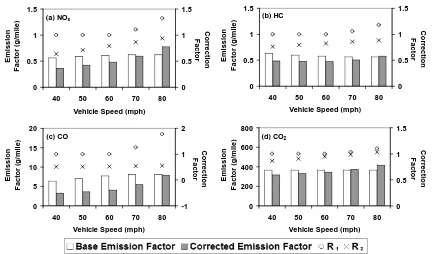
3.3.3 Case Study with High Speed and Constant Speed Correction Factors

The application of the correction factors for high speed and constant speed are illustrated based on an example case study. The case study is based on ambient conditions of 75 °F, 50% relative humidity, and 30 inches Hg barometric pressure. The results of the case study are shown in Figure 3-6 for vehicle speeds varying from 40 mph to 80 mph. The base emission rate from MOBILE6 is shown in the figure. MOBILE6 does not predict any change in the emission rate as average speed increases above 65 mph. Therefore, the base emission rates shown for speeds of 70 and 80 mph are the same for each pollutant.

(61)

the most sensitive to higher speed for CO. For example, R1 for CO is approximately 1.8 at 80 mph. R1 is the least sensitive for CO2, which is also highly correlated with the rate of fuel consumption.

The values of R2 are shown for all speeds and illustrate the ratio of the average emission rate at constant speed versus the average emission rate for transient speeds typically of driving cycles with the same average speed. Except for CO, R2 is typically the smallest at the lowest average speed shown at 40 mph, and approaches a value of 1 as speed increases to 80 mph. For CO, driving at constant speed would eliminate episodes of fuel enrichment that produce very high emissions; thus, R2 is less sensitive to average speed than for other pollutants, and generally remains approximately constant.

The combined effect of the base emission rate, R1, and R2 is shown in the corrected emission factor. The corrected emission factor represents an estimate of the emission rate at constant speed for the indicated speed. The effect of R2 on the corrected emission factor is significant for speeds of 40 to 60 mph. At 70 mph, the two correction factors almost compensate for each other. However, at 80 mph, the high speed correction factor has a more significant effect on the corrected emission factor than the constant speed correction factor.

(62)

For CO, the constant speed correction factor is the dominant influence on the corrected emission factor for speeds of 40 to 70 mph. At 80 mph, the two correction factors approximately compensate for each other.

For CO2 emission rate, which is indicative of fuel consumption, the corrected emission factor is approximately 14 percent lower at 40 mph and 13 percent higher at 80 mph. R2 is a more significant influence at lower speed, whereas R1 is a more significant influence at high speed.

At high speed, the emission factors for NOx are sensitive to the high speed correction factor, whereas for HC and CO the two correction factors tend to compensate to a large extent. As expected, the CO2 emission factor is estimated to increase at 80 mph compared to lower speeds.

3.4 Conclusions

(63)

In general, emission factors for NOx, HC, and CO2 are found to be sensitive to the difference between constant versus transient speed for low speeds, with this difference decreasing on a relative basis as speed increases. In contrast, CO emissions are more sensitive to the difference between constant and transient speed at all speeds evaluated here. NOx emissions at constant speed are significantly different than for transient operations. For example, at an average speed of 40 mph, constant speed operation can reduce the NOx emission rate by 36 percent. However, as average speed increases, there is less difference in emission rate for constant versus transient speed operation. For example, at 80 mph, driving at constant speed would reduce emissions by only 6 percent. Taking into account both constant and high speed correction factors, the NOx emission rate at 80 mph is 113 percent higher than at 40 mph. Hence, the NOx emission rate is sensitive both to average speed and whether a vehicle is operated at constant or transient speeds.

The CO emission factor is highly sensitive to average speed, and increases by 125 percent when comparing transient driving at 80 mph to 40 mph. However, at all speeds considered from 30 to 80 mph, there were substantial benefits to operating a vehicle at constant rather than transient speeds, leading to reductions in emission rate of approximately 50 percent.

(64)

reduction in total HC emissions associated with operations at constant, rather than transient, speed, ranging from 12 to 23 percent.

When estimating emission rates at high constant speed, such as 80 mph, the key findings are that the NOx and CO2 emission rates were most sensitive to the combined effect of the high speed and constant speed correction factors. The corrected emission factors for these two pollutants were 24 and 13 percent higher, respectively, than base emission factors estimated using MOBILE6. For CO and HC, the two correction factors compensate for each other at 80 mph, leading to differences of only 2 percent for both.

At moderate speeds, the emission factors for all four pollutants were sensitive to corrections for constant versus transient speeds. For example, at a constant speed of 40 mph, the estimated emission factors for NOx, HC, CO, and CO2 were lower by 36, 23, 49, and 14 percent, respectively, than for transient operations at the same average speed.

The implications of these results is that on-road emissions, and hence near-roadway air quality and exposure, are sensitive to characteristics of vehicle operations that are not accounted for in the MOBILE6 model, including operations at constant speed, high speed, or both. The potential error from not accounting for these operating conditions on short segments of highway can be as large as 49 percent at moderate speed and 24 percent at high speed.

(65)

segments of highway for which vehicles may be driving at approximately constant speed. Such estimates are useful as part of assessment of emissions and air quality in the near vicinity of a roadway. A similar methodology should be developed and demonstrated for diesel vehicles. The methodology demonstrate here can also be applied with the modal emission factors that are the basis of the Draft MOVES 2009 model.

3.5 Acknowledgments

(66)

3.6 References

Beardsley, M., 2001. Development of Speed Correction Cycles. EPA420-R-01-042, U.S. Environmental Protection Agency, Washington, DC.

Brugge, D., Durant, J. L., Rioux, C., 2007. Near-highway pollutants in motor vehicle exhaust: A review of epidemiologic evidence of cardiac and pulmonary health risks. Environmental Health 2007(6), 23, doi:10.1186/1476-069X-6-23.

http://www.ehjournal.net/content/6/1/23 (accessed 06/25/09). Census Bueaeu, 2008. American Housing Survey.

http://www.census.gov/hhes/www/housing/ahs/ahs03/ahs03.html (accessed Feb. 20, 2008). Environmental Protection Agency, 2003. User’s Guide to MOBILE6.1 and MOBILE6.2: Mobile Source Emission Factor Model. EPA420-R-03-010, U.S. Environmental Protection Agency, Ann Arbor, MI.

Environmental Protection Agency, 2008. National Emissions Inventory (NEI) Air Pollutant Emissions Trends Data. http://www.epa.gov/ttn/chief/trends/ (accessed May 20, 2008). Environmental Protection Agency, 2009a. Integrated Science Assessment for Carbon

Monoxide (First External Review Draft). EPA600-R-09-019, U.S. Environmental Protection Agency, Research Triangle Park, NC.

Environmental Protection Agency, 2009b. Draft Motor Vehicle Emission Simulator (MOVES) 2009 User Guide. EPA-420-B-09-008, U.S. Environmental Protection Agency, Ann Arbor, MI.

Environmental Protection Agency, 2009c. Fuel Economy Guide 2009.

http://www.fueleconomy.gov/feg/FEG2009.pdf/ (accessed June 26, 2009).

Frey, H.C., Unal, A., Chen, J., Li, S., Xuan, C., 2002. Methodology for Developing Modal Emission Rates for EPA's Multi-scale Motor Vehicle & Equipment Emission System. EPA420-R-02-027, Prepared by North Carolina State University for U.S. Environmental Protection Agency, Ann Arbor, MI.

Frey, H.C., Zhang, K., Rouphail, N.M., 2008. Fuel Use and Emissions Comparisons for Alternative Routes, Time of Day, Road Grade, and Vehicles Based on In-Use Measurements. Environmental Science and Technology 42(7), 2483-2489.

(67)

Nam, E.K., 2003. Proof of Concept Investigation for the Physical Emission Rate Estimator (PERE) for MOVES. EPA420-R-03-005, U.S. Environmental Protection Agency, Ann Arbor, MI.

(68)

Table 3-1. Definition of VSP Modes for Light Duty Gasoline Vehicles.

VSP Mode VSP Range (kW/ton)

1 VSP ≤ -2

2 -2 < VSP < 0

3 0 ≤ VSP < 1

4 1 ≤ VSP < 4

5 4 ≤ VSP < 7

6 7 ≤ VSP < 10

7 10 ≤ VSP < 13

8 13 ≤ VSP < 16

9 16 ≤ VSP < 19