Fixed-width digital multipliers based on recursive architectures.

Electronic Theses and Dissertations

Theses, Dissertations, and Major Papers

1-1-2006

Fixed-width digital multipliers based on recursive architectures.

Fixed-width digital multipliers based on recursive architectures.

Kevin Biswas

University of Windsor

Follow this and additional works at:

https://scholar.uwindsor.ca/etd

Recommended Citation

Recommended Citation

Biswas, Kevin, "Fixed-width digital multipliers based on recursive architectures." (2006). Electronic Theses

and Dissertations. 7094.

https://scholar.uwindsor.ca/etd/7094

by

Kevin Biswas

A Thesis

Submitted to the Faculty o f Graduate Studies and Research

through Electrical Engineering

in Partial Fulfillment o f the Requirements for

the Degree o f Master o f Applied Science at the

University o f Windsor

Windsor, Ontario, Canada

2006

1*1

Published Heritage

Branch

Direction du

Patrimoine de I'edition

3 9 5 W ellington Street

O ttaw a ON K 1 A 0 N 4

C anad a

395, rue Wellington

Ottawa ON K1A 0N 4

Canada

Your file Votre reference

ISBN: 978-0-494-35955-6

Our file

Notre reference

ISBN: 978-0-494-35955-6

NOTICE:

The author has granted a non­

exclusive license allowing Library

and Archives Canada to reproduce,

publish, archive, preserve, conserve,

communicate to the public by

telecommunication or on the Internet,

loan, distribute and sell theses

worldwide, for commercial or non­

commercial purposes, in microform,

paper, electronic and/or any other

formats.

AVIS:

L'auteur a accorde une licence non exclusive

permettant a la Bibliotheque et Archives

Canada de reproduire, publier, archiver,

sauvegarder, conserver, transmettre au public

par telecommunication ou par I'lnternet, preter,

distribuer et vendre des theses partout dans

le monde, a des fins commerciales ou autres,

sur support microforme, papier, electronique

et/ou autres formats.

The author retains copyright

ownership and moral rights in

this thesis. Neither the thesis

nor substantial extracts from it

may be printed or otherwise

reproduced without the author's

permission.

L'auteur conserve la propriete du droit d'auteur

et des droits moraux qui protege cette these.

Ni la these ni des extraits substantiels de

celle-ci ne doivent etre imprimes ou autrement

reproduits sans son autorisation.

In compliance with the Canadian

Privacy Act some supporting

forms may have been removed

from this thesis.

While these forms may be included

in the document page count,

their removal does not represent

any loss of content from the

Conformement a la loi canadienne

sur la protection de la vie privee,

quelques formulaires secondaires

ont ete enleves de cette these.

Signal processing applications, in general, require a constant word size throughout

the processing system. This poses a problem for basic integer arithmetic operations,

where the result o f each operation has a tendency o f differing from the original operand

size. Multiplication is o f the biggest concern since each operation results in a product

that is potentially twice as large as the original operand widths. To alleviate the problem

o f expanding word widths, fixed-width multipliers are utilized.

This thesis will present some novel architectures for fixed-width recursive

multipliers. The high-performance recursive multiplier exhibits an inherent hierarchical

structure consisting o f several sub-multipliers, which makes it suitable for fixed-width

applications.

Four truncation schemes targeting the recursive multiplier have been

proposed, all o f which improve error statistics and generally reduce gate complexity,

propagation delay, and power consumption, with respect to the original full-width

multiplier. A fixed-width architecture targeting multi-level recursive multipliers will also

The work presented in this thesis would not have been possible without the

support from my colleagues, mentors and family. I am deeply indebted to all of them.

Firstly, I would like to express my sincere gratitude and appreciation to my

supervisor Dr. M ajid Ahmadi for his generous support and guidance. He has made, and

will continue to make, tremendous impact on me academically, socially and personally,

through his endless enthusiasm towards my work and excellent advice in all o f my

endeavours.

I would like to thank the faculty at the University o f Windsor, including my

internal reader, Dr. Huapeng Wu, and Dr. Maher Sid-Ahmed for their advice, guidance

and words o f inspiration. I would also like to thank my external reader, Dr. Arunita

Jaekel for her patience and support.

To Mr. Ashkan Hosseinzadeh Namin and Mr. Pedram Mokrian I also extend my

sincere gratitude and appreciation, not only for their sound technical advice, but for their

great friendship.

Finally to my parents, Olive and Nihar, my brother, Robert, and Nichole Jun, I

must extend my most sincere love and gratitude, for their unending support, patience and

A B STR A C T

...iii

D E D IC A TIO N

... iv

ACKNOW LEDGEM ENTS...v

L IST O F TA B LE S... viii

L IST O F FIG U RES...ix

CHAPTER

1. INTRODUCTION TO COMPUTER ARITHMETIC

1.1 Overview o f Computer A rithm etic... 1

1.2 Thesis H ighlights... 1

1.3 Thesis Organization...2

2. DIGITAL MULTIPLICATION OVERVIEW

2.1 Basics o f Digital Multiplication... 5

2.2 Sequential Multiplication... 6

2.3 Parallel M ultiplication... 8

2.4 Floating Point Number System and M ultiplication... 12

3. FIXED-WIDTH MULTIPLICATION

3.1 Overview o f Fixed-Width M ultiplication...15

3.2 Truncated M ultipliers...16

3.3 Truncation Schemes for Fixed-W idth M ultipliers...18

4. THE RECURSIVE MULTIPLIER

4.1 Overview o f the Recursive M ultiplication Algorithm ...25

4.2 Recursive Multiplication A rchitecture...27

5. FIXED-WIDTH RECURSIVE MULTIPLIER ARCHITECTURES

5.1 Proposed Truncation Schemes for Recursive M ultipliers... 31

5.2 Error Simulation and Analysis... 35

6.2 Simulation R esults... 44

7. FIXED-WIDTH MULTI-LEVEL RECURSIVE MULTIPLIERS

7.1 Multi-Level Recursive M ultiplication...46

7.2 Proposed Truncation Scheme for Multi-Level Recursive

M ultipliers... 47

7.3 Error Simulation and Complexity A nalysis... 48

8. CONCLUSIONS

8.1 Summary o f C ontributions...53

8.2 Concluding R em arks... 54

REFEREN CES...55

APPENDICES

Appendix A: C Code for Error Simulation Program s...58

Appendix B: Verilog HDL C ode... 68

Appendix C: Simulation Reports and Logs from Altera Quartus I I ...82

Table 3.1: Error Statistics for Constant Correction M ultipliers...20

Table 3.2: Complexity Savings From Truncation o f Array and Dadda M ultipliers

21

Table 5.1: Error Statistics for Proposed Fixed-Width Recursive M ultipliers...36

Table 5.2: Error Statistics for Different Fixed-Width M ultipliers... 37

Table 5.3: Complexity Savings Comparison o f Each Scheme (2

n

= 8 ) ... 40

Table 5.4: Complexity Savings Comparison for Larger M ultipliers (2

n

=16, 32,64).... 40

Table 5.5: Overall Performance Comparison o f Proposed Truncation Schem es... 41

Table 6.1: FPGA Simulation Results... 44

Table 7.1: Error Simulation Results for Fixed-Width Two-Level Recursive Multipliers49

Table 7.2: Maximum Positive Error for Different Levels o f Recursion... 51

Figure 2.1: Example o f Pen and Paper M ultiplication... 5

Figure 2.2: Partial Product Array for a 16-bit M ultiplication...6

Figure 2.3: Sequential Right-Shift M ultiplier... 7

Figure 2.4: Multiplication Performed Using Radix-4... 8

Figure 2.5: Standard Layout o f an Array M ultiplier...9

Figure 2.6: Flow Diagram o f a Column Compression M ultiplier...10

Figure 2.7: Dot Diagrams o f Dadda and Wallace M ultipliers... 11

Figure 2.8: IEEE Floating Point Standard Word W id th s... 13

Figure 2.9: A Floating Point Multiplication Scheme...13

Figure 3.1: Standard and Truncated Array M ultipliers... 17

Figure 3.2: Standard and Truncated Tree (Dadda) M ultipliers... 17

Figure 3.3: Truncated Partial Products Matrix with Constant Correction... 19

Figure 3.4: Truncated Partial Products Matrix with Data-Dependent Correction... 22

Figure 4.1: Block Diagram o f Recursive Multiplier A rchitecture... 27

Figure 4.2: Another Block Diagram o f Recursive Multiplier A rchitecture...27

Figure 4.3: Full Dot Diagram o f a Recursive Multiplier with «-bit Onput O perands

28

Figure 4.4: Delay Comparison o f Array, Dadda and Recursive M ultipliers...29

Figure 5.1: Fixed-W idth Recursive M ultiplier... 32

Figure 5.2: Proposal # 1 ... 33

Figure 5.3: Proposal # 2 ... 34

Figure 6.1: RTL Schematic Diagram o f a "32-bit Fixed-W idth Recursive Multiplier

Using Proposal #4 (16 correction bits)"... 43

Figure 7.1: Graphical Representation o f Truncation in a Two-Level Recursive

M ultiplier... 48

Figure 7.2: Graphical Representation o f Complexity Savings for

k ~

1,2, and 3 ...52

CHAPTER 1

INTRODUCTION TO COMPUTER ARITHMETIC

1.1 Overview of Computer Arithmetic

The computer has permeated our professional and private lives by simplifying

tasks which were once difficult or even impossible to carry out. Computers have a long

history, dating back several centuries, when mathematicians and scientists first developed

machines to help them manipulate and compute numbers [1]. The field o f computer

arithmetic was established at the birth o f these electronic computing machines. Today

the field is a sub-set o f computer architecture and deals with the implementation of

arithmetic algorithms in hardware and software for processor architectures and, more

specifically, arithmetic logic units (ALU). This thesis deals with the multiplication

architectures, which are critical components o f ALUs and other systems which perform

numerical processing. Specifically, multiplication in fixed-width applications will be

studied.

1.2 Thesis Highlights

This thesis will present a general investigation o f fixed-width multiplication and

truncation schemes, and will describe some novel architectures for fixed-width recursive

multipliers [2], The recursive multiplier, presented by Swartzlander et al. [3] exhibits an

inherent hierarchical structure consisting o f several sub-multipliers, which makes it

suitable for fixed-width applications. Four truncation schemes targeting the recursive

gate complexity, propagation delay, and power consumption with respect to the full-

width multiplier. Detailed error analysis and architectural complexity analysis have been

carried out for each design.

Hardware implementation o f the proposed fixed-width multiplier architectures has

been carried out in Altera Stratix EP1S10F484C5 FPGA. The resulting reductions in

propagation delay, power consumption and logic complexity with respect to the full-

width recursive multiplier have been tabulated and analyzed.

Further, the idea of fixed-width multipliers based on

multi-level

recursive

architectures has been studied in detail. The previous work regarding fixed-width single-

level recursive multiplication has been extended to the multi-level case, and error

analysis and complexity analysis have been carried out. N ew mathematical expressions

have been derived to estimate potential maximum error and complexity savings for the

general case o f

k

levels o f recursion.

1.3 Thesis Organization

The thesis will begin with a general overview o f digital multiplication, briefly

highlighting serial and parallel multiplication algorithms, in Chapter 2. Chapter 3 will

give an overview o f fixed-width multiplication and truncated multipliers. Further, some

o f the most well-known truncation schemes available will be described.

Chapter 4 is dedicated to the Recursive Multiplier. A n overview o f the recursive

or “divide and conquer” algorithm for multiplication proposed by Karatsuba and Ofman

(1962) [4] will be first given. Application o f the algorithm in the digital recursive

Chapter 5 will present novel architectures for fixed-width recursive multipliers.

Four new truncation schemes targeting recursive multipliers will be presented in this

chapter along with detailed error and complexity analysis. Chapter 6 will focus on

hardware implementation and simulation results o f proposed architectures. Chapter 7

investigates fixed-width multiplication using multi-level recursive architectures.

The

thesis will conclude with a highlight o f contributions and some closing remarks in

CHAPTER 2

DIGITAL MULTIPLICATION OVERVIEW

In modem digital systems, the component responsible for handling arithmetic

operations is the Arithmetic Logic Unit (ALU). These units mainly lie in the critical data

path o f the core data processing system elements. These include microprocessors (CPU),

digital signal processors (DSP), in addition to application specific (ASIC) and

programmable (FPGA) processing and addressing integrated circuits. Performance o f a

system, in regards to numerical applications, is directly related to the structure and design

o f the ALU.

The numerical operations carried out by the arithmetic unit may include, but are

not limited to: addition/subtraction, shift/extension, comparison, increment/decrement,

complement, trigonometric functions, multiplication, division, square root extraction,

logarithmic function, exponential function and hyperbolic functions [5].

One o f the critical functions carried out by the ALU is multiplication. Although it

is not the most fundamentally complex operation, digital multiplication is one o f the most

frequently used operations in signal processing and other applications. Because o f this,

digital multiplication is one o f the most widely studied areas in the field o f computer

2.1 Basics of Digital Multiplication

Generally speaking, digital multiplication involves a sequence o f additions carried

out on partial products. The means by which the partial products matrix is summed is the

key distinguishing factor amongst multiplication schemes [6].

The partial product array o f an

M

x

N

bit digital multiplication is determined

similarly to traditional pen and paper decimal multiplication. For example, multiplication

o f multiplier

X =

x„_2,

x„_3, ...

x2, x h x 0]

and multiplicand

A = [am_uam_2, a

m_3, ...

a2, ah

u„]

yields the final product

(n+m)-b\\

product:

P ~

P n

P n m -h ■■■ Pt> P b P<)\ ~~

d m_

d m.3,

d 2,

Cl/, Cl())

X„_2(Clm_\, Clm.2, Clm.3,

Ct2, Cl), Clo)

X ) ( d m.\, d m.

d m.3,

d 2, d ) , d 0)

X o ( d

d m.

d m_3,

d 2, d ) , d o )

This multiplication can be illustrated in Figure 2.1, below.

a s

a t

a g

x i

x 2

x i

x o

XgOs

X g flt

X f f i t

XgOg

X g fts

x 0a 2

x Sa l

x Ca 0

XgOs

XgOy

X g flj

XgOg

x 0°3

x 0a 2

x 0a l

x 0 °0

P ?

P i

P S

P 4

P i

P 2

P i

PO

Figure 2.1: Example o f Pen and Paper M ultiplication

A convenient notation for digital multiplication that visually represents the bits in

an algorithm is dot notation which was introduced in [7] [8].

The nature of the dot

in which they are manipulated, irregardless o f the value o f each bit. Figure 2.2 shows the

partial product array for a 16x16 multiplication [7].

ut

+

V

Product

Figure 2.2: Partial Product Array for a 16-bit M ultiplication [7]

2.2 Sequential Multiplication

Fundamentally, digital multiplication can be carried out through a sequence o f

shifts and additions o f the

multiplicand

to the partial product accumulator register based

on the values o f the individual bits comprising the

multiplier.

This primitive form o f

multiplication, known as shift-add multiplication, is very slow, despite having a very

simple implementation. The number o f cycles required to perform a full multiplication is

linearly proportional with the size o f the multiplier, and each cycle has a delay o f the

/ k

\ M U X

V"

M u ltip lic a n d M u ltip lie r P a r ti a l P r o d u c t s

Figure 2.3: Sequential Right-Shift M ultiplier [6]

A variation o f the basic form o f digital multiplication is the high-radix

multiplication scheme. This form is similar to the shift-add algorithm mentioned before,

but differs in that more than one bit o f the multiplier is utilized on each clock cycle. Thus

the number o f clock cycles is reduced.

However, a requirement for this form o f

multiplication is the availability o f fixed multiples o f the multiplicand [5]. Figure 2.4

depicts the implementation o f a radix-4 multiplier where two bits o f the multiplier are

used in a clock cycle [6]. As can be seen, the multiples o f the multiplicand, A, 2A, and

3 A, need to be available. Thus the higher the radix o f a multiplier, the more stored values

will be required. Higher radix multipliers provide faster computation; but this is at the

expense o f additional hardware overhead consisting o f shift circuitry and storage registers

Partial Products

\ M U X

3A

OA 1A| 2A| (

_i

2-bit shifts

Multiplier

\ /

k-bit Adder

Figure 2.4: Multiplication Performed Using Radix-4

2.3 Parallel Multiplication

As mentioned above, serial multiplication and the concept o f shift and add

algorithms is a primitive form o f multiplication techniques which offers simple

implementation, but lacks the performance o f parallel multipliers. Most modem high-

performance systems require faster algorithms for multiplication to reduce computation

latency as much as possible.

There are two distinct categories of parallel multipliers, namely, linear parallel

multipliers, and column compression multipliers (tree multipliers). The distinguishing

characteristic o f parallel multipliers is that partial products are generated simultaneously,

and can actually be considered a special case o f high-radix multiplication, where the

highest possible radix is used, i.e. radix-2i [6]. As well, parallel multipliers limit latency

associated with carry propagation to one final fast adder.

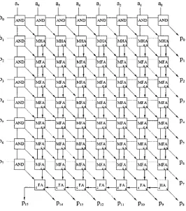
Linear parallel multipliers are more commonly known as array multipliers. The

term “linear” comes from the linear relationship that exists between operand size and

latency. The array multiplier exhibits a highly regular layout as shown in the 8-bit

design ideal for automated layout techniques, where bits o f the two input operands are

made available across the arrangement o f full adder cells. Basically the outputs o f the

adders trickle accordingly across the array until the edges o f the structure, where the

product bits are outputted. However, the limitation with the array scheme is that partial

products are introduced and reduced only one row at a time, not in parallel like in tree

multipliers. This results in slower performance. The delay o f the array multiplier has a

linear relationship, O(k), with respect to operand size.

a,

a6

a5

a4

a,

a;

a,

ao

A N D

MH.d

M F A M FA

FA H A

A N D A N D

M F A A N D

M FA

F A A N D

M FA

M FA

A N D

M FA A N D

A N D A N D

M FA M FA

M F A M FA

M F A M FA

M FA M F A

M F A

M F A

FA

M F A

M FA M FA M FA M F A

A N D

A ND

A N D M FA M F A

M FA M F A

FA F A

M F A M H A

M FA A N D

t>5 —r

M F A

M FA A N D

F A M F A

M F A

P i 5 P l4 P 13 P l2 P l l PlO P 9 P s

Figure 2.5: Standard Layout o f an Array M ultiplier

(M FA = full adder + AND gate, MHA = half adder + AND gate)

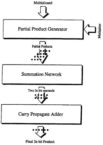
The tree multiplier, unlike the array multiplier, offers the potential for only a

logarithmic increase in delay relative to operand size.

The foundation for these

Dadda, and Yu Ofman [10][[11]. In these designs, once bits o f the partial product array

are generated (in parallel), they are passed onto a reduction network, which performs

column-wise compression of the bits, forming two final partial products. Subsequently, a

final fast adder is used to sum these last two terms. A flow diagram o f the column

compression multiplication process is shown in Figure 2.6 [7], Latency approximation of

a column compression multiplier shows that delay is logarithmic 0(log(A)) with operand

size, a significant improvement over array multipliers, in terms o f speed.

Multiplicand

Partial Products

Two 2n bit operands

Partial Product Generator

Carry Propagate Adder

Summation Network

Final 2n bit Product

Figure 2.6: Flow Diagram o f a Column Com pression M ultiplier

Wallace [10] initially proposed the method o f using Carry-Save Adder (CSA)

arrays to carry out the column-wise compression o f the partial product bits.

Consisting

o f a series o f non-interlinked Full-Adder blocks, CSA is the most commonly used form

the CSA column compression tree so that the minimum number o f counters is utilized

[11]. Wallace and Dadda multiplication schemes are depicted in Figure 2.7.

Despite the characteristic high speed performance o f column compression

multipliers, there are several drawbacks when taking into consideration their

implementation. Column compression multipliers exhibit a highly irregular architecture

leading to inefficient VLSI layout.

As process technologies delve into submicron

dimensions, irregular interconnections can potentially cause issues like clock skewing

and interconnect delay [12].

Column 22 21 20 19 18 17 16 15 14 13 12 11 10 9 8 7 6 5 4 3 2 1 0 Column 2221 20 1918 17 16 15 14 13 1211 10 9 8 7 6 5 4 3 2 1 0

Stage L

(3.2): 8 (2.2): 4

Stage 2 (3.2): 27 (2.2): 3

Stage 3 (3,2): 28 (22): 2

: x ////x

: : / / / x :

: : : > x ::

/ / / / / / / / / / / / .

;

y / / / / / / / / a

:

: :

/ / / / / / / y

: :

V / / / / / / / / / / / / / / A

:

V / / / / / / / / / / / / A

:

(w>7 •

V / / / / / / / / / / / / / / / / A

:

(2,2). 1

g |»

V / / / / / / / / / / / / / / / / / / A

Y / / / / / / / / / / A

X

/// / / / / / / / X

•

X

/ / / / / / / / / / X

*

:s :r X

/ / / / / / / / / / X

. .

Y / / / / / / / / / / A

A A A / / / / / / / / / A A

'

(3.2): 2 0 ...

(2.2): 6 ...

X X //////////X X

££f A A / / / / / / / / / / A A

Stage 4 (3.2): 11

(2.2): 3 .

Y A / / / / / / / / / / / A A A

gvxx/x//x/x/x//xxxxx

2.4 Floating Point Number System and Multiplication

To achieve the levels o f precision demanded by modem systems, it becomes

necessary to have a number system that is capable o f representing real numbers. Fixed-

point systems, in which location o f the decimal point is pre-defined, suffer from limited

range and/or precision. To alleviate this issue, floating-point number systems are utilized

[5]. Unlike fixed-point representations, floating-point system allows for extremely large

or small numbers to be described with a high degree o f precision by using a dynamic

range.

According IEEE standard for binary floating-point systems [13], a floating-point

value is defined as:

x = ± f x b e

where x is the floating-point value, / is the fraction o f mantissa,

b

is the base (fixed at

b=

2) and

e

is the exponent. Floating point numbers have two distinct representations

according to the standard depending on operand size. Figure 2.8 depicts the differences

between the two floating point standards, in terms o f word structure. The sign (s),

exponent

(e),

and fraction/mantissa

(f)

form the 32 and 64 bit precision formats. The

mantissa is normalized to be in the range o f [1,2) so that the most significant bit (MSB) is

always a 1. In this way, the leading 1 is removed and considered a “hidden one”, thus

saving one bit in the representation.

To ensure a positive value, the signed integer

exponent is biased accordingly. The exponent is biased for 127 for single, and 1023 for

(a)

(b)

23

11

52

msb

Figure 2.8: IEEE Floating Point Standard W ord W idths for

(a) Single Precision and (b) Double Precision

Figure 2.9 shows a block diagram o f the multiplier implementation for floating

point numbers. As described above, floating-point numbers are composed o f a biased

non-negative integer exponent, and a fixed-point fractional representation o f the

mantissa. Thus, mathematical operations that are carried out on floating-point numbers

will use fixed-point arithmetic units with additional control and rounding circuitry to

accommodate for the dynamic range.

Because o f this, when designing arithmetic

hardware, much attention is placed on fixed-point integer units. Conversion to floating

point is made possible through additional circuitry. Figure 2.9 also shows the additional

blocks surrounding the integer multiplier component.

U n p a ck

A d d X B ias

Multiplier

A d d

\ Add

A d d

P ack X O R

R ig h t S hift

Normalize

R o u n d

Since the basics o f fixed-point arithmetic form the framework for floating point

calculations, the remainder o f this thesis will target integer arithmetic structures in

CHAPTER 3

FIXED-WIDTH MULTIPLICATION

3.1 Overview of Fixed-Width Multiplication

As previously mentioned, multiplication is one o f the most widely studied areas in

the field o f computer arithmetic, due to the frequency o f use in numerical applications,

such as signal processing. In many o f these applications, such as filtering, convolution,

Euclidean distance, and Fast Fourier Transform (FFT) [15] [23], a constant operand size is

required throughout the processing system. When designing arithmetic hardware for

such a system, constant operand size is an important constraint to take into consideration.

In certain signal processing applications, word sizes could grow significantly large. For

example in a complex FFT, if the initial word size is 16 bits real and 16 bits imaginary

and the sines/cosines are 16 bits each, maintaining full precision causes a growth o f 18

bits (17 bits for the complex multiply and 1 bit for the complex add) per stage. For a

1024 point FFT there are 10 stages producing a final data size o f 196 bits [16]. For

addition and subtraction, the problem is relatively easy to solve, as the result is

potentially only one bit larger than the operands (assuming that the operands are equal in

size). Rounding is accomplished by adding a ‘ 1 ’ to the least significant bit position and

truncating the sum at that position. In many cases the ‘ 1’ can be added as a carry into the

addition so that no extra hardware or time is required to produce a rounded sum or

difference [16]. However, o f all the arithmetic operations, multiplication is o f the biggest

concern, because the resulting product o f two operands could potentially have a word size

To alleviate the problem o f expanding word widths in multiplication, fixed-width

multipliers are utilized [17]. An

n

x

n

fixed-width digital multiplier generates only the

most significant

n

product bits with two «-bit inputs. If

X

and

Y

are two

n

-bit unsigned

numbers where,

A = f > , . - 2 '

and

Y = ^ y j -2J

1=0

j

the product,

P,

o f

X

and

Y,

which is a weighted sum o f partial products, is therefore:

n- 1 n ^ l 2 n - \

i= 0

j =

k=

The fixed-width product is:

c

= Z

r

' 2‘

k=n

Thus a fixed-width multiplier can be easily realized by using only

p

2

n-

i,

■■■, p n

outputs o f

the full-width multiplier. In order to reduce the error due to truncation, output rounding

is often carried out. Before truncation, rounding is applied [14] by adding a ‘1’ at the

nA

least significant position o f the product o f the full-width multiplier.

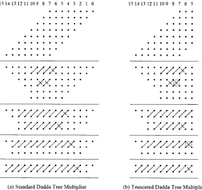
3.2 Truncated Multipliers

Literature shows that the “fixed-width” property can be exploited to reduce

hardware complexity with respect to the full-width multiplier [9]. Truncated multipliers,

in which less significant columns o f the partial product matrix are removed, are often

used in fixed-width applications. Example o f a truncated array multiplier and Dadda

b4

b,

MFA

MFA MFA MFA MFA MFA

MFA

MFA AND

P:

s.

Pi

V

P“1

P> b,

b,

b4

b,

P6

b7

P i s P m P l 3 P12 P i l Pifl P s

(a) Standard Array Multiplier

MFA

MFA

AND MFA RFA

l \ r r \

MFA AND

MFA

MFA MFA

P is P u P l 3 P12 P n P ic

(b) Tnm cated Array Multiplier

Figure 3.1: Standard and Truncated Array M ultipliers

15 14 13 12 11 10 9 8 7 6 5 4 3 2 1 0 15 14 13 12 1 1 10 9 8 7 6 5

XXXX

: x x :

xxxx

•: xxxxxxxx x x

: xxxxxx

x * •

• xxxxxxxxxx :: *

• • « • • • • • * • • •

xxxxxxxxxxxx: ■

*: xxxxxxx

: xxxxx:

• xxxxxxxx

xxxxxxxxx

(a ) S tand ard D a d d a T re e M u ltip lie r (b ) T ru n ca ted D a d d a T re e M u ltip lie r

3.3 Truncation Schemes for Fixed-Width Multipliers

Several truncation schemes have been developed— all o f which involve not

generating the complete partial products matrix and then applying some correction

scheme to reduce the error due to truncation as well as post-rounding. This subsection

examines some o f the schemes which currently exist for parallel multipliers.

Constant Correction Truncation Scheme

In [18], Schulte and Swartzlander, Jr. presents a technique for parallel

multiplication which computes the product o f two numbers by summing only the most

significant columns o f the multiplication matrix, along with a correction constant. This

correction constant is chosen such that average and mean square errors, with respect to

the full-width multiplication, are minimized.

In the conventional parallel full-width multiplier,

n2

partial product bits are

summed to produce the final 2

n

bit product. As mentioned before, the fixed-width

multiplier is formed by rounding the 2

n

result to

n

bits.

Substantial hardware savings can be achieved by truncated multiplication, where

only the

n+k

most significant columns o f the partial products matrix are summed.

Truncated multiplication involves two sources o f error, namely, reduction error and

rounding error.

Reduction error results from summing the partial products matrix

without the

n-k

least significant columns. Rounding error occurs because the product is

rounded to

n

bits. To compensate for these two sources o f errors, a correction constant is

added to the

n+k

most significant columns o f the partial products matrix, as shown in

presented in [19]. In this paper reduction error and rounding error are treated separately,

resulting in a poorly selected correction constant. Also, the constant is allowed to take on

arbitrary values, which is unfavourable for practical implementations. The correction

constant should be limited to the

n+k

most significant columns.

Ca-1 * - - - ...- Cu-k -l C u-k

^n-k+l^\) ^n-k ^3

an-ibi... (Vt bi Ak-ib

i

. a i b o k a 0b il k

. - ' a 0b n - M

K X i

A ’bn-2

-... --■■■■... 81 ba-2

r

A -

i

anA-i... a A i f'ohi-i

f t a - 1 f t a - 2 f t * 3 --- R . f t - 1 ---P U - 1 f t - k

Figure 3.3: Truncated Partial Products M atrix with Constant Correction

The value o f the computed product can be expressed in the following way:

P ' = P + F

+ F

+ C

where

P

is the true product,

Ereduct

and

Eround

are the reduction and rounding errors, and C

is the correction constant. To minimize the average error o f the truncated multiplication,

or

P ’-P,

the correction constant is selected to be as close as possible to the negative o f the

expected value o f the sum o f the reduction error and the rounding error. Assuming that

the probability o f any input bit,

a,

or

bj,

being a one is 0.5, and a partial product bit, 0.25,

the following formula can be used in determining the correction constant, C [18]:

round(2n+k ■ Etotal)

2n+k

where

E „ ,

= - ^ " s ' («■ + D •

- (1 - 2~‘ )

Using exhaustive simulation, error statistics have been determined for multipliers o f size

n

= 8, and 16 bits. Average error, variance and maximum error have been tabulated, as

shown in Table 3.1. As can be seen, as

k

decreases, errors generally tend to increase.

Table 3.1: Error Statistics for Constant Correction M ultipliers

n

A

Eave

Variance

t-max

17

8

1

-9.766 x iff4

0.1667

2.5039

2

6.152 x 10"2

0.1040

1.2539

3

6.152 x 10'2

0.0903

0.7539

4

-1.660 x 1 O'2

0.0842

0.6289

5

-9.766 x 1 O'4

0.0834

0.5352

8

1.953 x 10‘J

0.0833

0.5000

16? ;

1

-3.815 x 10'b

0.2917

5.5000

2

6.250 x 10‘2

0.1354

2.7500

3

6.250 x 1 O'2

0.0983

1.5000

4

-1.563 x lO"4

0.0861

1.0000

5

-3.815 x 10'6

0.0839

0.7188

16

7.629 x 1 O'6

0.0833

0.5000

As described earlier, parallel multipliers are usually implemented as array or tree

(column compression) multipliers. Conventional

n

x

n

multipliers require

n2

AND gates,

n - 2n

full adders and n half adders. If the least significant

t

=

n-k

columns are omitted

from computation then hardware savings can be approximated as [18]:

AND gates, ——

—— Full adders, ( t- 1 ) H alf adders.

A typical

n

x

n

bit Dadda multiplier requires

n2

AND gates,

n2-4n+3

full adders and

n

- 1

half adders (for

ri>

2).

Similarly the hardware saved with a truncated Dadda multiplier

(f>l) is [18]:

AND gates,

Full add

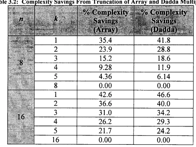
The following table (Table 3.2), taken from [18], shows hardware savings for various

sizes o f truncated multipliers with respect to a conventional multiplier utilizing true

rounding. This data is calculated based on the assumption that relatives sizes o f AND

gates, half adders and full adders are 1, 4 and 9, respectively. Complexity savings are

slightly higher for Dadda multipliers. As expected, a small value o f

k

results in larger

complexity savings.

Table 3.2: Com olcvity Savings From Truncation o f Array and Dadda M ultipliers

71

i*£ - -V

* - r.

* t '*<•

% Complexity

Savings

(Array)

% Complexity

Savings

(Dadda)

P

V

W

W

M

H

1

35.4

41.8

2

23.9

28.8

3

15.2

18.6

4

9.28

11.9

5

4.36

6.14

8

0.00

0.00

16

1

42.6

46.6

2

36.6

40.0

3

31.0

34.2

4

26.2

29.3

5

21.7

24.2

16

0.00

0.00

Data-Dependent (Variable) Correction Truncation Scheme

In the constant correction method for truncated multiplication, the correction term

does not depend on the values o f the bits in the truncated portion o f the partial products

matrix. Potentially, this could lead to relatively high errors, in the case that the all or the

majority o f truncated bits are a zero or a one.

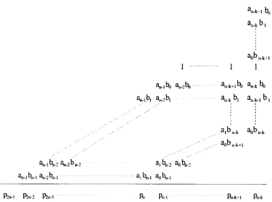
In [20], King and Swartzlander, Jr. presents a correction method that uses the

This results in a variable correction term, which can further minimize distortion to the

result.

In the method o f constant correction, the maximum error occurs when truncated

bits (columns

n+k

+ 1 and beyond) are all zeros or all ones. If the truncated bits are all

zeros, then the final error with respect to the full-width multiplier would be equal to the

correction value. In this case, ideally, the correction value should be set to zero. If the

n+k+l

column contains the same number o f ones as zeros, then the constant proposed in

by Schulte and Swartzlander in [18] should be used. Finally, if the

n+k+l

column

contains all ones, the correction value should be changed to a maximum value. King and

Swartzlander use the number o f partial products available in the

n+k+l

column. The

correction term is simply added as a “Carry-in” to the

n+k

column, as shown in Figure

3.4.

a „ . k - i h ,

a o i , n -k » l

1

1

1

a»A a„A

a ^ A

bn

a.-i.b, a^b,

a,,.t b, a ^ b ,

. a,bu.k Etobjj.,.

.

- a0b„.^,

a» A : a^b..,

a, b,.: a A :

Vibi.! a,,A-i

a,^,., aA.i

P ’n -l p 2 n -2 P211-.I P u Pn-1 R i-k + l R i-k

Figure 3.4: Truncated Partial Products Matrix with Data-Dependent Correction

Results show that mean error, maximum error and variance are improved with

array multipliers, while constant correction schemes are more suitable for tree multipliers

[9]-Other Truncation Schemes

Since the work o f Swartzlander, Lim, Schulte, and King in the late 1990s, there

have been several new schemes, fundamentally based on the concepts o f constant and

variable correction, presented in literature.

A correction algorithm is developed in [21] by Jou et al. where the partial

products in the most significant column o f the truncated portion o f the matrix are

summed together. From this sum, a correction constant is calculated that approximates

the sum o f the dropped partial products. The method improves error over traditional

constant correction, however the implementation is based on a ripple architecture that is

slow in speed and consumes much power [15].

In [22], Van et al. propose a fixed-width multiplier architecture that is similar to

the constant correction method, where a constant is added to the remaining partial

products matrix after truncation. The correction factor, however, is not based on the sum

o f the most significant column o f the truncated portion, but rather is a function o f the

single partial products o f the subset.

Only signed multipliers are considered.

Implementation o f the error-compensation function is based on ripple architecture as

well.

In [15] Strollo et al. presents a new error-compensation network for fixed-width

multipliers, consisting o f two summation trees which are optimally chosen in order to

better accuracy with respect to previous methods, and implementation o f the error

correction network requires only a few gates with a tree architecture, and thus is best

suited for tree multipliers.

Literature shows that many truncation schemes have been proposed that generally

target only array and tree multipliers. The next chapters o f this thesis are dedicated to the

recursive multiplier, originally presented by Danysh and Swartzlander [3], It will be

shown that this multiplier’s hierarchical composition makes it very suitable for fixed-

width applications. The concepts o f truncation schemes described in this chapter will be

extended to this multiplier design, resulting in four novel fixed-width multiplier

CHAPTER 4

THE RECURSIVE MULTIPLIER

4.1 Overview of the Recursive Multiplication Algorithm

One o f the pioneering schemes for “divide and conquer” multiplication was

proposed by Karatsuba and Ofman in 1962 [4]. The Karatsuba-Ofman Algorithm (KOA)

computes the multiplication o f two long integers by executing multiplications and

additions on their divided parts.

It is possible to perform multiplication o f large numbers in significantly fewer

operations than the usual brute-force technique o f long multiplication. As discovered by

Karatsuba and Ofman, multiplication o f two «-digit numbers can be done with a bit

complexity (number o f single operations o f addition, subtraction and multiplication) o f

less than

n2.

The algorithm can be illustrated with the following example [24], using two

base

X

numbers,

Ni

and

N 2,

each consisting o f two digits:

N x - a 0 + axX

N 2 = bQ+bxX

Their product can thus be written as:

p

=

n x

-

n

2

=

a0b0 +

(

a0bx + axb0) X + axbxX 2

= p 0 + p xX + p 2X 2

Now let:

qQ = aQb0

The term

q\

can then be written in terms o f

po,p\,

an d

p 2:

< h = P i + P o + P 2

But, since

po

=

qo

and

p 2 = q2,

it follows that:

Po=<lo

A = 0 1 -0 0 - 0 2

Pi ~~

Thus the three digits o f

p

have been evaluated using three multiplications rather than

four.

When the concept is extended to multi-digit numbers, the trade-off o f more

additions and subtractions becomes evident.

Danysh and Swartzlander have utilized the fundamentals o f KOA in their digital

recursive multiplication algorithm presented in [3].

Mathematically, the recursive

algorithm is established around the fact that any 2

n

x 2

n

bit multiplication may be carried

out through four

n

x

n

bit sub-multiplications. Consider two unsigned 2/r-bit operands,

the multiplicand

A = A

h

x 2" +

A

l

and multiplier

X

=

X u

x 2" +

X L,

where the

subscripts denote the lower and upper

n

bits respectively. The multiplication o f

A

by

X

may then be given by:

Y = A - X

= K » 2

" +A

l

) - {

x h x

T + X l )

= A „ - X „

2 1" + ( J

- X

+ A

- X , )

2 ’ + A

- X 1.

Multiplication and addition are thus carried out on the divided components of

A

and

X,

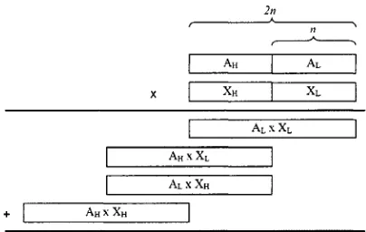
4.2 Recursive Multiplication Architecture

Block diagrams illustrating the same recursive multiplier architecture are shown

in Figures 4.1 and 4.2.

2n

•--- ‘-;

---____

| Ah j Al |

X | X H 1 X L |

| Al xXl |

|

A

h

x X

l

|

| A l x XH |

+ Ah x Xh

Figure 4.1: Block Diagram o f Recursive M ultiplier Architecture

I n

Aff x XL

A

h

x

X

h

A

l

X

XL

A

l

x X H

+

Figure 4.2: Another Block Diagram o f Recursive M ultiplier Architecture

As can be seen, the overall multiplication may be reduced to four smaller

multiplications, and this process may be repeated using even smaller multipliers for the

base multipliers. To minimize the resulting reduction delay introduced by subdividing

and parallelizing the process, the intermediary products o f the sub-multipliers should be

yield the final product. A dot diagram, for a typical recursive multiplier with «-bit

operands is shown in Figure 4.3.

n-bit multiplier

input operands

4 intermediary

n-bit products in

carry save form

i i

i 4 * 4 1 1 4

HALF-ADDER

J

Reduction Cells

I

V

_'

i

i

■

t <

'

’ r T 1

• 4 i >

11 ’

; H i ;

Final Carry-Out T

is omitted

2n-l

lti/2 -1

I

nf

2

Figure 4.3: Full Dot Diagram o f a Recursive M ultiplier with n-bit Onput Operands [5]

There are two significant benefits in using the recursive multiplier [3]. Firstly,

use o f the recursive multiplier allows for a highly regular design and scalability similar to

traditional array and modified Booth multipliers. Secondly, unlike array and modified

Booth multipliers, the recursive multiplier can achieve a delay o f 0 (lo g

n)

similar to fast

multipliers such as Dadda and Wallace. Traditional array and modified Booth multipliers

are capable o f only O

(n)

delay.

Figure 4.4 shows a graph illustrating this delay

comparison. The delays for a typical array multiplier, Dadda multiplier and recursive

multiplier may be estimated with the following expressions [3]:

^Anay = 1+ 3 (« -1 ) + 41og2(/I-1 )

Ajadda =1 + 3(2 log2

(n

-1 )) + 3 log2 (« + 1)

600

— D adda

— Recursive

500

400

a 300

200

100

-80

100

120

140

160

180

Multiplier Size (bits)

Figure 4.4: Delay Comparison of Array, Dadda and Recursive M ultipliers

Essentially, the recursive multiplier reaps the benefits o f both worlds:

the

regularity and scalability o f array and Booth multipliers, and the fast performance of

Dadda and Wallace tree multipliers. Even with the use o f array multipliers as the base

multiplier in the recursive hierarchy, a delay o f 0 (log

n)

is achieved. Use o f a faster

multiplier as the base case can slightly improve performance at the expense o f additional

complexity and irregularity.

P. Mokrian et al. presented a reconfigurable recursive multiplier architecture that

actually outperformed the typical high-performance Booth-recorded Wallace Tree

multiplier in terms o f delay (17% reduction), dynamic power consumption (20%

reduction) and area utilization (12% increase) [5].

The recursive multiplier provides a simple alternative to traditional Booth and

array multipliers with speed that is comparable or even faster than Wallace and Dadda

times. The multiplier is also scalable to higher bit precisions by simply duplicating sub­

multipliers and adding additional levels o f reduction. A negative aspect o f the recursive

multiplier is its difficulty in handling 2 ’s complement numbers. However, since we are

interested in floating point implementations consisting o f fixed-point unsigned integer

multipliers, this disadvantage o f the recursive multiplier need not be an issue in this

study.

After examining the benefits o f the recursive multiplier, it was found that the very

regular composition o f the architecture allows it to be readily applied in systems

requiring fixed-width processing.

As described before, literature shows that many

truncation schemes are available for array and tree multipliers, but none specifically for

multipliers based on a recursive architecture. The ensuing chapters will present new

truncation schemes that target the recursive multiplier. The standard array multiplier will

be used as the base multiplier in all designs, which allows for more convenient

CHAPTER 5

FIXED-WIDTH RECURSIVE MULTIPLIER ARCHITECTURES

The preceding chapter provided an overview o f the recursive multiplication

algorithm (KOA), as well as the architecture for digital recursive multiplication,

presented by Danysh and Swartzlander.

The recursive multiplier has an inherent

hierarchical structure that consists o f several sub-multipliers, making it very suitable for

fixed-width applications. Itwill be shown that rather than modifying the sub-multipliers’

structure, a truncation scheme can simply remove one sub-multiplier and replace it with a

data-dependent correction term.

As mentioned before, fixed-width multipliers have been mainly targeting array

and tree structures [9]. Truncation schemes usually involve omitting a certain number o f

the least significant columns o f the partial products matrix and then adding a constant or

data-dependent correction term to the truncated partial products matrix to reduce the error

due to truncation. Generally, rounding is then applied to the multiplier’s output. In this

chapter, four new truncation schemes targeting the recursive multiplier are proposed.

The associated computation error is analyzed, and a summary o f complexity savings

incurred as a result o f truncation is given as well.

5.1 Proposed Truncation Schemes for Recursive Multipliers

As described before, the overall multiplication in a single-level recursive

multiplier is reduced to four smaller sub-multiplications. The product o f the multiplicand

Y = A X

= ( Ah x T + Al ) . ( X h x T + X l )

= AH - X H x 2 2n+ ( A L . X H + AH - X L) x T + AL - X L.

Graphically, a fixed-width recursive multiplier can be represented by Figure 5.1. It is

clear that the accumulation o f four sub-products yields a

An

bit result whereas the product

(denoted as

Y)

has only 2

n

bits. In this format, it is evident that the first sub-product,

A

l

X

l

(highlighted), is o f minor significance with respect to the rounded 2

n

bit product.

The truncation schemes to be presented thus target this particular component.

2n

_ A .

r

X

)7

s

...

... -\

A

A

X

X

+

A

x X

Y

A

x X

A

x X

---

Y---2n

Figure 5.1: Fixed-Width Recursive M ultiplier [2]

In all the proposed truncation schemes, the sub-multiplier

A

l

X

l

is removed and

subsequently, a data-dependent correction term is added. In the design process o f all

schemes, it was desirable that the new correction term be relatively easy to generate and,

at the same time, maintains some partial information regarding the magnitude o f the sub­

paragraphs and illustrated in Figures 5.2-5.5. All schemes have a relatively short design

time.

In Proposal #1, we simply use

A

h

X

l

or

A

j

X

h

to replace the least significant

truncated term

A

l

X

l

-

In this fashion, some partial information regarding the magnitude of

the partial product is maintained, while no actual multiplication is carried out. The

advantage o f this scheme lies in the fact that the correction value is a significant term

already generated in the calculation, and thus no extra costs are created.

2 n

_______

K

_______

'

'

<>•'

A.

xh

A

X

|

4

A

jj

X

h

I

|

AjXff

|

Figure 5.2: Proposal #1

In Proposal #2, the average o f the two blocks,

AuXL

and

A

i

X

h

,

is placed in the

block o f

A

l

X

l

after truncation. This approach involves the addition o f four rows to the

partial product reduction tree o f the overall recursive structure, where the rows would be

A

h

X

l

/2 and

A

l

X

h

/2

in carry save format. This is simply a shifted version o f the two

previously generated sub-products, thus adding no significant complexity to the

architecture. The motivation behind this architecture is that a correction term with a high

A

r

A

l

AhXl + AlX „ 2

A

h

X

h

a l x h

Figure 5.3: Proposal #2

In Proposal #3, the most significant partial product bit, namely

an.ix„.i,

generated

by the block

A

l

X

l

,

is added at the least significant bit position o f block

A

h

X

h

. Once

again, the aim is to maintain some partial information regarding the magnitude o f the

partial product without carrying out a full multiplication. The correction bit is simply

implemented with one two-input AND gate. With a 1-bit correction term, accumulation

o f the partial products matrix is simplified, thus requiring less reduction circuitry.

A i

—

an_ian_2...ctiao

X L

=

.. .X

X

AffAf?

A

l

X

h

Figure 5.4: Proposal #3

Proposal #4 is essentially an extension o f the scheme in Proposal #3, allowing

additional correction bits to be used for further error correction. A significant difference,

however, is that the first correction bit,

an.ixn.i

is added at weight 22"'1, which is simply