On: 04 October 2012, At: 08:29 Publisher: Routledge
Informa Ltd Registered in England and Wales Registered Number: 1072954 Registered office: Mortimer House, 37-41 Mortimer Street, London W1T 3JH, UK
Annals of the Association of American Geographers
Publication details, including instructions for authors and subscription information: http://www.tandfonline.com/loi/raag20FUTURES: Multilevel Simulations of Emerging
Urban–Rural Landscape Structure Using a Stochastic
Patch-Growing Algorithm
Ross K. Meentemeyer a , Wenwu Tang a , Monica A. Dorning a , John B. Vogler a , Nik J. Cunniffe b & Douglas A. Shoemaker a
a
Department of Geography and Earth Sciences, University of North Carolina at Charlotte b
Department of Plant Sciences, University of Cambridge Version of record first published: 04 Oct 2012.
To cite this article: Ross K. Meentemeyer, Wenwu Tang, Monica A. Dorning, John B. Vogler, Nik J. Cunniffe & Douglas A. Shoemaker (2012): FUTURES: Multilevel Simulations of Emerging Urban–Rural Landscape Structure Using a Stochastic Patch-Growing Algorithm, Annals of the Association of American Geographers, DOI:10.1080/00045608.2012.707591
To link to this article: http://dx.doi.org/10.1080/00045608.2012.707591
PLEASE SCROLL DOWN FOR ARTICLE
Full terms and conditions of use: http://www.tandfonline.com/page/terms-and-conditions
This article may be used for research, teaching, and private study purposes. Any substantial or systematic reproduction, redistribution, reselling, loan, sub-licensing, systematic supply, or distribution in any form to anyone is expressly forbidden.
FUTURES: Multilevel Simulations of Emerging
Urban–Rural Landscape Structure Using a
Stochastic Patch-Growing Algorithm
Ross K. Meentemeyer,∗ Wenwu Tang,∗ Monica A. Dorning,∗ John B. Vogler,∗ Nik J. Cunniffe,† and Douglas A. Shoemaker∗
∗Department of Geography and Earth Sciences, University of North Carolina at Charlotte
†Department of Plant Sciences, University of Cambridge
We present a multilevel modeling framework for simulating the emergence of landscape spatial structure in urbanizing regions using a combination of field-based and object-based representations of land change. The FUTure Urban-Regional Environment Simulation (FUTURES) produces regional projections of landscape patterns using coupled submodels that integrate nonstationary drivers of land change: per capita demand, site suitability, and the spatial structure of conversion events. Patches of land change events are simulated as discrete spatial objects using a stochastic region-growing algorithm that aggregates cell-level transitions based on empirical estimation of parameters that control the size, shape, and dispersion of patch growth. At each time step, newly constructed patches reciprocally influence further growth, which agglomerates over time to produce patterns of urban form and landscape fragmentation. Multilevel structure in each submodel allows drivers of land change to vary in space (e.g., by jurisdiction), rather than assuming spatial stationarity across a heterogeneous region. We applied FUTURES to simulate land development dynamics in the rapidly expanding metropolitan region of Charlotte, North Carolina, between 1996 and 2030, and evaluated spatial variation in model outcomes along an urban–rural continuum, including assessments of cell- and patch-based correctness and error. Simulation experiments reveal that changes in per capita land consumption and parameters controlling the distribution of development affect the emergent spatial structure of forests and farmlands with unique and sometimes counterintuitive outcomes.Key Words: fragmentation, land change model, nonstationarity, object-based, region growing algorithm.
,
-(FUTURES),—
,,
,,
,,
,(),
FUTURES,19962030
,-,
, ,
:,,,, Utilizando una combinaci´on de representaciones de cambios de la tierra basadas en campo y objeto, presentamos un marco de modelizaci´on de nivel m´ultiple para simular c´omo surge la estructura espacial del paisaje en regiones en proceso de urbanizaci´on. La Simulaci´on Ambiental Urbano-Regional FUTure (FUTURES) produce proyecciones regionales de patrones paisajistas con el uso de sub-modelos acoplados que integran controles no estacionarios de cambios de la tierra: demanda per c´apita, idoneidad del sitio y la estructura espacial de eventos de conversi´on. Los parches que representan eventos de cambios de la tierra se simulan como objetos espaciales discretos utilizando un algoritmo estoc´astico de acrecentamiento regional que a ˜nade transiciones a nivel de celda con base en estimativos emp´ıricos de los par´ametros que controlan el tama ˜no, forma y dispersi´on del crecimiento del parche. En cada etapa temporal, los nuevos parches construidos influencian rec´ıprocamente el crecimiento adicional, el cual se aglomera con el tiempo para producir patrones de morfolog´ıa urbana y fragmentaci´on del
Annals of the Association of American Geographers, 10(XX) XXXX, pp. 1–23CXXXX by Association of American Geographers Initial submission, July 2011; revised submissions, January and April 2012; final acceptance, April 2012
Published by Taylor & Francis, LLC.
paisaje. La estructura de nivel m´ultiple en cada sub-modelo permite que los determinadores de cambios de la tierra var´ıen en el espacio (por ejemplo, por jurisdicci´on), en vez de asumir estacionalidad espacial a trav´es de una regi´on heterog´enea. Aplicamos FUTURES para simular la din´amica del desarrollo de la tierra en la regi´on metropolitana de Charlotte, Carolina del Norte, en r´apida expansi´on, entre 1996 y 2030, y evaluamos la variaci´on espacial en los resultados del modelo sobre un continuo urbano-rural, incluyendo las estimaciones de propiedad y error en los contextos de celda y parche. Los experimentos de simulaci´on revelan que los cambios en el consumo de tierra per c´apita y los par´ametros que controlan la distribuci´on del desarrollo afectan la emergente estructura espacial de bosques y tierras de cultivo, con resultados singulares y a veces contra-intuitivos.Palabras clave: fragmentaci´on, modelo de cambio de la tierra, no estacionalidad, basado en objeto, algoritmo de acrecentamiento regional.
E
ach year societies worldwide are demanding more developed land on a per capita basis (United Na-tions Population Fund 2007). This trend is es-pecially common in rapidly urbanizing regions, where conversion of forests and farmlands to built land uses has compromised the sustainability and resilience of lo-cal ecosystems and the resources they provide (Brown, Johnson, et al. 2005; Radeloff, Hammer, and Stewart 2005; Berke et al. 2006). The natural amenities that once fostered nascent urban economies, such as the availability of clean water, rich farmlands, and produc-tive forests, are being exhausted by more than half of the world’s population, whose demands for these same es-sential resources must now be filled by costly surrogates (Wackernagel et al. 1999). In most metropolitan re-gions, effects of urban sprawl are accelerating with little sign of embracing alternative futures for urban growth (Ewing, Pendall, and Chen 2002; Downs 2005).The dispersion of low-density and “leapfrog” development—characteristic of rapidly urbanizing regions—dissects natural landscapes into highly frag-mented patches (Radeloff, Hammer, and Stewart 2005; Irwin and Bockstael 2007). Changes in the size, shape, and connectivity of human-modified landscapes can dramatically affect ecological processes by disrupting exchanges of energy and matter (M. G. Turner 1989; Alberti 2005). The spatial structure of urbanizing land-scapes is also critical to the provision of ecosystem services (Lovell and Johnston 2009; Alberti 2010). For example, landscape configuration influences bio-diversity (Gagn´e and Fahrig 2011) by altering dispersal (Damschen et al. 2008) and spread of exotic species (With 2002); impacts water quality and flood risk in re-sponse to additions of impervious surfaces and sources of pollution (Arnold and Gibbons 1996); and con-tributes to local- and regional-scale climate changes through heat island effects (Arnfield 2003), anthro-pogenic emissions (Weathers, Cadenasso, and Pickett 2001), and reduced carbon sequestration (D. T. Robin-son, Brown, and Currie 2009).
Simulation models are increasingly used to project impacts of land change trajectories on urban form and landscape fragmentation, but replicating the dynamic and inherently spatial nature of landscape changes in regional urban–rural systems continues to challenge simulation models (Pontius, Cornell, and Hall 2001). Herold, Couclelis, and Clarke (2005) asserted that pre-dicting socio-ecological impacts of land change dynam-ics will be possible only when models are capable of simulating realistic spatial structures of development outcomes at local to landscape scales. The degree to which spatial structure is replicated in land change pro-jections is often evaluated a posteriori to assess model performance or to quantify patterns of fragmentation and sprawl (e.g., Aguilera, Valenzuela, and Botequilha-Leit˜ao 2011). Less emphasis has been placed on incor-porating algorithms specifically intended to simulate spatial structure of land change and resultant fragmen-tation. Notable examples are Brown et al. (2002) and Jenerette and Wu (2001), who incorporated spatial pat-terns of landscape change into models a priori using semivariograms and a genetic algorithm. Models that rely on cell-level state transitions (including cellular automata and agent-based approaches), however, con-tinue to struggle to generate realistic spatial structures at relevant ecological and decision-making scales (Jantz and Goetz 2005; Yeh and Li 2006). This perhaps illus-trates the paradox between land change manifested as discrete conversion events (or objects) and represen-tations of change using raster cells—an arbitrary spa-tial unit—that are unlikely to coincide with the spaspa-tial structure of conversion. Accordingly, approaches are needed that bridge cell- and object-based representa-tions in land change modeling.
The presence of spatial nonstationarity—a condition that occurs when processes differ across space—poses another challenge to simulating land use change across large, heterogeneous regions (Munroe and M¨uller 2007; Sohl et al. 2010). Regional models that concentrate on global processes of a system, assuming stationarity, often
fail to capture variation that occurs at subregional levels (B. L. Turner, Lambin, and Reenberg 2007; Verburg and Overmars 2009). Methods designed to address spatially varying processes have been explored in simulations of land change, such as using heuristics (F. Wu 2002) and by developing separate models for each subregion (Li, Yang, and Liu 2008). Multilevel statistical approaches might offer a more objective and efficient option to simultaneously account for global and local trends by allowing hypothesized relationships between land use and explanatory factors to vary across a region, thereby minimizing assumptions of spatial stationarity (Pan and Bilsborrow 2005; Overmars and Verburg 2006). The ability of multilevel approaches to help account for im-measurable processes at multiple scales (Verburg et al. 2004) will also move us closer to developing multi-scale simulations of land change—a key requirement of a comprehensive land change modeling framework (Irwin, Jayaprakash, and Munroe 2009).
In this article, we describe a multilevel modeling framework for simulating the emergence of landscape spatial structure in urbanizing regions using a combi-nation of field-based and object-based representations of land change. The FUTure Urban-Regional Envi-ronment Simulation (FUTURES) couples submodels of three key drivers of land change: per capita demand, site suitability, and the spatial structure of conversion events. Discrete patches of land change events are simulated using a stochastic region growing algorithm that aggregates cell-level transitions based on empirical estimation of parameters that control the size, shape, and dispersion of patch growth (Figure 1). Multilevel structure in each submodel allows drivers of land change to vary in space (e.g., by jurisdiction), rather than assuming spatial stationarity across a heterogeneous region. We calibrated FUTURES in the rapidly grow-ing metropolitan region of Charlotte, North Carolina, and assessed the framework’s ability to simulate spatial complexity along the urban–rural continuum using cell- and patch-based metrics of correctness and error (Chen and Pontius 2010). Charlotte sits in the middle of the “Char-lanta” megalopolis, a biologically diverse and productive region that still supports substantial forest and agricultural resources (Figure 2). We used Charlotte as a case study of fast-growing urban regions in the developed world to explore feedbacks between alternative scenarios of growth and fragmentation of natural and agricultural landscapes through the year 2030 in anticipation of FUTURES being deployed as a multijurisdictional, spatial decision support tool.
Simulation Framework
Overview
FUTURES is a land change modeling framework made up of three interacting submodels (Figure 1) that accommodates multilevel drivers of land change across a heterogeneous region. The POTENTIAL submodel quantifies the development potential of a cell based on multilevel relationships between land change and hypothesized environmental, infrastructural, and so-cioeconomic factors; DEMAND quantifies differences in per capita land demand among subregions based on increases in population concurrent with the rate of development specific to each subregion or level; and PGA is a stochastic patch-growing algorithm that bridges field-based and object-based representations of change by constructing discrete land conversion events prescribed by DEMAND from cell-level state transi-tions on the POTENTIAL surface. At each time step, newly constructed objects reciprocally influence fur-ther growth, which agglomerates over time to pro-duce spatial patterns of urban form and landscape fragmentation.
POTENTIAL: Multilevel Gradients of Development Suitability
The POTENTIAL submodel uses site suitability modeling approaches to quantify spatial gradients of land development potential or likelihood based on mul-tilevel relationships between observed change and the socioeconomic, infrastructural, and environmental di-mensions of a region. The model uses multilevel logistic regression to (1) account for hierarchical characteristics of the land use system (Verburg et al. 2004), including variation among jurisdictional structures that might re-flect policies that are otherwise difficult to quantify; (2) improve the description of land use choices (Pan and Bilsborrow 2005; Overmars and Verburg 2006); and (3) account for divergent relationships between predic-tor and response variables (Gelman and Hill 2007). In FUTURES, levels are defined subregionally (e.g., a county or census tract) to consider variation in relation-ships according to spatial context and processes acting at multiple scales (Jones and Duncan 1996; Fother-ingham and Brunsdon 1999). This spatial classifica-tion addresses nonstaclassifica-tionary processes that occur across discrete regional boundaries and is therefore particu-larly useful to account for jurisdictional policy effects (Fotheringham and Brunsdon 1999). Integration of
Figure 1. The FUTURES land change modeling framework.
spatially and temporally explicit factors, including pos-itive feedbacks that estimate the influence of new and extant land development on future change (develop-ment pressure; see Equation 2), allows POTENTIAL to
model dynamic probability gradients of land change that underpin regional growth patterns and provide a “playing field” on which FUTURES simulates land change (Figure 3A).
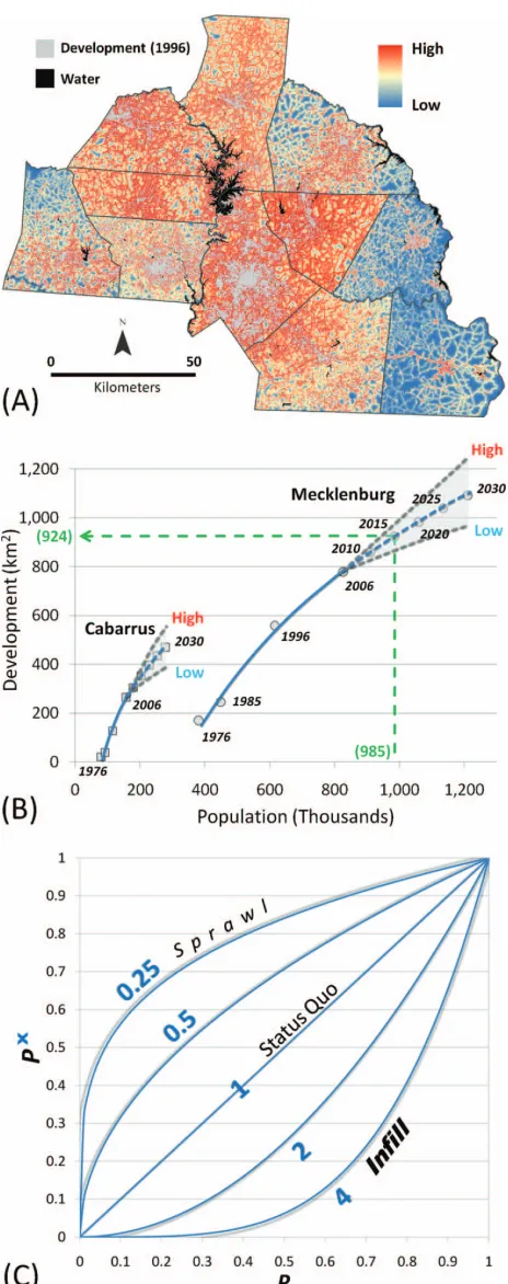
Figure 2. The Charlotte Metropolitan region located within (A) the “Char-lanta” megalopolis in the Southeastern United States. (B) The study system gained 8.3 percent developed land between 1996 and 2006 and was 24 percent developed by 2006 with substantial remaining tracts of forest and farmland. (C) Cabarrus County (FUTURES calibration site) exhibits a clear urban–rural gradient with growth rates and patterns representative of the study system. (Color figure available online.)
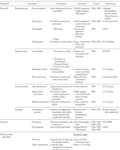
Figure 3. (A) Spatially explicit surface of the development poten-tial submodel (POTENTIAL) ranges from high (red) to low (blue) development likelihood. Gray denotes development as of 1996. (B) County-level forecasts of per capita land consumption (DEMAND). Status quo trendlines are shown in blue. Gray dashed lines denote alternative scenarios of land consumption. (C) Range of power func-tions (INCENTIVES) for transforming the development potential (P) surface. (Color figure available online.)
DEMAND: Per Capita Demand for Development by Level
DEMAND estimates the rate of per capita land con-sumption specific to each subregion or level (e.g., Figure 3B). Forecasts of land consumption are based on extrap-olations between historical changes in population and land conversion given expected or hypothetical scenar-ios of future population growth. Either prescribed or statistical approaches can be used to construct the per capita demand relationship for any level of population aggregation (e.g., county, census tract, census block), depending on the user’s preferred level of observation or data availability. Inputs for land area converted over a given time interval can be obtained through change analysis of existing maps (e.g., National Land Cover Dataset) or custom analysis of remote sensing data (see the section “Remote Sensing of Land Change” later in this article). Projections of land consumption at subregional extents reduce assumptions of stationarity and prescribe how much land to convert at a given time step.
PGA: Patch-Growing Algorithm
The PGA is a stochastic simulation that maps the allocation and spatial structure of land change using iterative site selection and a contextually aware region growing mechanism that changes cells from “undevel-oped” to terminal “devel“undevel-oped” states. PGA constructs conversion event objects by combining cell- and object-based representations of land change. Developed cells organize themselves over time into new patches of pre-scribed sizes and shapes, which can further aggregate into superpatches. Simulations of change at each time step feed development pressure back to the POTEN-TIAL submodel, influencing site suitability. Proxies for nonrationalities or human agency enter PGA as stochastic elements (Garc´ıa et al. 2011) that influence both site selection and patch configuration.
For a given time interval, patches are constructed in three steps. First, a seed for the initiation of a patch is al-located randomly across the POTENTIAL probability gradient. Using a Monte Carlo approach, this seed sur-vives if the probability value in POTENTIAL is larger than a random number (0–1). Allocation and selection processes are repeated until a seed survives and its resi-dent cell is selected to convert. Second, PGA examines the POTENTIAL suitability of contiguous cells and the spatial context of the cells in relation to the seed cell using a four-neighbor search rule. The inclusion of a cell (cell i) within a growing patch is determined
by a composite suitability score, denoted as si in Equation 1.
si =si∗d−α (1)
wheresiis the underlying development potential of the cell in question,dis its distance from the seed cell, andα is an adjustable scaling factor that controls patch com-pactness through a distance decay effect—that is,α in this equation is the parameter of patch compactness. As α increases, cells closer to the initial seed become rel-atively more attractive, promoting compact patch pro-duction. The composite score of each cell is then listed and ranked for each candidate neighbor cell. Third, PGA uses these ranked candidate cells to guide the neighborhood search for further patch growth; this pro-cess continues until a stopping criterion is met, such as patch size or total composite score (which can be informed by data on historical development), and the aggregate, contiguous cells are converted to a “changed” state. Conversion trajectory is assumed to be unidirec-tional: Once a cell is converted it remains in a static developed state. PGA continues to allocate patches un-til the per capita land DEMAND for growth is satisfied. The PGA approach provides a stochastic alternative to deterministic region-growing algorithms often used in site selection and conservation planning (Church et al. 2003).
Development pressure is a dynamic spatial variable derived from the patch-building process of PGA and associated with the POTENTIAL submodel. It is used to estimate the influence of surrounding land devel-opment on the likelihood that a cell changes states. The development pressure (noted as pi in Equation 2) on celliis given by:
pi = ni
k=1
Statek/di kγ (2)
whereStatekis a binary variable that indicates whether the kth neighboring cell is developed (1) or undevel-oped (0),dikis the distance between thekth neighboring cell and the current celli,γ is a coefficient that controls the influence of distance between neighboring cells and celli, andniis the number of neighboring cells within a specific range with respect to celli.Assuming the in-fluence of a neighboring developed cell on the current cell is distance-decayed, the development pressure on an undeveloped cell is a function of neighboring de-veloped cells and the distance between these cells and the cell in question. At each time step, PGA updates
the POTENTIAL probability gradient as land change events occur, and the new development pressure in turn affects future land change in a path-dependent man-ner with positive feedbacks (Brown, Page, et al. 2005). Because stochastic path-dependent systems are sensi-tive to initial conditions (Brown, Page, et al. 2005), we programmed PGA to produce multiple outcomes from a series of independent runs with model performance metrics reported as mean values.
User-set parameters within the PGA submodel al-low FUTURES to be calibrated for accuracy and used to explore alternative futures of urbanization and land-scape fragmentation (Table 1). For example, the patch compactness parameter (i.e.,αin Equation 1) allows a user to control the spatial complexity of patch shapes produced during the region growing process by influ-encing the amount of exploration in the neighborhood search mechanism. Scenarios involving policies that encourage infill versus sprawl can be explored using the incentive parameter, which uses a power function to transform the evenness of the probability gradient in POTENTIAL (Figure 3C). This transformation al-lows users to increase or decrease the likelihood of land change by altering site suitability in planning scenarios. The degree to which incentive transforms urban form and patterns of landscape fragmentation is assessed in our application of FUTURES later.
Model Application
We used FUTURES to project scenarios of land change in the metropolitan region of Charlotte, North Carolina, between 2006 and 2030. We first describe the methodologies that enable FUTURES to produce projections of forest and farmland conversion given a continuation of historical trends, including our data selection, analytical approaches, and calibration proce-dures. We then evaluated FUTURES’s performance in simulating change between 1996 and 2006 using cell-based metrics of error due to quantity and error due to allocation (Chen and Pontius 2010) and patch-based metrics of spatial structure along an urban–rural gra-dient. We conclude with three simulation experiments designed to demonstrate the capability of FUTURES to analyze alternative futures of urban form and landscape fragmentation.
Study System
Located in the middle of the “Char-lanta” megalopo-lis, the third largest megaregion in the United States
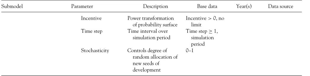
Table 1. FUTURES submodel parameters
Submodel Parameter Description Base data Year(s) Data source
Potential Environmental Forest-farmland Lands designated as forest or farmland
LiDAR vegetation height; Landsat TM imagery
1996, 2006 Charlotte-Mecklenburg County Storm Water Services; USGS Open space Proximity to protected
open space
Lands managed for conservation and open space
1996, 2006 Conservision-NC
Topography 1. Elevation 1-arc second
National Elevation Dataset
2006 USGS
2. Slope
Hydrography Proximity to water bodies Rivers, recreational lakes, and reservoirs
1996, 2006 NC OneMapa
Infrastructural Accessibility 1. Proximity to roads Primary and secondary road networks
1996 NCDOT
2. Proximity to interchanges 3. Density of roads 4. Travel cost (time) Municipal centers Proximity to
municipalities
Locations of cities, towns, and other municipalities
1996 U.S. Census
Water and sewer Proximity to water and sewer service lines
Water Services Assessment database
1996 Conservision-NC
Socioeconomic Age and income Age/income structure and distribution
Census statistics 1996 U.S. Census
Employment attraction
Proximity to urban centers weighted by number of jobs provided
Traffic analysis zone (TAZ) and place-of-work statistics
1996 U.S. Census
Multilevel structure Proxy for varying policy effects
Census statistical geographies
1996 U.S. Census
Dynamic Development
pressure
Number of neighboring developed cells within search distance and weighted by distance
Historical and forecast development patterns
1996–2030 Remote sensing and simulationsb
Demand Population Historical population and
projections
State demographic data
1976, 1985, 1996–2030
NCOSBM
Development Area of developed land Landsat MSS & TM imagery
1976, 1985, 1996, 2006
USGS
Patch-growing algorithm
Parameter range
Patch size Controls area of each new development patch
Area≥0.09 ha, total region area Patch compactness Controls shape
complexity of each new development patch
Shape≥1, no limit
(Continued on next page)
Table 1. FUTURES submodel parameters(Continued)
Submodel Parameter Description Base data Year(s) Data source
Incentive Power transformation
of probability surface
Incentive>0, no limit
Time step Time interval over
simulation period
Time step≥1, simulation period Stochasticity Controls degree of
random allocation of new seeds of development
0–1
Note:LiDAR=light detection and ranging; USGS=United States Geological Survey (www.usgs.gov); Conservision-NC=One NC Naturally’s Con-servation Planning Tool (www.conservision-nc.net); NCDOT=North Carolina Department of Transportation (www.ncdot.org); U.S. Census=United States Census Bureau (www.census.gov); NCOSBM = State Demographics Branch of the North Carolina Office of State Budget and Management (http://www.osbm.state.nc.us/).
aNorth Carolina ONEmap is distributed by the North Carolina Center for Geographic Information & Analysis (www.nconemap.com). bLandsat satellite image analysis and FUTURES simulations.
(Florida, Gulden, and Mellander 2008; see Figure 2A), Charlotte is a rapidly growing metropolitan area and the major economic hub for the eleven-county, 13,400 km2 study region (Figure 2B). Charlotte is situated in the center of the Southern Piedmont province, a biologi-cally diverse and productive ecoregion that still supports large areas of forest and farmland. Home to more than 2 million people (North Carolina Office of State Bud-get and Management [NCOSBM] 2010), the region’s rolling landscape is connected via a high-speed inter-state system and has some of the highest densities of sec-ondary and tertiary road networks in the United States. The region holds few environmental obstacles for devel-opment, and with the exception of impounded river sys-tems to the east and west, there are no geographic bar-riers. In this strong property rights state (Wang, Thill, and Meentemeyer 2012), planning is primarily imple-mented through zoning; alternative controls such as adequate public facility ordinances have not been sup-ported by the state judiciary. Despite recent economic recession conditions, Charlotte–Mecklenburg and its ten surrounding North Carolina counties are projected to gain nearly 700,000 people by 2030, a 30 percent increase in population (NCOSBM 2010).
Remote Sensing of Land Change
We developed an empirical understanding of trends in land change by tracking urban and rural develop-ment over four decadal time steps (1976, 1985, 1996, and 2006) from three data sources: moderate-resolution Landsat MSS and TM satellite imagery, aerial or-thophotography, and high-resolution light detection
and ranging data (LiDAR). We used three sequential procedures to classify remote sensing data into three terrestrial land cover classes (development, forest, and farmland) at each time step: (1) subpixel modeling of Landsat data into vegetation–impervious surface–soil (VIS) fraction components (Lee and Lathrop 2005; Gluch and Ridd 2010), (2) classification of developed and undeveloped land covers from the VIS fractions with manual correction using orthophotography, and (3) further discrimination of spectrally similar forest and farmland vegetation within the undeveloped class using vegetation structure data derived from LiDAR. We mapped patterns of land cover change ourselves because the study system contains numerous areas of low-density land cover types prone to misclassification by commonly used land cover data such as the National Land Cover Dataset (Irwin and Bockstael 2007).
In the first step, we used VIS modeling and uncon-strained linear spectral unmixing analysis to produce fractional components representing the relative pro-portion of vegetation, impervious surfaces, and soil for each Landsat image pixel (Lee and Lathrop 2005). Im-age preprocessing included both radiometric calibration of image data to at-sensor reflectance and across-band brightness normalization (C. S. Wu 2004). We used aerial orthophotography to select training sites repre-senting pure end members for green vegetation, imper-vious surfaces, and exposed soil. The spectral unmixing process generated representative fractional images of the region that were rescaled to sum to one.
Second, we used logistic regression to classify the continuous VIS fractions into developed or undevel-oped categories based on interpretation of 550 points
in concurrent 2006 orthophotography. The two-class system reduces the likelihood of error as compared to three or more classes (Pontius and Malizia 2004). We classified agricultural lands and industrial forests as un-developed, whereas highly managed “green” areas, such as golf courses and irrigated lawns, were assigned to the developed class. We then used heads-up digitizing to correct obvious misclassifications.
Third, we further distinguished forest and farmland types of undeveloped land cover using LiDAR data col-lected in 2004. Our model of vegetation height derived from the first and last LiDAR returns clearly discrim-inated forests from farmlands (Singh et al. forthcom-ing). Within a geographic information system (GIS), we used the height model in overlay analysis to update the 1996 land cover maps under the reasonable assump-tion that forests in 2006 were also forested in 1996. We assessed map accuracy using concurrent high-resolution aerial photography. For each time step, we evaluated a total of 150 randomly located points for the presence of development per satellite image. Overall accuracy for classifications ranged from 78 percent (1976) to 86 percent (2006).
Our analysis of historical imagery revealed rapid and extensive conversions of agricultural and natural land-scapes between 1976 and 2006. During the thirty-year period, more than 280,000 ha of forest and farmlands converted to developed land, increasing the total built environment to 24 percent of the nonwater area. Lands converted at a rate of 35 ha per day between 1985 and 1996 and 32.5 ha per day between 1996 and 2006.
Development Potential Submodel (POTENTIAL)
To build the multilevel statistical model, we devel-oped a response variable based on conversions of un-developed to un-developed lands identified from remote sensing between 1996 and 2006. Analysis revealed that this period (1996–2006) experienced robust yet slow-ing growth preceded by a decade (1985–1996) of rapid expansion. We assumed that factors driving develop-ment suitability during the more recent decade would also drive suitability for the period of projection. We generated a binary, developed–undeveloped response variable using a stratified-random sample of 1,450 grid cells distributed across the eleven-county study extent (n=848 transitioning cells;n=602 forest and farm-land cells). We excluded from analysis all water bodies and areas protected from development (e.g., no-build buffers, conservation areas). Prior to fitting the model, we selected a set of significant (p<0.05) and
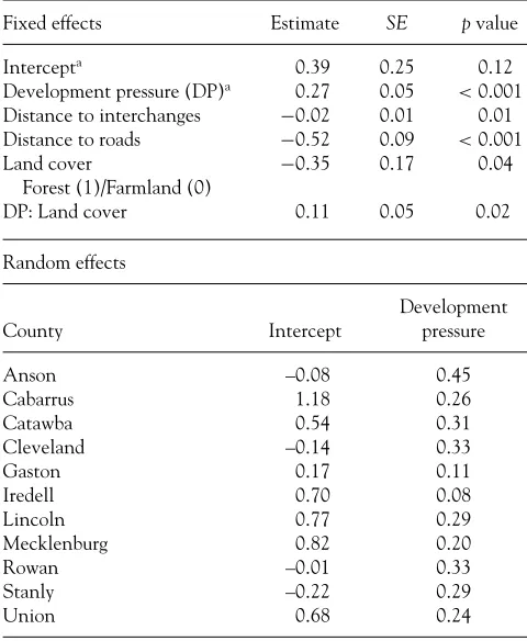
uncorre-Table 2. Results of generalized linear mixed model: Fixed effects including interaction between development pressure and land cover followed by random effects for intercept and
development pressure which vary by county
Fixed effects Estimate SE pvalue
Intercepta 0.39 0.25 0.12
Development pressure (DP)a 0.27 0.05 <0.001
Distance to interchanges −0.02 0.01 0.01
Distance to roads −0.52 0.09 <0.001
Land cover −0.35 0.17 0.04
Forest (1)/Farmland (0)
DP: Land cover 0.11 0.05 0.02
Random effects
Development
County Intercept pressure
Anson –0.08 0.45
Cabarrus 1.18 0.26
Catawba 0.54 0.31
Cleveland –0.14 0.33
Gaston 0.17 0.11
Iredell 0.70 0.08
Lincoln 0.77 0.29
Mecklenburg 0.82 0.20
Rowan –0.01 0.33
Stanly –0.22 0.29
Union 0.68 0.24
Note: SE=standard error.
aVaries by county, see random effects.
lated predictors of change from our initial list of hypoth-esized site suitability variables (Table 1) using forward and backward stepwise regression techniques. We also tested for a hypothesized interaction between develop-ment pressure and land cover (forest vs. farmland). We included “county” as the group-level indicator in the multilevel model to account for spatially nonstation-ary processes inherent across jurisdictional boundaries. The varying intercept-varying slope model explained overall differences in development potential as well as variation in relationships between potential and the predictors among counties. Here, we allowed only the slope of the development pressure variable to differ by county (Table 2).
We used Laplace approximation, suitable for multi-level modeling with binary response variables (Bolker et al. 2009), to estimate model parameters with the lme4 package (Bates and Maechler 2009) in R Version 2.10.0 (R Development Core Team 2009). The probability,p,
that an undeveloped cell,i, becomes developed is
pi = esi
1+esi (3)
where si is the composite development potential for cell iin Equation 1, which is a function of the origi-nal development potentialsi and distanced.Further, the original development potential siis a function of environmental, infrastructural, and socioeconomic pre-dictor variables of site suitability (Table 1). Specifically, in this study,siis described by:
si =aj[i]+ n
h=1
βj[i]h ∗xi h +βj[i]∗pi (4)
where, for theith undeveloped cell and varying acrossj groups (i.e., the level),aj[i]is the intercept,βj[i]is the re-gression coefficient,his a predictor variable represent-ing conditions in 1996, n is the number of predictor variables, xih is the value of h at i, and pi is the dy-namic development pressure variable (see Equation 2). We determined the value of the development pressure variable by running the statistical analysis for values of γ ranging from 1 to 100 and choosing the value (γ = 1.8) that resulted in peak model performance based on likelihood profile estimates (Hilborn and Mangel 1997; Meentemeyer et al. 2008).
Overall model results indicated that the probability of development was greatest in farmlands surrounded by high development pressure and close to roads and highway interchanges (Table 2). As development pres-sure increased, there was a shift toward greater prob-ability of development in forested areas close to road networks. Because we implemented a multilevel model to establish these relationships, the effect of develop-ment pressure varies spatially with unique, county-level parameter estimates for β (Table 2). We applied the most parsimonious multilevel model (Table 2) to the mapped predictor variables in the GIS to produce a spatially explicit surface of development potential for initiating simulations (POTENTIAL; Figure 3A).
Land Demand Submodel (DEMAND)
We projected future rates of per capita land con-sumption (DEMAND) based on relationships between trends in population growth and demand for develop-ment that occurred between 1976 and 2006 (Figure 3B). For each of our historical time steps (1976, 1985, 1996, and 2006), we obtained county-level population totals
from the State Demographics Branch of the NCOSBM. We acquired annual projections of population growth by county through the year 2030 from the same source. For each of the eleven counties, we used ordinary least squares regression—allowing for linear or logarithmic relationships—to estimate a “best fit” model of pop-ulation versus area of development (1976–2006) as mapped from our remote sensing of land change. We then used each regression equation to extrapolate per capita land consumption through 2030 based on fu-ture population projections (Figure 3B). Forecasts of land consumption provided by the submodel DEMAND drive the rate of development in the PGA submodel for the simulation of future land development.
Calibration of the PGA
We used empirical distributions of patch size and shape metrics (compactness, as defined later) of new development patterns identified in our analysis of 1996 and 2006 imagery as references to calibrate our model. We assumed that the factors driving spatial configura-tion of development events during this period would continue throughout the period of projection. Starting with 1996, we conducted simulations at one-year time steps, assuming that an equal number of cells converted into development each year.
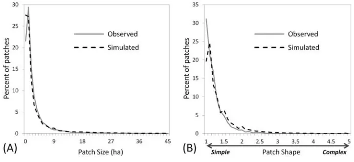
To calibrate PGA’s annual simulations of develop-ment events, we first derived simulated distributions of patch size and shape that, when accreted over ten years, closely matched observed patch metrics. We derived the patch size distribution for our simulation model fs i m by converting the empirical distribution of patch size fobs, using:
fs i m(ps i ze)=θ ∗ fobs(ps i ze) (5)
whereθ is a discounted factor that varies between zero and one, andpsizeis the variable of patch size (Table 1). We compared a range of ten-year simulation outcomes generated by various discount factors and tunedθto 0.6 to obtain reasonable agreement between simulated and observed patch size (Figure 4A).
The shape metric (noted asSHAPE) used in calibra-tion was defined as:
SHAPE= Pk/min Pk (6)
wherePkis the perimeter of patchk, andmin Pkis the perimeter of a circle given the same patch area (see McGarigal et al. 2002).
Figure 4. Calibration of FUTURES patch-growing algorithm (PGA). Fre-quency distributions for calibrated landscape show strong agreement be-tween simulated and observed patch (A) size and (B) shape metrics.
We analyzed the mean output of fifty stochastic re-alizations and iteratively adjusted the patch compact-ness parameterα(Equation 1) until the distribution of simulated and observed patch shape matched closely (Figure 4B). Comparison of histograms of the shape in-dex between simulated and observed patterns was used to support shape calibration (Figure 4B). The range of the patch compactness parameter α was calibrated to [0.32, 0.48], where a uniform distribution was used to draw distributed values ofα to generate alternative shape parameters for patches to be simulated. For this application, we reduced computational complexity by parameterizing PGA’s patch-building capabilities using a representative region of the metropolitan area (Cabar-rus County; Figure 2C), though FUTURES’ multilevel structure allows patch characteristics to be calibrated separately for all levels in the model. The urban–rural continuum across Cabarrus County encompasses the range of patch characteristics across the study region (Figure 4).
FUTURES Model Performance
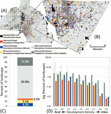
We applied the calibrated version of FUTURES to simulate land change between 1996 and 2006 in the eleven-county region and assessed its ability to sim-ulate patterns of urban, suburban, and rural develop-ment. Because FUTURES aggregates cell-level change to produce patches of land change events, we evalu-ated the geographical variation of simulations—based on the mean of fifty stochastic model runs—using both cell- and patch-level diagnostics along an urban–rural gradient instituted by imposing a 6 km×6 km lattice over the study area (Figure 5A; Figure 5B for detail) and ranking each lattice block by percentage of developed
lands as of 1996, hereafter referred to as thedevelopment density gradient.
We conducted model diagnostics recommended by Chen and Pontius (2010) with one modification: We partitioned null successes into eligible and ineligible categories to reflect heuristics that prevent FUTURES from simulating growth in developed areas (Figure 5). FUTURES simulated 9.2 percent change for the rurally biased study extent (Figure 5C), whereas ob-served change was 8.3 percent. On average, hits (2.1 percent) and combined null successes (84.6 percent) constituted 86.7 percent of the landscape. Figure of merit, the measure of statistical agreement between ob-served and simulated change (Pontius et al. 2008), was 13.6 percent. Assessing simulated landscape composi-tion relative to development density aggregated on the 6 km × 6 km lattice revealed a relative evenness in correctness and error of simulated change except in the most rural areas (Figure 5D).
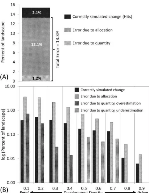
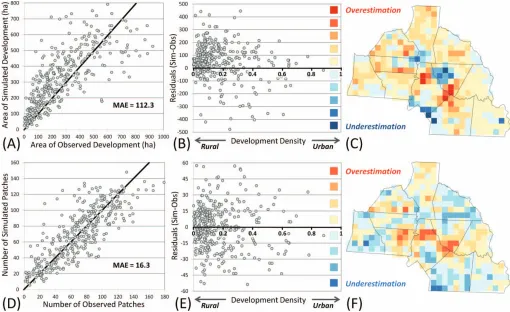
Evaluation of cell-based change revealed error due to quantity (1.2 percent) and error due to allocation (12.1 percent) totaling 13.3 percent of the landscape on average (Figure 6A). Distribution of these errors along the development density gradient indicates that FUTURES slightly overestimates development in rural areas and underestimates in more urban settings (Fig-ure 6B). Our patch-level assessment of spatial struct(Fig-ure first compared the area of observed patches to the area of simulated patches of new development, averaged by block. With respect to both the one-to-one line of per-fect agreement and the development density gradient, results indicate a bias in model performance for overesti-mating patch area in more rural settings (Figures 7A, 7B, and 7C). The number of patches constructed showed a stronger correspondence between observed and simu-lated with respect to the one-to-one line and along the
Figure 5. Cell-level model perfor-mance based on simulation successes and errors across study system. (A) Spatial distribution of successes and errors comparing 1996–2006 observed and simulated change. The 6×6 km lattice (white grid) used to analyze suc-cesses and errors by block and along de-velopment density gradient. (B) Suc-cesses and errors in Cabarrus County. (C) Proportions of successes and errors for entire landscape. (D) Distribution of block-summarized successes and er-rors along development density gradi-ent (bin interval of 0.1). Map legend also applies to (C) and (D) with the exception of excluded water and pro-tected open space. (Color figure avail-able online.)
development density gradient. Mapped residuals cor-roborate these findings (Figures 7D, 7E, and 7F).
Simulation Experiments
Forest and agricultural landscapes along urban– exurban gradients are often highly fragmented, with compromised productivity and ecosystem function compared to their bucolic counterparts; nonetheless, these remnant landscapes are vital repositories of cultural practice, refuges of natural heritage and biodiversity, and essential providers of clean air, wa-ter, and open space (McDonnell and Pickett 1990; Bol-und and Hunhammar 1999). Despite the recognition of these ecosystem services, policies designed to man-age unsustainable growth have been largely ineffective (Anthony 2004; Howell-Moroney 2007). Researchers of coupled human–natural systems are increasingly rec-ognizing the value of using land change models to
ex-plore potential impacts of growth on future landscapes (B. L. Turner, Lambin, and Reenberg 2007). Inquiry-and strategy-driven projections of long-term societal and environmental change allow stakeholders to test planning and policy interventions long before imple-mentation (Alcamo 2008) and across large spatial scales that cross municipal boundaries and stakeholder prior-ities. Yet little is known about the efficacy of growth management approaches to minimizing fragmentation of natural areas due to a paucity of applied case his-tories and the challenge of simulating fragmented spa-tial structures as exemplified by parcel-based analyses by Irwin, Bell, and Geoghegan (2003) and Irwin and Bockstael (2004).
We used FUTURES to evaluate the emergence of landscape spatial structure in response to two hypoth-esized growth management approaches in the rapidly urbanizing Charlotte metropolitan region and com-pared those outcomes to projected patterns based on recent development trajectories. Our simulation
Figure 6. Cell-level model performance based on accuracy of sim-ulated change (1996–2006) across study system. (A) Proportions of errors and correctly simulated change for entire landscape. (B) Distribution of errors and correctly simulated change along devel-opment density gradient (bin interval of 0.1). Overestimation in-dicates false alarms>misses; underestimation indicates false alarms <misses. Missing bars indicate no error in category.
experiments were conducted over a twenty-five-year period (2006–2030) using the calibrated version of FU-TURES where (1) the region continued the status quo trend of growth observed between 1996 and 2006; (2) per capita land consumption varied above and below rates observed prior to 2006 using the DEMAND sub-model (Figure 3B); and (3) we transformed develop-ment suitability using the INCENTIVE parameter to examine the change in the distribution and spatial structure of new patches across the landscape (Figure 3C). At the end of each experiment, we quantified changes to the spatial structure of forest and farmland resources through 2030 using the landscape metrics soft-ware, FRAGSTATS (McGarigal et al. 2002), which aggregated pixels into patches based on a four-neighbor rule and measured the area, number, and shape com-plexity of new patches (Equation 6). We assumed sta-tionarity in process during the projection period—that is, the simulation of new patches of development (patch
size and patch shape) would closely emulate the ob-served size and shape characteristics of patches formed during the 1996 to 2006 historical time period (Figure 4)— to establish status quo benchmarks for comparison to alternative development outcomes.
Benchmark: Historical Trajectory of Landscape Change
To establish a benchmark, we first projected urban growth in the eleven-county region through 2030 based on the continuation of land consumption trends observed between 1996 and 2006. This period is noteworthy for Charlotte because the land grab that occurred in the previous decade (1985–1996) slowed from 35 ha per day to 32.5 ha per day, given similar economic conditions and a maturing of the land devel-opment market. During this period, immigration to the region remained strong and increased linearly (Figure 3B). Expansion of Charlotte’s transportation beltway I-485 during this period lowered mean commute times to twenty-eight minutes but increased access to undeveloped lands (Charlotte Chamber of Commerce 2011).
FUTURES projected that continued growth trends will convert an additional 212,650 ha of forest and farm-land by 2030, increasing developed farm-land use from 24 percent to 41 percent of the nonwater landscape (see Figure 8A for detailed map). Projections of the rate of development show a continuation of the slowing trend, from an average of 27 ha per day between 2007 and 2016 to 21 ha per day by 2030. Many undeveloped ar-eas experience substantially more fragmentation: Forest remnants become smaller (9.7 ha vs. 17.8 ha), more nu-merous (52,467 vs. 38,602), and slightly more complex in shape (1.24 vs. 1.22) in 2030 than in 2006, on av-erage (see SQ values in Table 3). Farmland responds somewhat differently to projected growth: Patches be-come smaller on average (2.9 ha vs. 4.5 ha) but sim-ilar in number (88,413 vs. 90,000) and shape (1.22 vs. 1.24).
Landscape Response to Per Capita Land Consumption
We simulated growth patterns over the benchmark period (1996–2030) using a range of per capita land consumption rates parameterized within the DEMAND submodel. High projections of land consumption as-sume that new populations demand more land per per-son than currently experienced; low projections assume
Figure 7. Patch-level model performance comparing 1996–2006 observed and simulated patch area and number of patches, summarized by blocks across study system. (A) Total patch area (ha) of observed and simulated development plotted along one-to-one line and with mean absolute error (MAE) reported. (B) Residuals of total area (ha) of development plotted along development density gradient and (C) spatial distribution of residuals indicate overestimates in North and East Charlotte and rural areas. (D) Number of observed and simulated patches of development plotted along one-to-one line and with MAE reported. (E) Residuals of number of patches of development plotted along development density gradient and (F) spatial distribution of residuals indicate over- and underestimation vary across region with overestimates in transitioning areas of North and East Charlotte. Blocks with>50 percent of area beyond study system boundary were excluded. (Color figure available online.)
each individual uses less land (Figure 3B). Treatments ranged from 40 percent below levels observed between 1996 and 2006 to 40 percent above (Table 3). We made changes to per capita land consumption at the county level and held all other factors constant, including de-velopment suitability and PGA parameterizations. For each treatment, we ran FUTURES fifty times to pro-vide more reliable estimates of mean behavior. We con-ducted patch analyses for each simulation with average values reported.
Reducing per capita consumption by 40 percent, from an average of 0.80 ha per person to 0.48 ha per per-son, retained more than 38,500 ha of forest and 27,100 ha of farmland region-wide by 2030, conserving 19 per-cent of the total green space as compared to losses antic-ipated by the historical trend (Table 3 and Figure 8B). Reductions in consumption also minimized
fragmenta-tion of forests as indicated by fewer patches and larger patch areas. Farmlands were also conserved with re-ductions in per capita consumption, but whereas patch area increased, the number of patches also increased (Table 3). Elevated levels of per capita consumption ex-pectedly increased losses of forest and farmlands above the historical trends (Table 3 and Figure 8B).
Impacts of INCENTIVE on Development Distribution
We explored landscape responses to hypothesized growth management practices that reward or discourage the placement of new development by changing the relative attractiveness of undeveloped lands. Cluster-ing new development near existCluster-ing infrastructure has the potential to reduce service costs (Carruthers and
Table 3 . Impacts o f varying per capita land consumption (PCLC), 1996–2030 Development Forest F armland PCLC multiplier A rea a No. of patches
Mean patch area Mean patch shape
A rea a No. of patches
Mean patch area Mean patch shape
A rea a No. of patches
Mean patch area
1.4 614 , 236 (12%) 2 7 , 692 (–10%) 1 4 . 4 (34%) 1 . 464 468 , 178 (–8%) 5 6 , 030 (7%) 8 . 4 (–14%) 1 . 233 231 , 479 (–10%) 8 6 , 032 (–3%) 2 . 69 (–8%) 1.2 580 , 798 (6%) 29 , 331 (–4%) 1 2 . 5 (16%) 1 . 464 488 , 483 (–4%) 5 4 , 153 (3%) 9 . 0 (–7%) 1 . 240 244 , 230 (–5%) 8 7 , 389 (–1%) 2 . 79 (–4%) SQ 547 , 402 30 , 819 10 . 81 . 462 508 , 245 52,467 9 . 71 . 243 257 , 465 88 , 413 2 . 91 0.8 514 , 056 (–6%) 3 1 , 813 (3%) 9 . 4 (–13%) 1 . 458 527 , 604 (4%) 50 , 765 (–3%) 1 0 . 4( 7 % ) 1 . 245 271 , 010 (5%) 89 , 085 (1%) 3 . 04 (4%) 0.6 480 , 611 (–12%) 3 2 , 501 (5%) 8 . 2 (–24%) 1 . 448 546 , 915 (8%) 49 , 181 (–6%) 1 1 . 1 (15%) 1 . 245 284 , 659 (11%) 8 9 , 938 (2%) 3 . 17 (9%) Note: Area in h ectares; p ercent change from status quo (SQ = 1) in parentheses. aTotal area for land covers ranges 1,708 ha (0.13 p ercent) from median due to data processing. 15
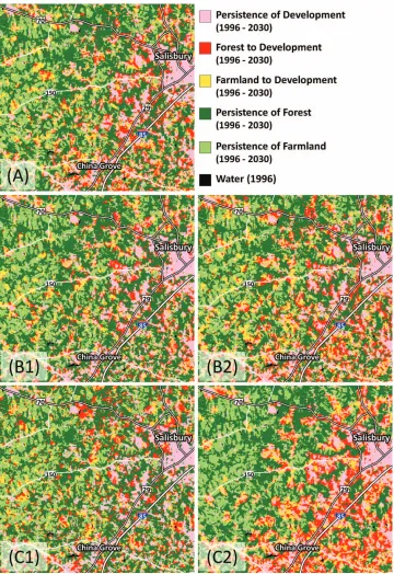
Figure 8. Detail views (20 km × 20 km region of Rowan County) of land change projections (1996–2030) based on three simulation exper-iments. (A) Experiment 1: Con-tinuation of observed (1996–2006) land consumption trends (status quo). Experiment 2 (impacts of per capita land consumption [PCLC]): Develop-ment density treatDevelop-ments ranged from (B1) 40 percent reduction in PCLC below observed rates (1996–2006) to (B2) 40 percent increase in PCLC above observed rates. Experiment 3 (impacts of locational INCENTIVE): Development potential gradient var-ied by adjusting INCENTIVE in treat-ments ranging from (C1) 0.25 (low in-fill incentive, greater sprawl) to (C2) 4.0 (high infill incentive, greater in-fill). (Color figure available online.)
Ulfarsson 2003), ease congestion and pollution associ-ated with vehicle emissions (U.S. Environmental Pro-tection Agency [EPA] 2001), and conserve forests and farmlands by reducing disjunct or leapfrog develop-ment. In practice, development suitability could be al-tered through disincentives such as the establishment of “growth boundaries” beyond which municipalities restrict or deny provisioning of sewer and water
sys-tems to new settlement or economic incentives such as priority funding areas (PFAs) that promote infill over greenfield development (Cohen 2002). We used the IN-CENTIVES parameter (Figure 3C) as a simple regional proxy for varying POTENTIAL and evaluated land-scape response to projected growth through the year 2030. INCENTIVE modifies the evenness of the em-pirically derived POTENTIAL development suitability
surface, thereby changing the survival likelihood of patch-starting seeds, an effect that in turn modifies the distribution of patches. We applied five treatments ranging from 0.25 (sprawl), which flattened develop-ment suitability, to 4.0 (infill), which attenuated devel-opment suitability. We held all other factors constant, including population projections, per capita land con-sumption, and the PGA parameterizations. For each treatment, we ran FUTURES fifty times to characterize stochasticity of human agency in land change dynam-ics. We conducted patch analyses for each simulation with average values reported.
Simulations with lower INCENTIVE treatments re-sulted in diffuse growth (Figure 8C), with increased fragmentation indicated by more patches of develop-ment, forest, and farmland and reduced patch size for development and forest (Table 4). In contrast, simu-lations with higher INCENTIVE treatments increased the relative suitability of undeveloped areas near ex-tant high suitability (e.g., areas with high develop-ment pressure and close to roads and highway in-terchanges), resulting in more compact urban growth (Figure 8C), which reduced fragmentation of forest and farmland when compared with projections of histori-cal trends (Table 4 and Figure 8A). Although higher INCENTIVE treatments resulted in small changes (±1 percent) in both forest and farmland relative to sta-tus quo historical growth, lower INCENTIVE values unexpectedly consumed forests while preserving farm-lands, with forests losing 18,000 ha (–3.6 percent) and farmlands retaining 4,400 ha (6.2 percent) com-pared to the status quo historical trend (Table 4 and Figure 9).
Discussion
Societies structure landscapes in patterns that result from complex combinations of decision processes (B¨urgi and Turner 2002), driving forces (B¨urgi, Hersperger, and Schneeberger 2004), and chance (Pontius and Spencer 2005), the results of which are manifested as a continuum of conversion events that consume and frag-ment undeveloped lands. Over time these processes are reciprocally influenced by the structures they create and agglomerate to produce regional settlement patterns. Here we present a methodology that diminishes the fun-damental land change modeling dichotomy, whether process drives pattern or pattern drives process, by first reconciling the arbitrary process entity (cell, or grain)
Figure 9. Differential response of forest and farmland to varying the locational INCENTIVE parameter.
with the structural object (land conversion events) and then building feedbacks between simulated structures and process-based transition probabilities. When ap-plied to a series of hypothesized growth management treatments, FUTURES projected regional scenarios of land change that produced spatial structures of urban-ization and fragmentation at landscape scales.
Multilevel structure is another characteristic that makes FUTURES appropriate for modeling land change dynamics at regional extents (Irwin, Jayaprakash, and Munroe 2009). Analysis of change at the subregional level (county) allowed us to account for socioeconomic and policy factors that vary across a region but that are not typically available as geospatial data (Fotheringham and Brunsdon 1999). The implementation of multilevel modeling also allowed relationships to diverge and vary spatially, rather than assuming stationarity across the entire metropolitan region (Gelman and Hill 2007).
Table 4 . Impacts o f varying locational incentives (infill v s. sprawl), 1996–2030 Development a Forest F armland Exponent No. of patches Mean patch area
Mean patch shape
A rea b No. of patches
Mean patch area Mean patch shape
A rea b No. of patches
Mean patch area
Sprawl 0 . 25 47 , 445 (54%) 7 . 0 (–35%) 1 . 264 489 , 827 (–3 . 6%) 5 8 , 857 (12%) 8 . 3 (–14%) 1 . 265 273 , 377 (6 . 2%) 9 2 , 991 (5%) 2 . 94 (1%) 0 . 54 1 , 560 (35%) 8 . 0 (–26%) 1 . 328 498 , 305 (–1 . 9%) 5 6 , 032 (7%) 8 . 9( – 8 % ) 1 . 260 265 , 877 (3 . 3%) 9 1 , 296 (3%) 2 . 91 (0%) SQ 30 , 766 10 . 81 . 463 508,173 52 , 511 9 . 71 . 243 257,497 88 , 381 2 . 91 21 7 , 721 (–42%) 1 8 . 8 (74%) 1 . 611 512 , 255 (0 . 8%) 4 7 , 433 (–10%) 1 0 . 8 (12%) 1 . 215 254 , 704 (–1 . 1%) 8 1 , 808 (–7%) 3 . 11 (7%) Infill 4 10 , 163 (–67%) 3 2 . 7 (203%) 1 . 688 509 , 641 (0 . 3%) 4 4 , 154 (–16%) 1 1 . 5 (19%) 1 . 181 257 , 846 (0 . 1%) 7 5 , 508 (–15%) 3 . 41 (17%) Note: Area in h ectares; p ercent change from status quo (SQ = 1) in parentheses. aArea o f d eveloped land consistent across all treatments at 544,280 ha. bTotal area for other land covers (forest, farmland) ranges 4,283 (0.33 p ercent) from median due to data processing. 18
Model Performance
To explore the effects of growth along urban–rural gradients, FUTURES was designed to simulate leapfrog and exurban development objects in areas with low development potential while still converting undevel-oped remnants in areas of high development suitability. These contrasting conversion events represent a mod-eling challenge in how best to allocate the limited num-ber of prescribed transitions to simulate both urban and exurban growth with acceptable accuracy while main-taining generic heuristics that avoid overfitting a model. In analyzing error, relative evenness in correctness and error along the development density gradient indicated that FUTURES simulated new development in low-and high-suitability areas; in contrast, clumping (e.g., correctness biased toward high-potential areas) would have indicated that the spatial allocation of conversion events was flawed even if overall accuracy was higher as a result.
Validation diagnostics for the entire landscape in-dicated that FUTURES produced an overall accuracy of 86.7 percent, a high value due in part to the major-ity of the landscape being persistent, undeveloped land cover (Figure 5). The figure of merit, a measure of sim-ulation accuracy, was 13.6 percent, a value consistent with other case studies where observed change is a rare event (e.g., less than 10 percent; Pontius et al. 2008). Analysis of error found 12.1 percent attributable to er-rors of allocation and 1.2 percent attributable to quanti-ties prescribed by the DEMAND submodel (Figure 6A). Classification error for the interval (20 percent in 1996, 14 percent in 2006) could also account for a propor-tion of cell error (Pontius and Lippitt 2006). Rela-tive evenness of error and correctness across the de-velopment density gradient (Figures 5D, 6B) support FUTURES’s applicability to simulating change over a range of regional contexts. Patch-level diagnostics ag-gregated from our regional lattice (6 km×6 km blocks) showed some rural bias between simulated and observed in terms of area of new patches of development (Figure 7A) and stronger correspondence in terms of the num-ber of new patches of development (Figure 7D). When residuals of patch area (Figure 7B) and number of new patches (Figure 7E) are plotted along the development density gradient, we see that the study system is skewed toward rural land covers, but error exhibits relative ho-moscedasticity. Mapped residuals shows overestimate in rapidly transitioning areas of North and East Charlotte (Figures 7C, 7F).
Our application of FUTURES covered a large geo-graphical extent (174 km × 140 km; Figure 2), with land change dynamics represented as cell- and patch-level mechanisms operating on a relatively fine spatial resolution (30 m×30 m). This spatial grain and extent made our application too computationally demanding for desktop computing environments to meet the re-quired compute time and memory capacity (Tang and Wang 2009). We necessarily used high-performance computing to conduct multiple stochastic simulation runs distributed across multiple advanced computing processors with large memory configuration in a paral-lel manner (Wilkinson and Allen 2004). Smaller study extents for calibration and simplifying the equation for calculating development pressure at each time step are two options for overcoming computational barriers if a high-performance computing infrastructure is not accessible.
Change in the Charlotte Region
Since the mid-1980s, the Charlotte region has ur-banized in disjoint, low-density patterns where over one third of an acre was developed for each regional occupant by 2006. Our DEMAND analyses revealed the alarming result that land conversions outpaced the doubling population. FUTURES projected additional losses of 212,650 ha of forested and agricultural land by the year 2030 if the trends exhibited between 1996 and 2006 persist. These trends are notable given the ongoing changes to infiltration zones, bioretention, and losses of evapotranspiration that have already led to the region’s primary source of drinking water and power, the Catawba River Basin, being named America’s most en-dangered river in 2008 by American Rivers (Hamilton, Kober, and Hewes 2008).
Charlotte’s high and rising land consumption rates match those of megaregion sibling Atlanta but, in con-trast, Charlotte’s larger amount of remaining forests and farmlands suggest that it is still early enough in its growth trajectory to plan a more environmentally benign future. Our simulations of alternative futures of reduced landscape fragmentation and expansion of impervious surfaces illustrate that the region still has viable options. Despite growing interest in open space and “green” development, however, little change in pol-icy is expected in the near term. North Carolina is a strong property rights state, with counties and munici-palities limited to a few planning instruments, such as temporary building moratoria, adequate public facility
ordinances (APFO), and zoning (Ott and Read 2006), the latter being routinely adjusted to landowners’ wishes once development pressure is high enough.
Simulation Experiments
When fragmentation is understood as an emergent behavior generated by a complex system of multiple and disparate forcings, evolving feedbacks, and nonlinear trajectories of cause and effect, bottom-up approaches offer new tools into a seemingly intractable situa-tion that confounds top-down, prescriptive approaches (Innes and Booher 1999). Given that current land use policy in the Charlotte region is unlikely to reduce frag-mentation and its associated impacts, we explored the effects of two bottom-up treatments using simple global parameters that we view as proxies for market-based planning tools. Scenarios that lowered per capita land consumption, ostensibly through “upzoning” or density entitlements that permit builders to place more units per area, were revealed to conserve forest and farmland and reduce forest fragmentation (Table 3; Figure 8B). The dominant paradigm in the United States for conserving environmental and rural character, however, remains low-density zoning ordinances (L. Robinson, Newell, and Marzluff 2005), represented in the Charlotte region as status quo land consumption (Table 3). Ironically, our simulation results indicate that ordinances intended to reduce environmental impacts by limiting occupancy are likely to have the unwanted effect of increasing fragmentation.
We controlled the distribution of new develop-ment by changing the survival probabilities of seed-ing events usseed-ing adjustments to the development suitability—analogous to the way policymakers influ-ence construction starts using PFAs or APFOs. Sim-ulated growth response to higher INCENTIVE values resulted in clustering development and a reduction in fragmentation of both forest and farmland while hold-ing the absolute amount of converted land constant (Table 4; Figure 8C). Low INCENTIVE values, which made previously low- and mid-range development suit-ability areas relatively more attractive, led to more dif-fusive patterns of growth (Figure 8C) that conserved farmland at the expense of forest (Table 4; Figure 9). This counterintuitive effect can be explained by agri-cultural abandonment (and subsequent forest regrowth) that often occurs at the frontier of urbanization (Foster 1992; Brown, Pijanowski, and Duh 2000). These find-ings suggest that locally contextualized or site-specific
planning strategies might be needed to produce specific conservation outcomes.
Analysis of these land change scenarios provided an important avenue for the exploration of potential landscape-level impacts of future development on eco-logical communities and conservation priorities. Al-though no multijurisdictional body currently exists to implement these regional initiatives, we anticipate that our findings will nonetheless demonstrate FUTURES’s capabilities to inform a range of stakeholders including governmental bodies charged with protecting human health and the environment (e.g., EPA, regional plan-ning boards, environmental researchers).
Conclusion
FUTURES has two features that together make the model novel and useful for regional projections of ur-ban growth and fragmentation. First, the patch-growing algorithm simulates the emergence of landscape spa-tial structure using a combination of field-based and object-based representations of land change. By bridging field-based and object-based representations, FUTURES scales up cell-level state transitions to form discrete patches of land conversion events, which in turn further agglomerate to produce multilevel pat-terns of growth and landscape fragmentation. Second, the multilevel modeling framework allows cross-scale drivers of land change to vary in space rather than pro-duce a single solution for an entire region.
Our assessment of FUTURES’s performance along an urban development density gradient, using both cell- and patch-based metrics, uniquely revealed spatial variation of simulation error and correctness, thereby informing the quantification of landscape fragmenta-tion. The coupling of exogenous population demand
for development with endogenous development
suitability patterns promotes transparent interpretation of land change drivers in a system. Inquiry- and strategy-driven scenarios are made possible through FUTURES’s adjustable parameters that control the spatial diffusion and shape of land change. These model characteristics support projections of long-term societal and environmental change that allow diverse stakeholders to test planning and policy interventions and build consensus toward goals. Application of FUTURES to the Charlotte metropolitan region illustrates how patch-based land change modeling can reference the spatial structure and multilevel nature of