An adaptive, self-organizing, neural wireless sensor network.

(1)

University of Windsor University of Windsor

Scholarship at UWindsor

Electronic Theses and Dissertations Theses, Dissertations, and Major Papers

1-1-2007

An adaptive, self-organizing, neural wireless sensor network.

Matthew Ball University of Windsor

Follow this and additional works at: https://scholar.uwindsor.ca/etd

Recommended Citation Recommended Citation

Ball, Matthew, "An adaptive, self-organizing, neural wireless sensor network." (2007). Electronic Theses and Dissertations. 7049.

https://scholar.uwindsor.ca/etd/7049

(2)

AN ADAPTIVE, SELF-ORGANIZING, NEURAL WIRELESS SENSOR NETWORK

by

Matthew Ball

A Thesis

Submitted to the Faculty of Graduate Studies through Electrical Engineering

in Partial Fulfillment of the Requirements for the Degree of Master of Applied Science at the

University of Windsor

Windsor, Ontario, Canada

2007

(3)

Library and Archives Canada

Bibliotheque et Archives Canada

Published Heritage Branch

395 W ellington Street Ottawa ON K1A 0N4 Canada

Your file Votre reference ISBN: 978-0-494-35180-2 Our file Notre reference ISBN: 978-0-494-35180-2

Direction du

Patrimoine de I'edition

395, rue W ellington Ottawa ON K1A 0N4 Canada

NOTICE:

The author has granted a non exclusive license allowing Library and Archives Canada to reproduce, publish, archive, preserve, conserve, communicate to the public by

telecommunication or on the Internet, loan, distribute and sell theses

worldwide, for commercial or non commercial purposes, in microform, paper, electronic and/or any other formats.

AVIS:

L'auteur a accorde une licence non exclusive permettant a la Bibliotheque et Archives Canada de reproduire, publier, archiver,

sauvegarder, conserver, transmettre au public par telecommunication ou par I'lnternet, preter, distribuer et vendre des theses partout dans le monde, a des fins commerciales ou autres, sur support microforme, papier, electronique et/ou autres formats.

The author retains copyright ownership and moral rights in this thesis. Neither the thesis nor substantial extracts from it may be printed or otherwise reproduced without the author's permission.

L'auteur conserve la propriete du droit d'auteur et des droits moraux qui protege cette these. Ni la these ni des extraits substantiels de celle-ci ne doivent etre imprimes ou autrement reproduits sans son autorisation.

In compliance with the Canadian Privacy Act some supporting forms may have been removed from this thesis.

While these forms may be included in the document page count,

their removal does not represent any loss of content from the

Conformement a la loi canadienne sur la protection de la vie privee, quelques formulaires secondaires ont ete enleves de cette these.

(4)

© Matthew Ball

(5)

Abstract

Networking and processing software intended for wireless sensor networks must

achieve energy-efficient, fault-tolerant processing while simultaneously tolerating node

mobility, enduring frequent node failures, and providing sufficient flexibility to allow for

deployment in a wide variety of applications.

A new architecture is proposed that simultaneously achieves network self

organization and neural processing through a unified approach. The recurrent self

organizing map forms the basis of the architecture’s neural behavior, providing the

necessary temporal sensitivity that allows the network to analyze a wide range of real-

world, time-varying signals. The proposed architecture is designed with consideration

for common phenomena related to wireless sensor networks, such as random deployment,

node mobility, and resource scarcity.

Simulations demonstrate the architecture’s tolerance of node mobility, resilience

(6)

Dedication

(7)

Acknowledgements

I would like to express my most sincere gratitude to my supervisor, Dr. Jonathan

Wu. My academic achievements throughout graduate school are owed to his continual

encouragement and guidance. I must also thank Dr. Abdul-Fattah Asfour, for

encouraging me to pursue graduate education and offering years of valuable advice and

support. I also wish to express my thanks to Ms. Andria Turner, Mr. Frank Cicchello,

and all the departmental staff for their hard work, dedication, and eagerness to lend a

(8)

List of Figures

Figure 1.1: An example topology of a connected network...7

Figure 1.2: Self-organizing map structure...12

Figure 2.1: Single-hop communication...15

Figure 2.2: Multi-hop communication...15

Figure 2.3: A Smart Dust mote, with equipped hardware (taken from [9])...18

Figure 2.4: SOM model used in [30]...26

Figure 4.1: RSOM function step # 1 ...37

Figure 4.4: RSOM-WSN model with four sensor nodes... 40

Figure 4.5: Input packet model... 42

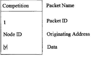
Figure 4.6: Competition packet model... 44

Figure 4.7: Update packet model...46

Figure 4.8: Organizational packet model... 47

Figure 4.9: Maintenance packet model... 49

Figure 4.10: Movement of a sensor node... 50

Figure 5.1: RSOM step response vs. a ...54

Figure 5.2: RSOM impulse response (7$ = 1.0, a = 0 .3 )... 55

Figure 5.3: Schematic picture of an RSOM filter (image taken from [35])...55

Figure 5.4: RSOM frequency response (TS = 1, a = 0 .3 )...56

Figure 5.5: Cutoff frequency vs. a ...57

Figure 5.6: Term weightings vs. a for N - 1 0... 58

Figure 6.1: Signal A ...62

Figure 6.2: Signal B...62

Figure 6.3: Neuron #1 activation (first 14 epochs)... 63

Figure 6.4: Neuron #2 activation (first 14 epochs)... 64

Figure 6.5: Neural response to noisy signal B (a = le-6 )...65

Figure 6.6: Neural response to noisy signal B (a = le-6 )...65

Figure 6.7: Total number of iterations vs. node population (inc. subplot magnification) 66 Figure 6.8: Number of neural collisions vs. iteration (150 nodes; incl. raw & smoothed)67 Figure 6.9: Neural collisions vs. iteration (160 nodes)... 68

Figure 6.10: (top) Neural collisions vs. iteration w/ deactivation (160 nodes)... 68

Figure 6.11: A trained RSOM (taken from [34])...70

Figure 6.12: Two-dimensional weight-vector gradient vs. topology... 71

Figure 6.13: Weight topology after node movement (no adjustment)...72

(11)

List of Abbreviations

ACE: Algorithm for Cluster Establishment ANN: Artificial Neural Network

CCR: Comer-Cube Retroreflector

DARPA: Defense Advanced Research Projects Agency DSN: Distributed Sensor Networks

DSR: Dynamic Source Routing

ESF: European Science Foundation

GAF: Geographically Adaptive Fidelity

HCP: Hexagonal Close-Packing

HEED: Hybrid Energy-Efficiency Distributed Clustering IPTO: Information Processing Techniques Office, DARPA LEACH: Low Energy Adaptive Clustering Hierarchy

MEMS: Micro Electromechanical Systems QoS: Quality of Service

RSOM: Recurrent Self-Organizing Map

SINA: Sensor Information Networking Architecture SNR: Signal-to-Noise Ratio

SOM: Self-Organizing Map

S OSUS: S ound Surveillance System

(12)

Chapter 1 Introduction

1.1 Wireless Sensor Networks

A wireless sensor network (WSN) is a wireless network consisting of low cost, low

power, multifunctional devices known as sensor nodes. Nodes are spatially distributed

within a region of interest, though their precise locations need not be engineered or

predetermined [1]. Node hardware typically includes a sensor, simple processing

elements, and a wireless transceiver that facilitates communication within a limited

radius. While the processing capability of each node is limited, the network benefits

from the high degree of aggregate parallel processing resulting from the collaborative

effort of many sensor nodes. WSNs have been identified as one of the most important

upcoming technologies that will change the world [3]. Potential and current applications

include inventory tracking [4], the monitoring of disaster areas [4, 5, 6], traffic control

[2], medical monitoring [7], space and planetary exploration [7] and military surveillance

[2, 4, 6],

Research leading to advances in wireless sensor network technology represents an

amalgam of research efforts in the fields of sensors, communications, and computing [2].

While isolated advancements in any of these fields subsequently leads to impetus in the

area of WSNs, as early as the late 1970s, research dedicated to the specific advancement

(13)

supported through funding. A principal benefactor of WSN research at this time was the

Defense Advanced Research Projects Agency (DARPA) through its Distributed Sensor

Networks (DSN) program [2].

1.1.1 Overview

Military applications have served as motivation for the research of many technologies,

including wireless sensor networks. WSN projects conducted mostly in the United Sates,

and specifically those by DARPA, shaped the early development of WSN research,

essentially establishing a de facto definition of a wireless sensor network as, “... a

large-scale ad hoc, multi-hop, unpartitioned network o f largely homogeneous, tiny,

resource-constrained, mostly immobile sensor nodes that would be randomly deployed in the area

o f interest. ” [8: pg. 1]. This characterization was based on the common goals of those

projects as well as the limitations of the technology of the period. However, as research

progressed and WSN technology evolved, this description became increasingly

inadequate [8], In 2004, the European Science Foundation (ESF) funded a workshop in

which experts gathered to discuss important WSN topics and to coordinate related

research activities in Europe. This workshop produced a more sophisticated scheme of

characterizing different types of wireless sensor networks based on several criteria;

deployment, mobility, form factor, heterogeneity, communication modality, network

topology, coverage, connectivity, network size, and other quality of service (QoS)

(14)

1.1.2 Deployment

The way in which sensor nodes are deployed will vary with application. The placement

of nodes may be random, or they may be deliberately placed in particular locations.

Nodes may also be imbedded within the target environment - for example, being mixed

into concrete or dropped into deep crevices, in which case they will subsequently be

inaccessible for maintenance or recovery (possibly bringing about environmental

concerns). Deployment may take the form of a one-time activity or may be an ongoing

process in which additional nodes are distributed to increase sensor density in interesting

regions or to take the place of old nodes that have become damaged, destroyed, or

otherwise ineffective [8]. Methods of deployment can be classified as: random vs.

manual; imbedded vs. accessible; one-time vs. iterative, and so on [see: 8].

1.1.3 Mobility

Following initial deployment, nodes may not remain in their original positions

indefinitely. Some network applications rely on the movement of nodes as an essential

phase of the sensing process. Sensing objectives that require the collection of data over a

very large region, such as an entire planetary surface, cannot be realistically achieved

with stationary nodes. A more practical solution is for each node to be mobile, so that

they can move to the next area of interest after the examination of their previous locations

have been completed. In this case, the mobility of nodes is a desirable feature of the

network. For other applications, the movement itself may be the matter under

(15)

Mobility can be achieved passively (the node is propelled by an autonomous entity), or

actively (under its own power and control).

1.1.4 Form factor

The physical configuration of a sensor node can take several forms, influenced by cost,

resource and size constraints. During the mid-1980s, the mobile nodes used in DARPA’s

DSN test bed had to be mounted to trucks due to their massive size and weight [2]. Since

that time, technological advancements have allowed the gradual miniaturization of sensor

nodes. Modem day research projects illustrate the reduction in scale that has become

achievable through Micro Electromechanical Systems (MEMS) fabrication techniques.

Researchers at University of California, Berkeley pursued a Smart Dust [9] project,

whose sensor nodes are no larger than a few cubic millimeters.

The untethered nature of sensor nodes precludes any connection to established

power grids. Nodes must therefore be entirely self-reliant on meeting their power

demands, either by scavenging energy from their environment (i.e. solar cells) or by

depleting an energy storage device such as a battery or fuel cell. Nodes that lack a

renewable energy supply have a maximum operational lifetime that scales with the

quantity of fuel at its disposal. In the case of battery-powered sensor nodes, lifetime is

therefore limited by the size of the battery, which may represent nearly the entire volume

(16)

1.1.5 Heterogeneity

There are two design paradigms regarding the level of conformity between sensor nodes

within a network. Homogeneous networks consist of nodes that are indistinguishable

from one another; both the hardware and software of these nodes are identical.

Homogeneous networks tend to be less expensive to manufacture due to the greater

degree of mass production of its nodes, and also more manageable to deploy since no

special attention is given to differing node species during placement. Conversely,

heterogeneous networks include more than one class of node, and attempt to optimize

available resources through the targeted deployment of specialized nodes to where they

are most useful. For example, a heterogeneous network may incorporate nodes

containing temperature and pressure sensors deployed to where both measurements are

necessary, and nodes with only pressure sensors deployed to regions where temperature

is unimportant. In contrast, a homogeneous network would be putting valuable

temperature sensing hardware to waste in the latter area. Heterogeneous networks may

require more sophisticated software than their homogeneous counterparts in order to

properly utilize the unique talents of each node.

1.1.6 Communication modality

Sensor nodes can exploit several modes of wireless communication, some being more

suited to particular environments than others. Ambient interference, line-of-sight

requirement, power usage, as well as the cost and complexity of the corresponding

transceiver hardware are the dominant considerations regarding the selection of a

(17)

the small size and low power of laser beam communication technology, despite its

reliance on there being line-of-sight between nodes. Possible methods of communication

include radio, light, sound, etc.

1.1.7 Network topology

The network topology of a WSN is a mapping of the wireless connections between

nodes. The simplest form of network topology (referred to as single-hop) arises when

every node is capable of direct communication with all others without the participation of

intermediaries. As circumstances that limit a node’s ability to establish wireless

connections arise, more complex topological patterns emerge. Topology is heavily

influenced by the mode of communication employed (which defines the maximum range

of connections as well as line-of-sight requirements), and also by infrastructure (which

may necessitate the channeling of messages through base stations). As the combinational

complexity of the mapping increases, the topology is typically characterized as a

combination of more basic topologies, each of which is determined by the configuration

of communicable nodes.

1.1.8 Coverage

The degree of coverage provided by a WSN is equivalent to how extensively an area is

monitored by sensors [8, 10]. Since each sensor has a limited range, a relationship exists

between the abundance of nodes employed and the level of coverage achieved. Coverage

can vary from sparse, where some coordinates lack monitoring, to dense, where every

(18)

same coordinate. In some cases, the level of coverage provided is neither spatially nor

temporally constant. A higher density of nodes may be deployed to the more interesting

regions of the monitored environment, and the movement of mobile nodes can alter the

degree of coverage over a period of time.

1.1.9 Connectivity

Connectivitycharacterizes a network’s resilience against fragmentation into two or more

isolated segments. The topology of a connectednetwork is such that a path exists

between any arbitrary pair of nodes, even if intermediate nodes are necessary for the path

to be established.

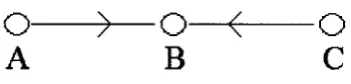
In Figure 1.1, three nodes form a connected network; starting at any node, a path

can be found that links it to the other two. Note that the directionality of the connections

is irrelevant when determining if the network is connected.

A network’s connectivityis a quantitative attribute, equal to the minimum number

of nodes that must be removed in order to create a partition in the network, thereby

causing it to be disconnected. When the removal of just one node causes a partition, the

network is referred to as being 1-connected. Networks can be described as 1-connected,

2-connected, n-connected, and so on. The topology shown in Figure 1.1 illustrates a

1-o

A

O

c

(19)

connected network, since the removal of a single node (node B) creates a partition

between nodes A and C, which lack an alternate communicable path.

Connectivity reflects the robustness of communication within the network. A

high level of connectivity may also bolster communication throughput by eliminating

bottlenecks [12]. Connectivity, like coverage, may need to be excessive at the time of

deployment, so that as nodes gradually die, connectivity will remain at a sufficient level.

The mobility of nodes in combination with a dynamic environment may cause

temporary disconnects. When these disconnects are occasional, the connectivity is said

to be intermittent [8]. However, as breaches in the network become more severe, and

partitions result in the isolation of nodes for most of the time, connectivity is referred to

as sporadic.

1.1.10 Energy management / lifetime

The maximization of sensor node lifetime goes hand-in-hand with the development of

energy management techniques. Recall that nodes tend to be energy-constrained devices,

therefore the lifetime of nodes cannot exceed that duration which the energy storage

mechanism can supply power. Whereas applications may require nodes to survive for

many years, special attention must be given to the issue of a node’s energy efficiency,

even when state-of-the-art batteries are being used.

1.1.10.1 Sleep scheduling

A common method to reduce the energy consumed by a network is to employ

(20)

rules. During the hibernating, sleep or idle periods, the node’s power usage is

significantly reduced, while simultaneously providing little or no services to the network.

To avoid interruption in the network’s operation, any load bom by a sleeping node must

be displaced to other active nodes. In general, nodes are expected to sleep when there is

little for them to do (such as when waiting for an incoming message), and the number of

nodes sleeping at any time reflects the quiescence of the environment. In sleep mode, a

node may turn off its radio [13], reduce power supply voltages [14], and so on.

1.1.11 Collaborative/distributed processing

Collaborative processing is an excellent feature for many distributed sensing

assignments. In many cases, the data collected by the sensing network is used as a basis

to form some control decision (i.e. the timing of traffic signals, the release of drugs into a

patient’s body, or alerting a human operator of an imminent tsunami). Though each node

has limited processing hardware, the dense placement of many nodes can produce enough

aggregate computational power to accomplish either the processing, or pre-processing of

their sensed data locally, before sending the results to a primary control center or

command station. The processing tasks can include pattern recognition, data

compression, and so on. Distributed processing sensor networks offer several advantages

over their sensing-only counterparts. A primary advantage is that local processing of data

has an effect of reducing the number of bytes that need to be transmitted to a control

station, thereby reducing communication power requirements. These energy savings are

(21)

processing power will scale with network size; therefore the number of nodes can be

adjusted to achieve an appropriate computational capability.

1.1.12 Other QoS requirements

The very wide range of applications seen by wireless sensor networks results in many

unique QoS design requirements. Military applications may require nodes to be

camouflaged, or entirely invisible (too small to be seen by the naked eye). Tamper-

resistance and eavesdropping-resistance, as well as physical robustness are other

considerations when designing individual nodes, as well as networking protocols.

1.2 Artificial Neural Networks

An artificial neural network (ANN) is a network of interconnected artificial neurons,

modeled after biological neural networks. Neurons perform simple processes on their

inputs, and forward their output along directional connections to other neurons. Since

many simple interactions between neurons leads to complex global behavior, most ANNs

systems give rise to emergent processes. Most ANNs are adaptive systems whose

structure changes during the learning phase, in order to achieve a processing objective.

1.2.1 Supervised learning neural networks

The structural parameters of a supervised-leaming neural network are updated during the

learning phase by being exposed to several input/output training pairs. The learning

(22)

them, within some small margin of error. To produce a training data set, a priori

information about the inputs must generally be known by an external supervisor.

1.2.2 Unsupervised learning neural networks

Unlike their supervised-leaming counterparts, unsupervised-leaming neural networks

have no a priorioutput, and no training data sets are used. Therefore, the only

information available to the network during learning is the inputs themselves. As a

result, unsupervised-leaming neural networks “evolve to extract features or regularities

in presented patterns, without being told what outputs or classes associated with the

input patterns are desired. ” [33: pg. 301]. Examples of unsupervised-leaming neural

networks include the Self-Organizing Map (SOM), Adaptive Resonance Theory (ART)

Network, and Hopfield Net.

1.2.2.1 The self-organizing map (SOM)

The self-organizing map (SOM) is a popular unsupervised-leaming neural network first

developed by Teuvo Kohonen in 1984, and is sometimes referred to as Kohonen’s self

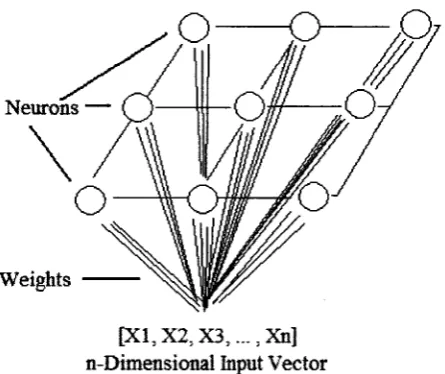
organizing map. An SOM is a dual-layer feed-forward neural network consisting of one

input layer and one output layer. Every neuron in the output layer is linked to the multi

(23)

Neurons —

Weights

[XI, X2, X 3 ,.... Xn] n-Dtmensional Input Vector

Figure 1.2: Self-organizing map structure

As shown in Figure 1.2, an n-dimensional input vector is connected to the output

layer of neurons. Each neuron is connected to the input layer by an n-dimensional weight

vector. Initially, each weight vector is set to small, random values. As inputs are

presented to the network, the weight vectors are modified to minimize a particular error

function. This has the effect of learning commonly encountered inputs. The SOM

weight-update formula is spatially dependent, so that similar inputs will be associated

with neurons in a small neighborhood, whereas very dissimilar inputs will be associated

with distant neurons in the map. An SOM is therefore also referred to as a

topology-preserving feature map.

1.3 Objectives

The objective of the research described in this thesis is to develop a simple, adaptive

architecture for wireless sensor networks that takes full advantage of the hardware’s

massive parallelism and redundancy. Simplicity is important to facilitate implementation

(24)

process of tailoring a network to a particular task. A related objective is the seamless

integration of a neural processing foundation with a wireless sensor network in order to

(25)

Chapter 2 Review of the State-of-the-Art

2.1 Themes in State-of-the-Art WSN Design

Issues related to the supply and consumption of power tend to dominate state-of-the-art

WSN research, due to the inaccessible and energy-constrained nature of sensor nodes.

While the development of superior batteries will certainly offer some relief to sensor

node designers, increasing the energy efficiency of nodes will be a continuing endeavor.

Wireless transceivers are the most exhausting components of sensor nodes, and most of

the energy wasted by the node is associated with wireless communication. Some

examples of energy waste in wireless communication include: re-transmission of lost or

corrupted data packets; transmitting data that is of no interest to the receiver; generating

communication signals that are stronger than is necessary to deliver data to its

destination; generating communication signals that flood an area much larger than what is

necessary to be received at the destination. The development of robust, multi-hop, self

organizing routing protocols is the objective of most WSN researchers as a mechanism to

reduce energy wasted in these ways.

2.1.1 Multi-hop communication

Multi-hop topologies rely on the forwarding of data from its source to its destination by

(26)

overhead associated with generating wireless signals. The energy invested in the

generation of an omni-directional signal scales with the square of the distance that the

signal must travel. Multi-hop communication is implemented by having several

intermediate nodes forward data, where each forwarding signal covers a fraction of the

total difference. Figure 2.1 and Figure 2.2 illustrate single-hop and multi-hop

communication strategies, respectively.

As shown in Figure 2.2, three signals are generated, each of which only needs to

Energy on order o f -2

o

r

Figure 2.1: Single-hop communication

Energy on order o f r for each signal 9

%

Figure 2.2: Multi-hop communication

(27)

Due to the exponential nature of omni-directional signal propagation, a collection of

several short-range signals represent a much smaller investment of energy than one long-

range signal. In the example shown in Figure 2.1 and Figure 2.2, the multi-hop strategy

requires only one-third the energy of the single-hop strategy to send a signal a total

distance of r.

2.1.2 Clustering

In many sensor network applications, sensor nodes are located close to each other, but far

from base stations. In terms of energy, local communication between nodes is almost

always less expensive than the long-distance communication between the nodes and the

base station. A very effective and commonly implemented method to achieve significant

energy savings is called clustering. Clustering is a category of network organization and

routing that reduces the amount of data transmitted long-range by aggregating, filtering,

and pre-processing data locally. Nodes must collaborate to decide which data warrants

the costly transmission to the base station; nodes must also collaboratively decide which

of them will generate the resultant transmission. Typically, the node aggregating the data

also sends the long-distance transmission and is responsible for coordinating cluster

activities. This node is referred to as the cluster-head, and the remaining cluster nodes

are referred to as member nodes. Typically, all member nodes are within a single-hop of

their cluster head, and are prohibited by the routing scheme from communicating with

member nodes of other clusters. In addition to communicating with base stations, it is

typical for cluster-heads to have the ability to communicate with each other. Cluster

(28)

cluster-head. A network that suffers from a large amount of cluster overlap tends to have a

higher number of total clusters, each of which has a low population. Many, low

population clusters tend to be less energy efficient when compared to having fewer large

population clusters.

2.2 Literature Review

University of California, Berkeley professors Kris Pister and Joe Kahn are the leaders of

the DARPA-supported Smart Dust project detailed in [9]. Smart Dust nodes (also

referred to as motes) were designed to have a volume no greater than one cubic

millimeter (“dust”-sized), while being equipped with hardware allowing for sensing, bi

directional communication, processing, and energy generation (see Figure 2.3). The

equipped solar panel was sufficient to allow for continuous power usage in the microwatt

(29)

R eceiv er with P h o to d e te c to r

Analog I/O, DSP, C ontrol S e n s o rs

P o w e r C ap acito r

Thick-Film Battery

Figure 2.3: A Smart Dust mote, with equipped hardware (taken from [9])

Pister and his team decided that their power targets could be realized if nodes

were spared the burden of generating their own communication signals. An innovative

infrastructure-based communications strategy was adopted, whereby a base station would

query nodes, and simultaneously supply the optical power needed by the nodes to

respond. A Comer Cube Retro-reflector (CCR) was incorporated into every node in

order to modulate and reflect a querying optical beam back to its originating base station

while requiring almost no investment of energy by the node. Unfortunately, this requires

a line-of-sight path between nodes and base stations, which need significantly more

available energy than nodes. Nodes are queried not by reference to a particular node

ID#, but rather spatially, since a given optical beam trajectory from the base station will

(30)

Shen et al. developed the Sensor Information Networking Architecture (SINA)

[17], which provides adaptive organization of sensor information, and facilitates query,

event monitoring and tasking capability. SINA utilizes attribute-based addressing,

whereby nodes are queried by the current states of several of their attributes, such as

general location and the value of their sensed data. In other words, instead of the

following address-based query, “Node #127, report your data”, the attribute-based query

may take the form, “To all nodes in the northwest region: reply if you are sensing a

temperature greater than 100 degrees Celsius”. SINA also provides clustering

components to facilitate organized scalability for very large networks. A cluster is

formed by collecting neighboring nodes, one of which (the cluster head) will take on

added responsibilities of coordinating the activities of the other nodes in the collective.

When appropriate, clusters themselves may be aggregated to form a cluster hierarchy.

In [4], Estrin et al. discuss the use of directed diffusion - a set of localized

algorithms, to accomplish networking goals, rather than using a centralized approach.

The authors describe localized algorithms as, “a distributed computation in which sensor

nodes only communicate with sensors within some neighborhood, yet the overall

computation achieves a desired global objective” [4: pg. 3]. It is proposed that compared

to a localized approach, a centralized one is a bad choice due to inadequate scalability,

energy inefficiency, and greater fragility. Their directed diffusion model is not based on

a sequence of queries and replies as in other strategies, but rather each node classifies its

particular attributes, and other nodes express some level of interest in those attributes. A

(31)

data from node to node. A node’s attributes may include its location, the type of data

being sensed (i.e. temperature, pressure, etc.), remaining energy supply, etc.

Shah and Rabaey also endorsed the idea that nodes’ power supplies should be

exhausted in a more uniform manner, and proposed an Energy Aware routing scheme in

[18]. The authors criticize energy-optimizing protocols that continually rely on an

optimal multi-hop path, since the available energy of the nodes in that path will be

rapidly depleted, “leaving the network with a wide disparity in the energy levels o f the

nodes, and eventually disconnected subnets” [18: pg. 1]. Instead, the energy-aware

protocols proposed by the authors are designed to maximize network survivability, as

they define it, by maintaining networking connectivity for as long as possible. In

accordance with their stated objective, Shah and Rabaey’s protocol alternates between a

set of good paths, rather than the continual reliance on an optimal path. It was shown by

the authors that their energy-aware protocols could extend network lifetime by up to 40%

over the directed diffusion scheme.

Low-Energy Adaptive Clustering Hierarchy (LEACH), described by Heinzelman

et al. in [19], is another localized, automated clustering architecture. The authors

recognized that the cluster-heads exhaust energy much more quickly than other nodes.

To more evenly distribute this energy burden, the cluster-head duties are often reassigned

to other nodes. The result is a more even depletion of energy supplies of all the nodes

across the network, leading to a more sudden, system-wide failure, rather than a gradual

crippling of the network due to an accumulation of individual node deaths over the

network’s entire lifetime. The former scenario is more desirable than the latter, since the

(32)

are reassigned in LEACH, the other nodes may also be reassigned to other clusters, since

the head of a different cluster may now be closer than the newly assigned cluster-head of

the old cluster. The authors used simulations to compare LEACH with static clustering

algorithms, and found that it took 8 times longer for the first node to die in LEACH as it

does with static clustering protocols, and 3 times longer for the last LEACH node to die

than the last node with static clustering protocols.

The Hybrid Energy-Efficiency Distributed Clustering (HEED) protocol described

by Younis & Fahmy in [20] is a clustering protocol designed to maximize the interval

between the network going online and the first node failure. The HEED protocol selects

cluster-heads randomly, where nodes with more residual energy are more likely to

become cluster-heads; cluster-head duties are re-assigned to other nodes at regular

intervals. When two potential cluster heads have equal residual energy, the one that is

associated with a lesser inter-cluster communication cost is selected. The authors

reported simulation results showing minor improvements in network lifetime over the

LEACH protocol.

Xu, Heidemann and Estrin described a Geographical Adaptive Fidelity (GAF)

algorithm in [21]. The term, “geographically adaptive” refers to GAF’s plotting of multi

hop paths between communicating nodes based on precise knowledge of their relative

positions, obtained through GPS or some equivalent system. Precise geographical

information can be used to ensure that the employed multi-hop path results in the least

amount of wasted energy compared to alternative paths. Nodes that are not participating

in the multi-hop path are powered down according to a sleep-scheduling algorithm. A

(33)

traffic areas do not become depleted as rapidly. The authors report that their GAF

algorithm consumes 40% to 60% less energy compared to DSR (Dynamic Source

Routing) [23, 22] and AODV (Ad Hoc On-Demand Distance Vector) [24, 22]. DSR and

AODV are similar protocols that were developed in the 1990s for ad hoc networking of

computers that are not subject to significant energy constraints (such as laptop

computers).

GS3 is a hexagonal close-packing (HCP) clustering algorithm presented by Zhang

and Arora in [25]. GS3 forms hexagonally shaped clusters starting a “big node” and

spreading outwardly until the entire network is covered. Big nodes are responsible for

initiating the clustering process and are the only nodes capable of communicating with

external systems including base stations or other computer networks such as the Internet.

In order to efficiently form hexagonal clusters with minimal overlap (overlap occurs

when the boundaries of adjacent clusters intersect), GS3 requires precise geographical

information about each node, and every node in the network must lie on the same two-

dimensional plane. GS3 produces excellent cluster uniformity and less cluster overlap

than competing clustering algorithms.

ACE (Algorithm for Cluster Establishment) is a clustering protocol reported by

Chan and Perrig in [26] that is designed to minimize cluster overlap (overlap occurs when

cluster boundaries intersect) while providing full cluster coverage. ACE is an emergent

algorithm that requires no centralized authority; execution of the ACE protocol only

requires nodes to communicate with neighbors within a single-hop range. ACE achieves

7

excellent population uniformity in clusters with very little overlap. Unlike GS , the ACE

(34)

reported in the literature show that in certain circumstances, the amount of overlap

generated by ACE could approach what is achievable with Hexagonal Close-Packing

algorithms such as GS3. Recall that GS3 is a honeycomb-packing algorithm that requires

precise geographic information of each node.

Chou et al. proposed a sophisticated distributed data compression strategy to

reduce communication energy in [27]. The authors suggest that there exists an inherent

correlation between the sensor data acquired by densely deployed sensor nodes. The

underlying correlation is the basis of consequent redundancy in the network’s collective

sensor data. In other words, the underlying premise of the authors’ work is that if

variable Y is known, and a correlation between X and Y is known, then X must only be

partially known in order to extract the fu ll value o fX as a result o f X ’s known

dependency on Y. In essence, the strategy requests that nodes transmit data that is

incomplete to varying degrees. A special “data-gathering” node can fill in the missing

pieces of data by analyzing all of the incomplete fragments that it has received, assuming

it knows how all of the fragments are correlated. Initially, no correlation is known, and

the data-gathering node requires sensor nodes to transmit their whole readings.

Correlation tracking algorithms are used by the data-gatherer to construct a correlation

table between nodes. As the correlation table becomes more complete, the data-gathering

node will instruct sensing nodes to transmit a smaller fraction of their data, and the

correlations will be used to extract the missing pieces. This heterogeneous scheme

allocates all of the intensive correlation-based computations to the data-gathering nodes.

The compression algorithm used by each sensor node is rudimentary, and consists of only

(35)

the proposed strategy is robust against errors, and tolerant of noise, while achieving

significant energy savings. The authors indicate that their proposed strategy can reduce

the communication energy expended by each sensor node by up to 65%.

Oldewurtle and Mahonen proposed the use of a two-level, hierarchical neural

network algorithm to achieve fault-tolerance, data compression and parallel processing in

[28]. In [28], each sensor node would run a software-based Hopfield Net as a way to pre-

process their locally collected sensor readings (the authors assumed two or more sensors

would be present in each node). It must be stressed that each sensor node does not

represent a neuron in a large Hopfield Net, but rather a virtual Hopfield Net consisting of

multiple neurons is fully implemented through software at each sensor node. For

example, if a sensor network consists of one hundred sensor nodes, each which has three

different sensors, then there would be one hundred Hopfield Nets; each Hopfield Net is

associated with a particular sensor node, and is used strictly to process the three-

dimensional sensor data df the sensor node on which it is being simulated. These local

Hopfield Nets form the first level of the neural network hierarchy in the literature. The

second level is implemented by sensor node cluster-heads. Each sensor node transmits

the output of its Hopfield Net to the cluster-head, which aggregates the data using a self

organizing map (SOM). The cluster-head uses a virtual SOM with 5x4 neurons to

perform an X-to-2 dimensionality reduction on the combined output of a cluster

containing X sensor nodes.

The work of Kulakov et al. in [29] is similar to Oldewurtle and Mahonen [28]. A

two-level hierarchy of neural networks is implemented on a WSN. Both levels of the

(36)

level, each sensor node simulates a Fuzzy ART neural network to classify only its own

sensor readings. The authors used real Smart-It sensor nodes to collect data. The Smart-

It node includes six different sensors, and the virtual FuzzyART running in the node’s

software classifies patterns that occur in the simultaneous readings of those six sensors.

The output of the FuzzyART at each node is transmitted and collected by a cluster-head.

The cluster-head runs the second-level of the hierarchy, which is a binary ART network

whose inputs are the FuzzyART outputs from each other node in the cluster. The

architecture self-organized well and showed robustness to sensor errors.

Caterall et al. investigated the use of sensor nodes to represent individual neurons

in a self-organizing map (SOM) in [30]. The physical hardware used in the author’s

experiment consisted of five Smart-It nodes, which each contain six different sensors. In

an effort to reduce communication overhead, the authors made a slight change to the

original SOM model. Recall that in a classic SOM (see Figure 1.2) a single input vector

is presented to each neuron. Consequently, the inpih vector seen by each neuron is

identical. If Caterall et al. adhered to the original SOM model, the input to each neuron

would be a thirty-dimensional vector (five nodes x six sensors each). However, each

node has only local access to its own six sensor readings, therefore the remaining twenty-

four inputs would need to be transmitted wirelessly. In other words, whenever a node

took sensor readings, it would need to wirelessly transmit that data to every other node.

The authors opted to modify the original SOM and arrived at the model illustrated in

(37)

SOM Neuron

Weight Vector

Figure 2.4: SOM model used in [30]

As shown in Figure 2.4, in the modified SOM model used by Caterall et al., each

of the five neurons acts on a unique six-dimensional input vector, which corresponds to

the six sensor readings that have been acquired locally by its six sensors. The assumption

made by the authors is that the sensor readings will only vary slightly from node to node.

As a result, each node’s six-dimensional input vector will not be exactly the same, but

will be very similar. Due to the SOM redesign employed, for every set of inputs, each

node must only transmit one small data packet to the rest of the network. The packet

includes an identification number belonging to the transmitting node, a timestamp, and

Euclidean error between the node’s weight and input vectors. Experimental results

showed that after training, the SOM neurons organized to classify sensor patterns.

Zindel developed a thesis [31] in which a supervised-leaming neural network

implementation of a WSN was used to track the shadows cast by clouds as they moved

across a field. Zindel’s implementation used recursive subtrees of feed-forward, back-

propagation neural networks. After training, the network achieved a high success rate of

(38)

about ninety-five percent depending on how many input/output pairs were used during

(39)

Chapter 3 The WSN Problem

3.1 Problem Statement

WSN networking and processing software must achieve energy-efficient, fault-tolerant

processing while simultaneously coping with node mobility and frequent node failures,

and provide sufficient flexibility to allow for deployment in a wide variety of

applications. For quick and easy deployment, detailed a priori knowledge of the target

environment should be unnecessary. In other words, WSNs should adapt to their

surroundings with minimal application-specific preprogramming and administrator

oversight. To accommodate arbitrary numbers of nodes, architectures should be fully

scaleable - the network should benefit from every additional node, and suffer equally

from each node disconnect. The parallel processing capability of WSNs should be robust

and versatile, suitable for deployment in a wide range of diverse applications. Since

many sensed phenomena are represented by time-domain signals (such as voice audio,

weather patterns, vibrations in machinery and so on), the WSN’s processing algorithms

should be sensitive to temporal patterns as well as spatial ones. With no a priori

knowledge of the target environment, and therefore little knowledge of the input vectors

that will be encountered, the WSNs must have the capability to recognize patterns and

generate outputs based on input patterns of arbitrary length. For example, a military

(40)

the target language is of different lengths, and therefore produce sequences with varying

numbers of terms.

3.2 Analysis of State-of-the-Art Solutions

When evaluating the state-of-the-art of WSN protocols, it helps to have a historical

context. While DARPA’s DSN program was underway in the early 1980s, Dr. Robert

Kahn was the director of the organization’s Information Processing Techniques Office

(IPTO). Dr. Kahn, a co-inventor of the TCP/IP protocol and a key figure in the

development of the Internet [2, 32], was interested in applying the same approach of

networking to sensor networks [2]. While this may have been a worthwhile endeavor

two and half decades ago, the quantum leap that has meanwhile occurred in computer

hardware technology allows for WSN networks whose performance requirements easily

overwhelm traditional packet-switching protocols. Researchers have directed attention

towards developing incremental changes to these protocols in the attempt to make them

better suited to WSN applications, and perhaps through this evolutionary process,

hereditary weaknesses are still evident in much of the current state-of-the-art.

Clustering algorithms in state-of-the-art architectures are intended to reorganize

the network into multiple subgroups, each of which is of a more manageable size. There

are, however, some drawbacks associated with the clustering algorithms employed by

state-of-the-art WSN architectures. The organization of the network into clusters is an

arduous task. For increased efficiency, clusters should be uniform in size and closely

packed with minimal overlap. Meeting these targets requires either an iterative

(41)

lies on a common two-dimensional plane (as in [25]), or that precise GPS information for

every node is available (as in [21 & 25]). Once formed, clusters are fragile entities that

are disintegrated by the death of the cluster-head, or as a result of their mobile

constituents wandering too far apart. Due to their delicate nature, re-clustering is an

ongoing process, with each repetition wasting time and energy. Therefore, clustering

algorithms are not particularly resilient to node failures, are unable to effectively cope

with node mobility, and require repeated energy expenditures in the form of overhead.

The most intrinsic quality of WSNs is their massive parallelism, which leads to a

natural synergy with a parallel approach of processing their collected data. Since

clustering itself does not lead to any inherent parallel processing capability, a second,

application-layer protocol is needed to exploit the network’s parallel hardware. Several

state-of-the-art architectures apply artificial neural network (ANN) algorithms to achieve

fault-tolerant parallel processing in sensor networks (for example, [28 - 31]). Neural

networks share many inherent and desired characteristics with wireless sensor networks,

such as relying on many simple local interactions to give rise to complex global behavior.

Neural network implementations of WSNs are gaining popularity and attention among

researchers [31], though several deficiencies are present in state-of-the-art neural WSN

architectures. Supervised-leaming ANNs (used in [31], for example) require a priori

knowledge of the target environment, in the form of many input/output training pattern

pairs. These input/output pairs must be crafted ahead of time by a human administrator

(even if the pairs were generated by a separate computer system, that computer would

(42)

None of the state-of-the-art ANN-WSN architectures [38 - 31] are temporally

sensitive. In other words, they can only perform a computational analysis based on the

spatial distribution of input values and are indifferent to the time at which the inputs are

occurring. As previously stated, these state-of-the-art protocols are incapable of

(43)

Chapter 4 RSOM-WSN Architecture

4.1 Introduction

The architecture proposed in this thesis is referred to by the rather unimaginative name

RSOM-WSN. RSOM-WSN is a neural-based architecture that is self-organizing, tolerant

to both data errors and communication faults, and requires no a priori information about

its environment. RSOM-WSN is also designed to recognize geographic and temporal

signals. In other words, data patterns can be recognized regardless of their spacio-

temporal locality. The underlying neural framework used is the Recurrent Self-

Organizing Map (RSOM), which has never before been implemented in a sensor network

setting. In RSOM-WSN, each sensor node acts as a neuron in an RSOM neural network,

and therefore hardware sensor nodes act as complete analogues to RSOM neurons.

4.2 The Recurrent Self-Organizing Map (RSOM)

4.2.1 Overview

The recurrent self-organizing map is a powerful variant of Kohonen’s original self

organizing map. First proposed by Varsta et al. in [34], the RSOM is a recurrent network

that generates outputs based on a sequence of input vectors, rather than on a single input

(44)

4.2.2 RSOM algorithm in detail

4.2.2.1 RSOM input space

The RSOM is a dual-layer recurrent neural network, in which there is one input layer and

one output layer. Input vectors originate at the input layer and are connected to each

neuron in the output layer by a weight vector whose dimensionality is equal to that of the

input vector. Each input vector sequence may be arbitrary in length, having N terms.

For example, suppose that a two-dimensional input sequence is as follows.

Dimension #1 —>(0.0, 0.5, 1.0, 1.5, 2.0, 2.5)

Dimension #2 —>(1.2,4.5, 6.1, 7.9, 8.1, 9.5)

N = 6 terms

In this example, the input sequence consists of six terms, where each term is a

two-dimensional input vector,

Input vector sequence —> [0.0, 1.2], [0.5, 4.5], [1.0, 6.1], [1.5, 7.9], [2.0, 8.1], [2.5, 9.5]

4.2.2.2 RSOM neuron output function

Each neuron in an RSOM neural network generates its own output, determined by a

recursive, iterative function that is re-evaluated as each input vector in the sequence is

(45)

y ( n ) = ( l - a ) y ( « - 1) + a (jc (/i) - w)

y(0)=o

Where,

y (n) is the neuron' s cumulative output after the nth term of the input vector sequence,

x (n) is the nlh term of the input vector sequence,

w is the neuron' s weight vector, 0 < a < 1 is a learning constant

y, x, and w vectors with the same dimensionality

Equation 1. RSOM recursive output function

The output function can be considered as a decay of the previous level of output, y

(n), with a simultaneous re-enforcement of output caused by the most recent input term, x

(n). Equation 1 can be re-written to explicitly show the contribution that each input term

has on the cumulative output.

F o ra sequence with N terms, let RSO M (x, w ,a ) = y (N — 1), where

y ( N - \ ) = a x ( N - 1) - w +(1 ( N - 2 ) - w ) +( l - a ) 2( * ( A f - 3 ) - w ) + . . . + ( l - a ) N ( 0 ) - w )

Equation 2. RSOM output function (expanded)

Equation 2 explicitly shows the contribution each input term has on the neuron’s

cumulative output, and the function RSOM(x, w, a) is defined as the cumulative output

after all N terms of the input sequence have been presented. Essentially, the RSOM

output function computes an exponentially weighted sum o f biased inputs. As shown in

Equation 2, each input vector term, x(n) is biased by w, which is a neuron-specific

modifiable parameter. Each biased input is then weighted such that the terms located

towards the end of the sequence are given more weight than terms located early in the

(46)

4.2.2.3 RSOM neuron competition and the BMU

After every term in an input sequence has been presented to the network, each neuron

computes an absolute output, lyl, which has a value equal to the magnitude of its output

vector, y. Neurons “compete” by comparing their absolute outputs with that of the rest of

the network. The neuron with the smallest absolute output wins the competition and is

referred to as the best matching unit, or BMU. The BMU represents the neuron whose

weights were most well trained with respect to the input sequence, that is, the neuron

whose weights resulted in the least amount of output.

4.2.2.4 RSOM neuron weight vector and learning rule

Each RSOM neuron is associated with its own modifiable parameter known as a weight

vector. The naming of this vector as a ‘weight’ by RSOM’s inventors is to maintain

some level of consistent terminology with other types of neural networks, and in this case

is somewhat misleading. The weight vector in an RSOM neuron is not participatory in

any multiplicative weighting, but rather serves as a bias or offset. Subsequently in this

thesis, the weight vector may be referred to as an offset, or biasing term.

Initially, the weight vectors of every neuron are random. This represents a fully

untrained state of the network, since no input sequences have yet been encountered. As

input sequences are encountered, the weight vectors of neurons are modified according to

(47)

wi( r + l ) = w i(0 + Aa (0 y,(t)

Where,

w (t) is the old weight vector, hib is a neighborhoodfunction, and y/j is the neuron' s output vector

Equation 3. RSOM Weight-update formula

The neighborhood function in Equation 3 is a function related to the distance

between neuron i and the BMU. In typical learning schemes, 0< = h <= 1, and h

produces its maximum value at the BMU, and decreasing values for every neuron at an

increasing distance from the BMU’s location. In other words, neurons near the BMU

(including the BMU itself) will modify their weights by greater amounts than neurons

that are farther away. The neighborhood function plays a key role in establishing the

RSOM’s topology-preserving characteristic.

A neuron’s weight vector is modified according to the update formula in such a

manner that if the same input sequence is encountered in the future, the corresponding

output, y, will decrease. In this sense, a neuron’s output, y, can be thought of as an error

or cost function that the weight-update formula is attempting to minimize. Therefore, a

neuron that has been fully trained to recognize a particular input sequence will produce

an output of y - 0 whenever that input sequence is encountered. The ideal value of w

(48)

N - 1

N - l - K

W =* = 0_{N -}₁

£ ( i - “ )

k= 0

where N is the number o f terms in sequence x

Equation 4. Analytical computation of ideal weight for sequence x

4.2.3 Interpretation

The RSOM function computes an exponentially weighted sum of biased inputs. Neurons

are trained to recognize common input sequences by finding a weight, w, which results in

the RSOM function producing a zero output. For illustrative purposes, consider the

following steps in computing an RSOM output (for the sake of simplicity, in the

following example the input sequence is assumed to be one-dimensional). Also recall

that the following computations are conducted by each neuron separately.

The first step of the RSOM neural algorithm is to offset the input sequence by the

neuron’s weight vector, w.

w = -2 4 3 2 1 0 1 -2 -3 -4 180 200 140 160

60 80 100 120

0 20 40

(49)

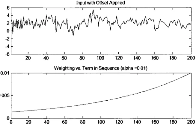
The second step is to multiply the biased input by an exponential curve whose

shape is determined by the parameter, a.

Input with Offset Applied

6

4

2

0

2

-4

-6

20 40 60 80 100 120 140 160 180 200

Weighting vs. Term in Sequence (alpha =0.01)

0.005

q _________i__________i_________ i_________ i__________i_________ t_________ i_________ i_________ i________

0 20 40 60 80 100 120 140 160 180 200

Figure 4.2: RSOM function step #2

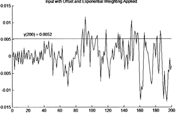
The third step is to sum the value of each term. Graphically, this equivalent to

(50)

0.015 r

Input with Offset a n d Exponential W eighting Applied

-0.005 0.005

-0.01 0.01

0

-0.015

0 20 40 60 80 100 120 140 160 180 200

Figure 4.3: RSOM function step #3

In Figure 4.3, it is shown how terms near the end of the sequence have been

amplified as a result of the exponential weighting performed in step 2. The RSOM

algorithm results in a high degree of data compression, since a multi-dimensional

sequence consisting ofynany terms is reduced to a single value, y.

RSOM-WSN sensor nodes are directly analogous to RSOM neurons. Therefore, the

number of neurons in the WSN-RSOM output layer is equal to the number of sensor

nodes in the WSN-RSOM network. Additionally, since sensors are providing the neural

inputs, and each node contains a sensor, every sensor in the network represents an

element in the RSOM’s input layer. Therefore, the dimensionality of the RSOM-WSN

input vector (as well as all weight vectors, w, and output vectors, y) is also equal to the

(51)

sensor). Therefore, an RSOM-WSN network with fifty sensor nodes acts on a fifty

dimensional input vector, and contains fifty neurons in its output layer. The RSOM-

WSN model is shown in Figure 4.4.

sensor nodes

input layer |

Figure 4.4: RSOM-WSN model with four sensor nodes

Typically, RSOM neural networks act on different input sequences that all have the

same number of terms. The number of terms is known before hand, and is either by

design or based on a priori knowledge of the input set. Wireless sensor networks, on the

other hand, which act on input vectors that can be largely unknown at the time of

deployment and also need the flexibility to operate in numerous applications, must have

the capability to recognize patterns and generate outputs based on input patterns of

arbitrary length. For example, a military surveillance network may be designed to

recognize human speech, though each word in the target language is of different lengths,

(52)

4.4 RSOM-WSN Protocols

The RSOM-WSN protocols proposed in this thesis serve as both networking and

processing protocols. Whereas most wireless sensor networks implement networking and

processing as separate layers (such as in TCP/IP), RSOM-WSN accomplishes both tasks

simultaneously with dual-function packets.

An innovation of RSOM-WSN is in its data transmission strategy. Rather than

using a query-reply strategy as seen in most state-of-the-art literature, RSOM-WSN

employs what this thesis refers to as a broadcast-react strategy. Unlike query-reply, in

which messages are directed to a specific destination, RSOM-WSN nodes merely

broadcast messages, without any specific recipient in mind and without intending to

respond to a query, or provoke a reply. The broadcasted messages flood the network, and

will elicit neural reactions in any node that receives the signal. Sensor nodes employing

the RSOM-WSN protocol are uncoordinated, largely unsynchronized, and completely

autonomous. RSOM-WSN nodes are reactionary because their behavior arises in

response to unscheduled stimuli. The protocol is a collection of event-driven processes

that maintain node autonomy while also achieving global, intelligent, fault-tolerant

pattern recognition. The wireless data packets that are broadcast from nodes are

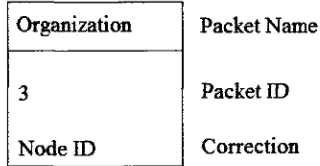
classified as one of three types, reflecting the purpose of the transmission. They are,

organizational, maintenance, and neural. Organizational packets ensure that each sensor

node possesses a unique node ID number, or address. Maintenance packets recalibrate

neural weight vectors when node movement distorts them, and neural packets include all

data necessary for input dissemination, weight updating, and ultimately pattern

(53)

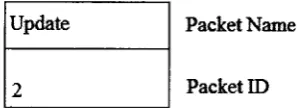
4.4.1 Neural packets

There are three kinds of neural packets, input, competition, and update, numbered as

packets 0 through 2, respectively. The broadcasting of any of these three packets from a

node requires a triggering event, and broadcasted packets trigger a reaction in all nodes

that receive them.

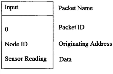
4.4.1.1 Input packets

Each node in RSOM-WSN performs a neural computation on a multi-dimensional input

vector. The dimensionality of this vector is equal to the number of nodes in the network,

and the value at each dimension corresponds to a sensor reading of a particular sensor

node. Therefore, every sensor node must share its sensor data with every other node in

the network. This data is transmitted in the input packet. Sensor nodes take regular

sensor samples at a sampling frequency, Fs. After a node takes a sample, it broadcasts an

input packet of the following form.

Packet Name

Packet ID

Originating Address

Data

Figure 4.5: Input packet model Input

0

Node ID

An adaptive, self-organizing, neural wireless sensor network.

Scholarship at UWindsor

Scholarship at UWindsor

An adaptive, self-organizing, neural wireless sensor network.

An adaptive, self-organizing, neural wireless sensor network.

Abstract

Dedication

Acknowledgements

Contents

List of Figures

List of Abbreviations

Chapter 1

Introduction

1.1 Wireless Sensor Networks

1.1.1 Overview

1.1.2 Deployment

1.1.3 Mobility

1.1.4 Form factor

1.1.5 Heterogeneity

1.1.6 Communication modality

1.1.7 Network topology

1.1.8 Coverage

1.1.9 Connectivity

1-o

A

O

c

1.1.10 Energy management / lifetime

1.1.10.1

Sleep scheduling

1.1.11 Collaborative/distributed processing

1.1.12 Other QoS requirements

1.2 Artificial Neural Networks

1.2.1 Supervised learning neural networks

1.2.2 Unsupervised learning neural networks

1.2.2.1 The self-organizing map (SOM)

1.3 Objectives

Chapter 2

Review of the State-of-the-Art

2.1 Themes in State-of-the-Art WSN Design

2.1.1 Multi-hop communication

o

2.1.2 Clustering

2.2 Literature Review

Chapter 3

The WSN Problem

3.1 Problem Statement

3.2 Analysis of State-of-the-Art Solutions

Chapter 4

RSOM-WSN Architecture

4.1 Introduction

4.2 The Recurrent Self-Organizing Map (RSOM)

4.2.1 Overview

4.2.2 RSOM algorithm in detail

4.2.2.1 RSOM input space

4.2.2.2 RSOM neuron output function

y(0)=o

4.2.2.3 RSOM neuron competition and the BMU

4.2.2.4 RSOM neuron weight vector and learning rule

£ ( i - “ )

4.2.3 Interpretation

4.4 RSOM-WSN Protocols

4.4.1 Neural packets

4.4.1.1 Input packets