INVESTIGATION
Novel Use of Derived Genotype Probabilities
to Discover Signi
fi
cant Dominance Effects
for Milk Production Traits in Dairy Cattle
Teide-Jens Boysen,*,1Claas Heuer,*,1Jens Tetens,*,2Fritz Reinhardt,†and Georg Thaller*
*Institute of Animal Breeding and Husbandry, Christian-Albrechts-University Kiel, D-24098 Kiel, Germany, and†Vereinigte
Informationssysteme Tierhaltung w.V., D-27283 Verden/Aller, Germany
ABSTRACTThe estimation of dominance effects requires the availability of direct phenotypes,i.e., genotypes and phenotypes in the same individuals. In dairy cattle, classical QTL mapping approaches are, however, relying on genotyped sires and daughter-based phenotypes like breeding values. Thus, dominance effects cannot be estimated. The number of dairy bulls genotyped for dense genome-wide marker panels is steadily increasing in the context of genomic selection schemes. The availability of genotyped cows is, however, limited. Within the current study, the genotypes of male ancestors were applied to the calculation of genotype proba-bilities in cows. Together with the cows’phenotypes, these probabilities were used to estimate dominance effects on a genome-wide scale. The impact of sample size, the depth of pedigree used in deriving genotype probabilities, the linkage disequilibrium between QTL and marker, the fraction of variance explained by the QTL, and the degree of dominance on the power to detect dominance were analyzed in simulation studies. The effect of relatedness among animals on the specificity of detection was addressed. Furthermore, the approach was applied to a real data set comprising 470,000 Holstein cows. To account for relatedness between animals a mixed-model two-step approach was used to adjust phenotypes based on an additive genetic relationship matrix. Thereby, considerable dominance effects were identified for important milk production traits. The approach might serve as a powerful tool to dissect the genetic architecture of performance and functional traits in dairy cattle.
I
N the context of genomic selection in dairy cattle, an abun-dance of bulls has been genotyped by applying genome-wide dense marker panels. In 2010, the European reference population comprised.17,000 bulls representing.20 mil-lion daughters (Lundet al.2010; Liuet al.2011). In addi-tion to their utilizaaddi-tion in genomic predicaddi-tion, these data are extensively used in genome-wide association studies to un-ravel the genetic factors affecting performance and func-tional traits. The expression of these traits is naturally limited to female individuals and thus, the phenotypes used in association studies are usually breeding values of sires based on performance data of many daughters. Such a struc-ture of data allows only the estimation of allele substitutioneffects. There is no direct possibility to distinguish between additive and dominance effects. For the detection of these allelic interactions, genotypes and phenotypes had to be known in the same individuals. Compared to the bulls, the availability of genotype data for cows is limited. With the increasing number of genotyped bulls, genotypes of male ancestors become available for many cows, enabling the derivation of genotype probabilities. Within the current study, these probabilities were converted to additive and dominance coefficients suitable for regression analysis anal-ogous to the procedures commonly applied to QTL mapping in resource populations (Haley and Knott 1992). The deri-vation of coefficients is not applied to intermarker intervals based on recombination fractions, but to unknown geno-types at given SNP marker positions. At a specific marker locus with two allelesAandB, the probabilities of the pos-sible genotypes AA, AB, and BB can be deduced in cows based on the male ancestor’s genotypes and the allele frequencies in the population. The approach implies a loss of statistical power compared to the utilization of real genotype data. A large number of genotyped bulls and an Copyright © 2013 by the Genetics Society of America
doi: 10.1534/genetics.112.144535
Manuscript received August 1, 2012; accepted for publication November 8, 2012 Supporting information is available online athttp://www.genetics.org/lookup/suppl/ doi:10.1534/genetics.112.144535/-/DC1.
1These authors contributed equally to this work.
2Corresponding author: Institute of Animal Breeding and Husbandry,
extensive number of daughters per sire, however, should compensate for these limitations.
Alternative methods to deduce genotype probabilities include “peeling” algorithms based on the ideas of Elston and Stewart (1971), Monte Carlo methods (e.g., Guo and Thompson 1992; Henshall and Tier 2003), or Bayesian approaches. These methods are computationally infeasible for the very large data sets as used within the current study. Approaches to impute genotypes based on phase informa-tion are inapplicable because this would require at least partly genotyped females. We conducted a series of simula-tion studies to discover both the capabilities and limitasimula-tions of the method and to evaluate the importance of factors like allele frequencies, sample size, and size of daughter groups. Subsequently, the approach was validated in a large German Holstein data set. The method presented herein enhances the utilization of existing large data sets to dissect the ge-netic architecture of important performance and functional traits in dairy cattle.
Materials and Methods
Derivation of genotype probabilities
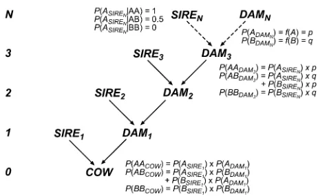
To calculate the three genotype probabilitiesPðAAÞ,PðABÞ, andPðBBÞfor a biallelic SNP marker with two allelesAand Band the respective allele frequenciespandqin a cow, we considered pedigrees including at least a genotyped sire and a maternal grandsire (Figure 1). For any genotyped bull, the probability to transmit allele Ais PðAÞ ¼1 in the homozygous ðAAÞ, PðAÞ ¼0:5 for the heterozygous ðABÞ, and PðAÞ ¼0 for the alternative homozygous state ðBBÞ. The probability to transmit allele B is PðBÞ ¼12PðAÞ. This information is unavailable for the female individuals. Therefore, the respective population frequency of the allele was used as an approximation for the transmission proba-bility from the maternal granddam to the dam of the cow under consideration. The genotype probabilities for the dam,PDðAA;AB;BBÞare the conditional probabilities emerg-ing from this approximation and the known genotypes of the maternal grandsires as summarized in Table 1. The allele frequencies were estimated from the bull data set, assuming that the allele frequencies in the cows are not considerably different from those observed in the bulls. For a given cow, nine possible scenarios exist, conditional on the genotypes of the sire and the maternal grandsire (Table 2). The respec-tive genotype probabilities can be calculated once and assigned to the cows by looking up the precalculated values. However, based on the genotype probabilities presented in Table 1, the transmission probability for allele A of the dam conditional on the genotype of the maternal grandsire, PðADjGTGSÞcan be calculated as the sum of the probability of being homozygous AA and half the probability of being heterozygous:
PðADjAAGSÞ ¼pþq
2¼ 2p
2 þ 12p
2 ¼
pþ1 2 ;
PðADjABGSÞ ¼
p 2þ
1 4¼
2p 4 þ
1 4¼
1þ2p
4 ¼
pþ0:5
2 ;
PðADjBBGSÞ ¼
p 2¼
pþ0 2 :
The second summand within the numerator in this case is equivalent to the transmission probability of the maternal grandsire, PðAGSÞ. Thus, the three equations can be jointly expressed as
PðADÞ ¼
1 2pþ
1 2PðAGSÞ:
Equivalently, the transmission probability for alleleB,PðBDÞ can be calculated as
PðBDÞ ¼
1 2qþ
1 2PðBGSÞ:
The probabilities for the homozygous genotypes in the cow arefinally calculated from the sire’s and dam’s transmission probabilities as follows:
PðAACowÞ ¼PðASÞ PðADÞ ¼PðASÞ
1 2pþ
1 2PðAGSÞ
;
Figure 1 Graphical representation of the pedigree structure used in the
calculation of genotype probabilities.Ndetermines the generation in
re-lation to the cow under consideration as used in the formulas to derive
probabilities.P(Genotype) with genotypesAA,AB, andBBis the genotype
probability andP(Allele) with allelesAandBis the transmission probability
for the respective allele.
Table 1 Genotype probabilities for the dam of the cow under consideration
Genotype GS PðAÞGS PðAAÞD PðABÞD PðBBÞD
AA 1 p q 0
AB 1
2
p 2
1 2
q 2
BB 0 0 p q
The probabilities were calculated from the allele frequenciesfðAÞ ¼pandfðBÞ ¼q
PðBBCowÞ ¼PðBSÞ PðBDÞ ¼PðBSÞ
1 2qþ
1 2PðBGSÞ
:
The probability of being heterozygous is simply calculated as PðABCowÞ ¼12PðAACowÞ2PðBBCowÞ. It is also possible to directly calculate the cow’s probability of being heterozy-gous as
PðABCowÞ ¼PðASÞ PðBDÞ þPðBSÞ PðADÞ:
Referring to Table 1 and considering the example of a sire with genotypeAAand a maternal grandsire with genotype BB, the probability can be calculated as
PðABCowjGTS¼AA;GTGS¼BBÞ ¼PðASjGTS¼AAÞ PðBDjGTGS¼BBÞ
þ PðBSjGTS¼AAÞ PðADjGTGS¼BBÞ
¼1
qþ1 2p
þ01 2p¼qþ
1
2p¼12pþ 1
2p¼12 1 2p
(see Table 2).
This calculation would allow distinguishing between dif-ferent parental origins of the alleles, resulting in the two probabilities PðApatBmatÞ and PðBpatAmatÞ, which could be used to analyze imprinting effects. This was, however, out of the scope of the current study.
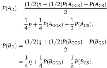
For practical reasons, all calculations were based only on the paternal transmission probabilityPðASÞand the frequency of the rare allelefðAÞ ¼prepresenting the minor allele fre-quency (MAF). PðBSÞ and fðBÞ ¼q were thus replaced by 12PðASÞ and 12p, respectively. The approach can readily be adapted for deeper pedigrees. With the inclusion of a gen-otyped maternal great-grandsire (GGS),i.e., three ancestral generations, the probabilities for the homozygous genotypes of the cow under consideration can be calculated similarly to the procedure described above. The transmission probabili-ties in the granddam are PðAGDÞ ¼12pþ
1
2PðAGGSÞ and PðBGDÞ ¼12qþ
1
2PðBGGSÞ. Multiplication by the transmission probabilities of the grandsire gives the genotype probabilities
of the dam, which can then be used to calculate the trans-mission probabilities. Analogous to the initial approach with two ancestral generations, the probabilities are
PðADÞ ¼ð
1=2Þpþ ð1=2ÞPðAGGSÞ þPðAGSÞ
2
¼1
4pþ 1
4PðAGGSÞ þ 1 2PðAGSÞ;
PðBDÞ ¼ð
1=2Þqþ ð1=2ÞPðBGGSÞ þPðBGSÞ
2
¼1
4qþ 1
4PðBGGSÞ þ 1 2PðBGSÞ:
Thus, the probabilities for the homozygous genotypes in the cow under consideration can be calculated as
PðAACowÞ ¼PðASÞ PðADÞ ¼PðASÞ
1 4pþ
1
4PðAGGSÞ þ 1 2PðAGSÞ
;
PðBBCowÞ ¼PðBSÞ PðBDÞ ¼PðBSÞ
1 4qþ
1
4PðBGGSÞ þ 1 2PðBGSÞ
:
The inclusion of a further generation (great-great-grandsire, GGGS) consequently leads to the following transmission probabilities in the dam:
PðADÞ ¼1
8pþ 1
8PðAGGGSÞ þ 1
4PðAGGSÞ þ 1 2PðAGSÞ;
PðBDÞ ¼
1 8qþ
1
8PðBGGGSÞ þ 1
4PðBGGSÞ þ 1 2PðBGSÞ:
To generalize the approach for any numberNof ancestral generations, the generations were numbered such that the cow under consideration represents generation “0”(Figure 1). The parents of the cow are generation 1 (SIRE1, sire; and DAM1, dam), the maternal grandparents are generation 2 [SIRE2, grandsire (GS); and DAM2], and the parents of DAM2are generation 3. DefiningNas the number of ancestral Table 2 Conditional genotype probabilities of a cow
Genotype sire
Genotype maternal grandsire AA AB BB
AA PðAAcowÞ ¼0:5þ0:5p PðAAcowÞ ¼0:25þ0:25p PðAAcowÞ ¼0
PðABcowÞ ¼0:520:5p PðABcowÞ ¼0:5 PðABcowÞ ¼0:5þ0:5p
PðBBcowÞ ¼0 PðBBcowÞ ¼0:2520:25p PðBBcowÞ ¼0:520:5p
AB PðAAcowÞ ¼0:25þ0:5p PðAAcowÞ ¼0:125þ0:25p PðAAcowÞ ¼0
PðABcowÞ ¼0:7520:5p PðABcowÞ ¼0:5 PðABcowÞ ¼0:25þ0:5p
PðBBcowÞ ¼0 PðBBcowÞ ¼0:37520:25p PðBBcowÞ ¼0:7520:5p
BB PðAAcowÞ ¼0:5p PðAAcowÞ ¼0:25p PðAAcowÞ ¼0
PðABcowÞ ¼120:5p PðABcowÞ ¼0:5 PðABcowÞ ¼0:5p
generations, the genotype probabilities can be calculated as follows:
PðAACOWÞ ¼PðASIRE1Þ 1 2N21pþ
XN
i¼2
1 2N2iþ1P
ASIREN2iþ2 !
;
PðBBCOWÞ ¼PðBSIRE1Þ 1 2N21qþ
XN
i¼2
1 2N2iþ1P
BSIREN2iþ2 !
:
The probabilities were transformed to regressors for addi-tive and dominance effects with add ¼PðAAÞ PðBBÞand dom ¼PðABÞ, which can be used in a simple linear regres-sion model of the form
yi¼mþb1addiþb2domiþei;
wheremis the mean,yirepresents the phenotype of theith animal, addiand domiare the additive and dominance
coef-ficients calculated from the genotype probabilities, b1 and
b2are the respective regression coefficients, andeiis a ran-dom residual term witheeNð0;s2
eÞ.
Simulation studies
To verify the functionality of our approach and to determine the necessary sample size to sufficiently detect dominance effects, populations of completely unrelated cows were sim-ulated. This was achieved by assigning an individual sire and grandsire per cow exclusively. A single biallelic marker in complete linkage disequilibrium (LD) with a nearby QTL was simulated. The sire genotypes for that marker were sampled from a population in Hardy–Weinberg equilibrium, given a MAF of 0.3. By utilizing the presented method for deriving genotype probabilities, the two coefficients add and dom were calculated for each cow based on the geno-types of sire, damsire, and the allele frequency. Furthermore, we assigned a true genotype for every cow by sampling genotypes given the probabilities presented in Table 2. This “true”genotype was used as a reference for the assignment of genetic effects to the simulated QTL. Phenotypes were calculated by assuming a defined phenotypic variance mul-tiplied by a given heritability of h2 = 0.25, leading to the additive genetic variance. The sizes of the simulated QTL effects were determined as a multiple of the additive genetic standard deviations (sA), with the additive effect being a half of the genetic standard deviation and the dominance effect making up half the size of the additive effect. Finally, a random residual effect was assigned to every phenotype.
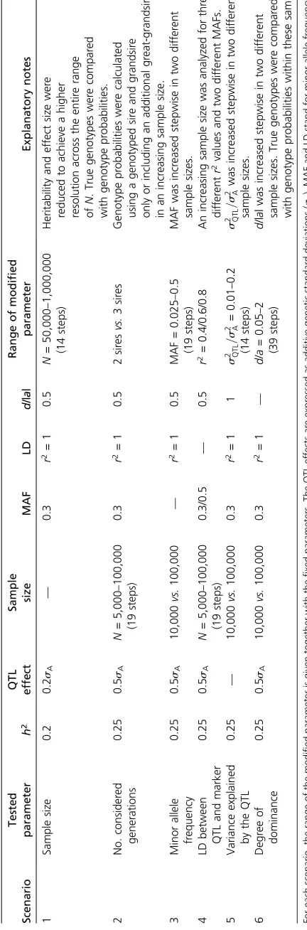
Subsequently, the influence of various properties of the created population and of the features of the simulated QTL on the power of detection was tested by separately varying the sample size, the number of considered generations, the minor allele frequency, the LD between QTL and marker, the fraction of variance explained by the QTL, and the degree of dominance. The effect of sample size was analyzed by a stepwise increase of up to 106cows. To achieve a better
resolution across the entire range ofN, a reduced heritability of 0.2 and a smaller QTL effect of 0.2 additive genetic stan-dard deviations were applied. The latter scenario was car-ried out with true genotypes as well as with genotype probabilities. The different scenarios are described in Table 3. For each scenario, 1000 iterations were performed and the power was defined as the rate of positives in the total number of iterations. The significance criterion wasfixed to 5% probability of error after a Bonferroni correction to ac-count for multiple testing. For this correction, 40,000 infor-mative markers were assumed, which is a realistic scenario for the application of the Illumina 50k SNP Chip in Holstein cattle (see,e.g., Habieret al.2010).
A second set of simulations was conducted to determine the influence of relatedness among animals and resulting stratification, which might lead to a high rate of false-positive signals. To this end, we repeated the simulations in a multimarker scenario including related ancestors of the cows. A sample of 100,000 cows was created, descending from initially 100 sires and 100 maternal grandsires. The phenotypes of the cows were assumed to consist of the combination of marker effects and additional polygenic ef-fects received from the ancestors. A trait of midrange heritability (h2= 0.3) was simulated with the genetic var-iance in the cows equally explained by the bull’s breeding values and the marker effects. The sires contributed half and the maternal grandsires one-quarter of their respective breeding values. A total of 150 markers with minor allele frequencies ranging from 0.05 to 0.5 were defined. One-tenth of the variance explained by markers was equally assigned to 10 of the markers, therefore each simulating a strong QTL. The dominance ratio was randomly assigned within these 10 markers. The remainder of markers was left without any effect. Subsequently, the effect of a varying fam-ily size was tested. For this purpose, the number of descend-ants per sire was varied from 50 to 5000 daughters, leading to different proportions of cows with identical sires and ma-ternal grandsires, thus representing groups of animals with uniform genotype probabilities. For each family size, the specificity was calculated as the number of true negatives divided by the sum of true negatives and false positives.
To correct for relationship among animals as a source of stratification, especially due to sires with a very large number of daughters, a single-marker linear mixed-model regression using residual maximum likelihood (REML) was applied. Therefore, a relationship matrix based on dam, sire, and damsire was used with the model
y¼XbþZaþe;
where y is a vector of phenotypes, b is a vector of fixed effects consisting of the intercept and the coefficients add and dom, andXis the incidence matrix for thefixed effects. The vectorarepresents the random effects withaeNð0;As2
residuals witheeNð0;Is2
eÞ, withIrepresenting an identity matrix. To test for significance, a Waldt-test was applied, where the denumerator degrees of freedom were numeri-cally estimated (Kenward and Roger 1997).
Application to a real data set
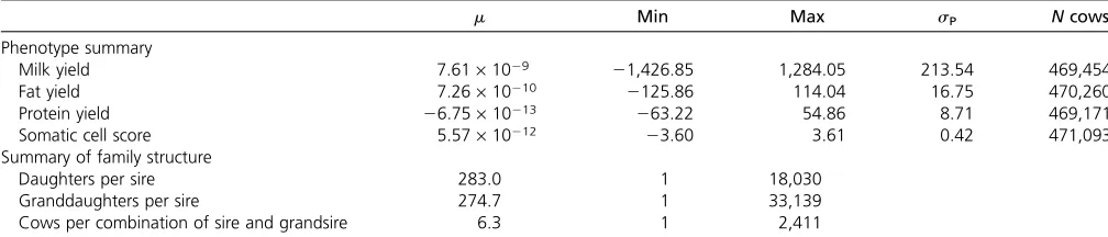
To validate the procedures with real data, phenotypic and pedigree data of 847,000 German Holstein cows were ob-tained from the Vereinigte Informationssysteme Tierhaltung w.V. (VIT). The phenotypic data consisted of yield devia-tions (YDs) for the traits milk, protein, and fat yield as well as somatic cell score (SCS) in thefirst lactation representing the deviations of the cow’s yields from the population mean adjusted for nongeneticfixed and random effects. The phe-notypic data are summarized in Table 4. Genotype informa-tion was available for 3200 Holstein bulls, genotyped with the Illumina BovineSNP50 BeadChip (Illumina, San Diego), featuring a total of 54,001 SNPs. The genotyping was done in the context of the GenoTrack research program funded by the German Federal Ministry of Education and Research. SNPs werefiltered for their minor allele frequency and miss-ing genotypes per locus. The thresholds were set to 0.05 and 0.1, respectively. Based on available pedigree information, a sample of 470,000 cows per trait with complete pheno-typic data and genotyped sires and maternal grandsires was assembled (Table 4). The cows descend from 2081 bulls of which 1916 occur as sire and 1981 as grandsire. A total of 86,254 unique sire–damsire combinations were observed. The data set consisting of the bull’s genotypes, the pedigree, and the yield deviation of the cows is available inSupporting Information,File S2. For this sample, the add and dom coeffi -cients were calculated according to the procedure developed within this study and phenotypes were regressed onto the coefficients by applying a simple linear regression model as outlined above.
Furthermore, the mixed-model approach as described above was applied to correct for family-based stratification. This approach is computationally challenging on a genome-wide scale. Thus, a two-step approach was applied, which is equivalent to the previously described genome-wide rapid association using mixed model and regression (GRAMMAR) approach (Aulchenko et al. 2007). It offers a way to effi -ciently reduce the time-consuming computations required for extensive pedigrees. In the first step, phenotypes were adjusted for a polygenic effect by applying the mixed model, but omitting the effects for add and dom. The residuals coming from this step were used as phenotypes in a subse-quent linear regression. With this two-step approach, the traits SCS, milk yield (MY), fat yield (FY), and protein yield (PY) were analyzed on a genome-wide scale.
To validate the two-step approach, chromosome 14 (BTA14) was analyzed by applying the full linear mixed model including a polygenic term as well as the coefficients for add and dom. BTA14 was chosen for this purpose, because the centromeric region of this chromosome contains a major QTL for milk production traits caused by polymorphisms in the
acylCoA-diacylglycerol-acyltransferase (DGAT1) gene (Riquet et al.1999; Grisart et al.2002; Spelmanet al.2002; Winter et al.2002; Thalleret al.2003; Welleret al.2003). This QTL segregates within the analyzed population and was thus used as a reference to evaluate the two-step approach as com-pared to a full model. Furthermore, those SNPs considered as genome-wide significant at a threshold ofP#0.01 after Bonferroni correction were reanalyzed by applying a full model including a polygenic effect and the coefficients for add and dom at the same time.
Implementation
All data-handling procedures including genotype integrity checks, recoding, and allele frequency calculation were per-formed using unix shell scripts together with the genome analysis toolsetplink(Purcellet al.2007). The derivation of genotype probabilities and simulation routines as well as regression models and test statistics were realized using the R statistical environment (R Development Core Team 2008). The R-script with the simulation routines as well as the R- and Shell-scripts used for data analysis can be found inFile S1. The linear mixed models werefitted using REML as implemented in ASReml 3.0 (VSN International) (Gilmour et al.1995).
Results and Discussion
Simulations
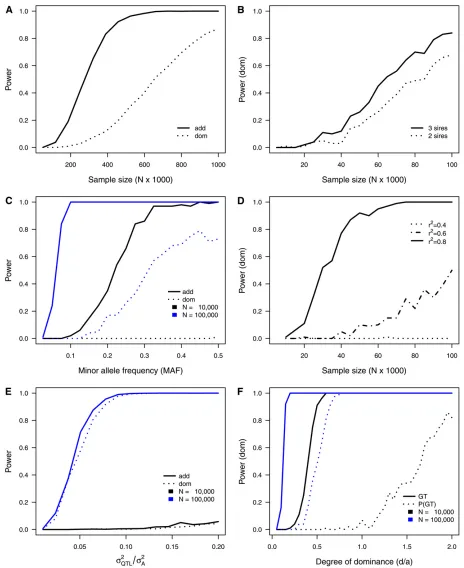
The results of the single-marker simulation scenarios are summarized in Figure 2, illustrating the major impacts on the power to detect additive and dominance effects, using genotype probabilities. All parameters under consideration substantially influenced the power of detection. Under a sce-nario with a heritability of 0.2 and an effect size of 0.2sA with d/|a| = 0.5 (scenario 1, Table 3), a sample size of 800,000 cows was needed to achieve a power of 0.7 for the detection of dominance effects (Figure 2A). With an effect size of 0.5sAand a heritability of 0.25 the same power can be achieved with 100,000 animals (Figure 2B). Approx-imately half of the sample size is needed to detect the cor-responding additive effects (Figure 2A). When using the true genotypes, powers of 0.94 and 0.69 for additive and
dominance effects, respectively, are achieved with 50,000 cows. A sample size of100,000 animals results in a power of 1 for both effects under these assumptions (not shown in Figure 2). Using genotype probabilities, the necessary sam-ple size is 10 times as large as needed with real genotype data. This clearly reflects the decrease in power arising from the impreciseness of genotype probabilities and the need to compensate this with a larger sample size. Under realistic conditions the power is even lower, because the simulated marker was assumed to be in complete LD with the QTL and the MAF wasfixed to 0.3. From Figure 2D it arises that with the reduction of r2 from 0.8 to 0.6 the power to detect dominance effects drops from 1 to 0.5 (scenario 4, Table 3) when assuming a MAF of 0.5. This scenario was also carried out using the standard MAF of 0.3, but the power was considerably lower (not shown in Figure 2D). The sub-stantial dependency between power and LD is reflecting the fact that only parts of the QTL variance can be explained by markers in incomplete LD. A marker showing an LD ofr2= 0.5 can capture approximately half of the QTL effect, mean-ing that the sample size must be doubled to capture an effect of a given size. Regarding the MAF, it can be seen from Figure 2C that a frequency of 0.5 results in the highest power to detect dominance effects (scenario 3, Table 3). This ideal situation cannot be expected under practical con-ditions. Thus, we set the MAF to 0.3 in the other simula-tions. For the additive effect, the MAF is not a limiting factor as in a sample of 100,000 cows the power equals 1 even for a MAF of 0.1. However, there might be a limitation to the strong interdependency between MAF and LD shown above. When there is incomplete LD between QTL and marker, the results are very sensitive to low minor allele frequencies. This has to be elucidated in further studies.
Another important parameter is the proportion of vari-ance explained by the QTL (scenario 5, Table 3). For a given degree of dominance ofd/|a|= 1, a QTL explaining5% of the additive genetic variance would be detectable with a power of 0.6 in a sample of 100,000 cows (Figure 2E). Assuming a heritability of 0.25, this would correspond to 1.25% of the phenotypic variance. That is a realistic value in dairy cattle (Hayes and Goddard 2001; Khatkar et al. 2004), leading to the conclusion that the approach should work well even for QTL with smaller effects. The power Table 4 Description of the real data set
m Min Max sP Ncows
Phenotype summary
Milk yield 7.61·1029 21,426.85 1,284.05 213.54 469,454
Fat yield 7.26·10210 2125.86 114.04 16.75 470,260
Protein yield 26.75·10213 263.22 54.86 8.71 469,171
Somatic cell score 5.57·10212 23.60 3.61 0.42 471,093
Summary of family structure
Daughters per sire 283.0 1 18,030
Granddaughters per sire 274.7 1 33,139
Cows per combination of sire and grandsire 6.3 1 2,411
The top section summarizes the mean (m), minimum (min), and maximum (max) values of the YD as well as their respective standard deviation (sP) and the number of cows
Figure 2 Graphical representation of the results obtained from single-marker simulation scenarios according to Table 3. (A) Power to detect additive (add) and dominance (dom) effects conditional on sample size (scenario 1). (B) Power to detect dominance effects conditional on sample size and the number of sires used in calculating genotype probabilities (scenario 2). (C) Power to detect additive (add) and dominance (dom) effects conditional on the minor allele frequency (MAF) in two different sample sizes (scenario 3). (D) Power to detect dominance effects conditional on sample size assuming
different LD (r2) between marker and QTL (scenario 4). (E) Power to detect additive (add) and dominance (dom) effects conditional on the proportion of
additive genetic variance explained by the QTL (s2QTL=s2
A) in two different sample sizes (scenario 5). (F) Power to detect dominance effects conditional on
curves for additive and dominance effects as shown in Fig-ure 2E are congruent, because the degree of dominance was set to 1. Figure 2F shows the dependency of the power to detect dominance under different degrees of dominance for a given total QTL effect (scenario 6, Table 3). From Figure 2 it can be seen that genotype probabilities calculated for a sample of 100,000 cows are sufficient to detect a degree of dominance of 0.33 at the given total QTL effect with a power of 0.8. Regarding the sample sizes discussed above, the detection of dominance effects even at a low de-gree of dominance is possible with the approach. Further-more, Figure 2F impressively illustrates the inferiority of genotype probabilities in small sample sizes. In a sample of 10,000 cows, a power of 1 can be achieved at d/|a| = 1 with true genotypes, while the application of genotype probabilities results in a power close to zero for thisd/|a|. A part of the decrease in power arising from the use of genotype probabilities can be compensated by the utilization of deeper pedigrees in the estimation of these probabilities. When usingNancestral generations, a proportion of 1=2Nof the available information arises from the allele frequency and is thus equal for all animals. With the inclusion of two ancestral generations, i.e., a genotyped sire and damsire, one-quarter of the information comes from the allele fre-quency. When including a genotyped great-grandsire, only one-eighth arises from the frequency. Figure 2B illustrates the impact of twovs.three genotyped male ancestors on the power to detect dominance effects, reflecting this depen-dency (scenario 2, Table 3). The inclusion of the third sire increases the power by 0.1 and 0.16 for 50,000 and 100,000 cows, respectively.
From the results of these single-marker simulation sce-narios it can be concluded that for traits of midrange her-itability, at least strong QTL effects can be detected with markers being in LD with the QTL in the range ofr2.0.4. However, the necessary sample size for detecting dominance effects is substantially.100,000 cows. A reliable power to detect smaller dominance effects might under practical con-ditions even require a sample size of.1,000,000 cows. This is, however, not limiting. Phenotypic data sets of this size are available on the basis of national evaluation and increasing reference samples in genomic selection schemes provide the necessary genotypic information. Furthermore, the simple regression approach presented herein is computationally not challenging. In reality, however, the finite number of sire–damsire combinations, representing the source of infor-mation for the genotype probabilities, will be the limiting factor in the sense of information content.
The second simulation was conducted as a multimarker scenario and focused on a more realistic population with family-based stratification. Expectedly, this led to the occur-rence of false positives in addition to those arising at random as type I error. This is reflected by the specificity to detect dominance as depicted in Figure 3. When increasing the number of daughters per sire from 50 to 5000, the specificity drops from1 to0.85. To obtain reliable results, a correction
for this stratification is necessary. A rather simple approach would be the inclusion of the fixed effect of the sire and possibly also of the grandsire. This is hampered by the fact that deduced genotypes are a direct function of ancestral genotypes. When using two ancestral generations, all cows descending from the same combination of sire and grandsire have equal genotype probabilities. Correcting for the fixed effects of sire and grandsire is thus inadequate. A valid cor-rection is inevitably linked to the availability of a more in-dependent source of information. A mixed model using a pedigree-based relationship matrix to include a polygenic effect meets this criterion. Figure 3 outlines the impact of family sizes and correction on the specificity to detect dom-inance effects. Even though there is no substantial decrease in specificity with increasing family size in simulated data, the correction using the linear mixed-effects model includ-ing the relationship matrix noticeably improves specificity. This is much more pronounced in real data as is shown below, emphasizing the importance of properly accounting for stratification.
Real data analyses
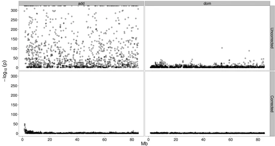
In a first attempt to validate our approach we analyzed cattle chromosome 14 (BTA14) for the traitmilk yield with-out accounting for stratification. This chromosome was cho-sen, becauseDGAT1located in the centromeric region is the underlying gene of a major QTL, which we attempted to detect based on genotype probabilities. The additive effect estimators for the markers in close proximity to DGAT1 showed results correctly reflecting the strong additive effect known to originate from this locus. However, the attempt was hampered by a striking lack of specificity due to stratifi -cation. The results are characterized by extremely lowP-values along the entire chromosome, especially for the additive co-efficients, while the dominance part is less influenced. These results are depicted in the top part of Figure 4. To analyze a possible effect of sample size, we started with 10,000 cows and sequentially increased the number up to 470,000, rep-resenting the entire data set (data not shown). Larger samples did not lead to an improvement; the specificity sub-stantially decreased with an increasing number of cows. When reaching the maximum sample size, false positives were completely covering the association signal. The sub-sequent correction applying a mixed model resulted in an effective adjustment. The bottom part of Figure 4 shows the corrected results for additive and dominance signals, using the complete data set of 470,000 cows with genotype prob-abilities. The direct comparison of the results without and with correction impressively illustrates the effectiveness of the approach. After adjustment, the aforementioned DGAT -QTL can easily be detected at a position of0.5 Mb.
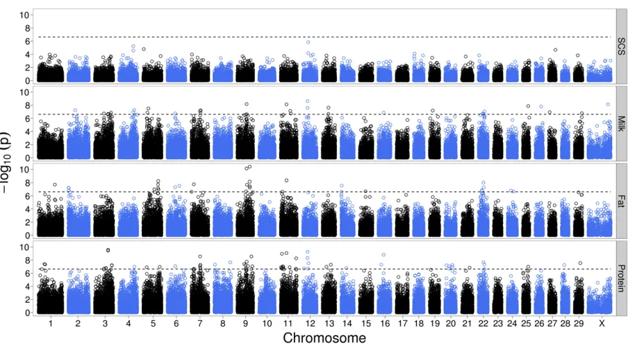
however, dramatically increased the sensitivity for additive signals (data not shown). Therefore, it works as a quick scan for dominance. It might be worth investigating whether this can be improved by the utilization of deeper pedigrees in the calculation of the relationship matrix. Figure 5 is an
illustration of the result of a genome scan for dominance effects. Applying a significance threshold ofP#0.01 after Bonferroni correction, there were no significant results for SCS. For MY, FY, and PY, 29 SNPs on 15 chromosomes, 30 SNPs on 11 chromosomes, and 59 SNPs on 17 chromosomes with significant dominance effects were detected, respec-tively (Table S1). Some chromosomal regions, especially on BTA9 and BTA22, exhibit significant dominance effects for all analyzed yield traits. To further characterize these findings, additional analyses for FY and PY were performed including MY as a covariable in the preadjustment, aiming to reflect the corresponding content traits. Notably, those regions on BTA9 and -22 affecting FY also significantly af-fected fat content, while those affecting PY had no signifi -cant dominance effect for protein content (data not shown). Thus, it can be concluded that the effect in PY is due to an effect on MY, while fat content is directly affected. These two chromosomes seem to harbor QTL for milk yield and fat content displaying considerable dominance effects. QTL for yield traits have been previously described on BTA9 (Wiener et al. 2000) as well as on BTA22 (Ashwell et al. 2004; Harderet al.2006). However, these studies used genotyped sires and daughter-based phenotypes and did thus not iden-tify any dominance effects. Furthermore, significant domi-nance effects were detected on BTA14 within the DGAT1 region. Applying the full model as described below, a domi-nance effect of 0.063 phenotypic standard deviations (sp) along with a significant additive effect of 0.202 sp was found for marker ARS-BFGL-NGS-100480 at 4.36 Mb. This is in general accordance with the divergent effect of the Figure 3 Graphical representation of the specificity to detect dominance
effects as obtained from the multimarker simulation scenario. Compared
are the specificities conditional on family size (daughters per sire) without
any correction for relatedness (black) and after correction applying a linear mixed model (blue).
Figure 4 Analysis of BTA14 for the trait milk yield in a real data set comprising 469,454 cows. They-axis represents the negative decadic logarithm of
theP-values for the additive (left) and dominance (right) effects after Bonferroni correction. Thex-axis gives the position on BTA14 in megabase pairs
according to genome build UMD 3.1. The top panel represents the results without correction. Especially for the additive effects, there is a striking lack of
heterozygous condition compared to the mean of the homo-zygous states found in a study using 1035 Holstein cows genotyped for two DGAT1 polymorphisms (Kuehn et al. 2007).
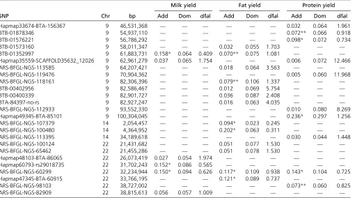
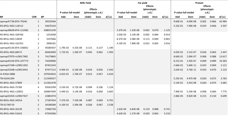
As the dependent variables in this approach are residuals from the previous step, the effect estimators cannot be in-terpreted readily. Thus, an analysis applying the full model is necessary for the markers considered significant to obtain reliable effect estimators. This was conducted for the markers showing significant dominance effects withP#0.01 for MY, FY, and PY. The effect estimators obtained from this model are exemplarily shown for BTA9, -14, and -22 in Table 5 (see alsoTable S1). The markers on BTA9 are distributed across a large chromosomal region ranging from 46.5 to 100.3 Mb. They are characterized by notably high degrees of domi-nance. For milk yield, there is a clear peak around 62 Mb. The highest dominance effect of 0.065sp for this trait was found at marker Hapmap35559-SCAFFOLD35632_12026 at 62.96 Mb. The degree of dominance (d/|a|) = 1.754 and no significant additive effect was detected applying the full model. This is even more pronounced for PY. For this trait, the same marker shows a dominance effect of 0.072spand a d/|a| value of 12.466. Such signals might be missed in studies using breeding values as phenotypes. In this case, however, there are adjacent markers, for which considerable additive effects were detected (Table 5). The same applies for BTA22, where the d/|a| values are generally smaller compared to those for BTA9. In total, there are 10, 12, and 26 SNPs with d/|a| values.2 for MY, FY, and PY, respec-tively (Table S1). For none of these markers was a significant additive effect observed when applying the full model. For
each analyzed yield trait, there is at least one marker showing an additive effect of.0.1spwithP#0.01. These effects would probably have been detectable in studies using daughter-based breeding values, but the considerable dominance effects would be missed. Large-scale studies using breeding values or daugh-ter yield deviations exhibit high statistical power and have suc-cessfully been applied to the identification of numerous QTL in dairy cattle. However, our results emphasize the need to use direct phenotypes to better understand the genetic architecture of traits.
Conclusion
The detection of dominance effects relies on the utilization of direct phenotypes, while classical QTL mapping approaches in dairy cattle employed breeding values of sires based on daughter performance. The implementation of genomic selection schemes in dairy cattle breeding provides a large number of bulls genotyped for dense genome-wide marker panels. Within the current study, these genotypes were used to derive genotype probabilities in female descendants of these bulls. Using these probabilities it is possible to detect significant dominance effects on a genome-wide scale, re-lying on a large sample of phenotyped cows. Together with a two-step mixed model approach to account for relationship among animals, the approach is computationally not chal-lenging and applicable to data sets of .106cows. The ap-plication of this approach could substantially enhance our knowledge about the genetic architecture of performance and functional traits in dairy cattle. The introduced method could also be extended for use in genomic prediction, in-cluding the enlargement of reference populations or the Figure 5 Manhattan plots representing the results of a genome scan for dominance, applying correction for relatedness among animals in a two-step mixed-model approach. Analyzed were the traits somatic cell score (SCS), milk yield, fat yield, and protein yield. Shown are the negative decadic
prediction of individual performance accounting for nonad-ditive genetic effects.
Acknowledgments
This study was financially supported by the German Fed-eral Ministry for Education and Research in the context of the Funktionelle Genomanalyse im Tierischen Organismus (FUGATO+, or Functional Genome Analysis in Animal Organisms) project GenoTrack (grant 0315134A) and the competence networksSynbreed(grant 0315528F) and Phä-nomics(grant 0315536D).
Literature Cited
Ashwell, M. S., D. W. Heyen, T. S. Sonstegard, C. P. Van Tassell, Y.
Da et al., 2004 Detection of quantitative trait loci affecting
milk production, health, and reproductive traits in Holstein cat-tle. J. Dairy Sci. 87: 468–475.
Aulchenko, Y. S., D. J. de Koning, and C. Haley, 2007 Genomewide rapid association using mixed model and regression: a fast and simple method for genomewide pedigree-based quantitative trait loci association analysis. Genetics 177: 577–585.
Elston, R. C., and J. Stewart, 1971 A general model for the ge-netic analysis of pedigree data. Hum. Hered. 21: 523–542. Gilmour, A. R., R. Thompson, and B. R. Cullis, 1995 Average
in-formation REML: an efficient algorithm for variance parameter estimation in linear mixed models. Biometrics 51: 1440–1450.
Guo, S. W., and E. A. Thompson, 1992 A Monte Carlo method for combined segregation and linkage analysis. Am. J. Hum. Genet. 51: 1111–1126.
Grisart, B., W. Coppieters, F. Farnir, L. Karim, C. Ford et al., 2002 Positional candidate cloning of a QTL in dairy cattle: identification of a missense mutation in the bovine DGAT1 gene with major effect on milk yield and composition. Genome Res. 12: 222–231.
Habier, D., J. Tetens, F. R. Seefried, P. Lichtner, and G. Thaller, 2010 The impact of genetic relationship information on geno-mic breeding values in German Holstein cattle. Genet. Sel. Evol. 42: 5.
Haley, C. S., and S. A. Knott, 1992 A simple regression method for mapping quantitative trait loci in line crosses using flanking markers. Heredity 69: 315–324.
Harder, B., J. Bennewitz, N. Reinsch, G. Thaller, H. Thomsenet al., 2006 Mapping of quantitative trait loci for lactation persis-tency traits in German Holstein dairy cattle. J. Anim. Breed. Genet. 123: 89–96.
Hayes, B., and M. E. Goddard, 2001 The distribution of the effects of genes affecting quantitative traits in livestock. Genet. Sel. Evol. 33: 209–229.
Henshall, J. M., and B. Tier, 2003 An algorithm for sampling de-scent graphs in large complex pedigrees efficiently. Genet. Res. 81: 205–212.
Kenward, M. G., and J. H. Roger, 1997 The precision of fixed effects estimates from restricted maximum likelihood. Biomet-rics 53: 983–997.
Khatkar, M. S., P. C. Thomson, I. Tammen, and H. W. Raadsma, 2004 Quantitative trait loci mapping in dairy cattle: review and meta-analysis. Genet. Sel. Evol. 36: 163–190.
Table 5 Results from applying the full mixed model to the real data set for selected markers and chromosomes
Milk yield Fat yield Protein yield
SNP Chr bp Add Dom d/|a| Add Dom d/|a| Add Dom d/|a|
Hapmap33674-BTA-156367 9 46,531,368 — — — — — — 0.032 0.064 1.961
BTB-01878346 9 54,937,110 — — — — — — 0.072** 0.066 0.918
BTB-01576221 9 56,786,292 — — — — — — 0.098* 0.072 0.734
BTB-01573160 9 58,011,347 — — — 0.032 0.055 1.703 — — —
BTB-01352997 9 61,883,731 0.158* 0.064 0.409 0.070** 0.075 1.081 — — —
Hapmap35559-SCAFFOLD35632_12026 9 62,961,279 0.037 0.065 1.754 — — — 0.006 0.072 12.466
ARS-BFGL-NGS-113585 9 64,207,421 — — — 0.018 0.064 3.563 — — —
ARS-BFGL-NGS-119476 9 70,904,362 — — — — — — 0.005 0.060 11.968
ARS-BFGL-NGS-118161 9 82,306,396 — — — 0.079** 0.106 1.337 — — —
BTB-00402956 9 82,586,467 — — — 0.012 0.069 5.754 — — —
BTB-00400339 9 82,901,727 — — — 0.036 0.087 2.408 — — —
BTA-84397-no-rs 9 82,927,247 — — — 0.016 0.063 4.035 — — —
ARS-BFGL-NGS-112933 9 93,552,330 — — — — — — 0.010 0.080 8.269
Hapmap49345-BTA-85101 9 100,304,045 — — — — — — 0.236* 0.297 1.256
ARS-BFGL-NGS-107379 14 2,054,457 — — — 0.094* 0.023 0.245 — — —
ARS-BFGL-NGS-100480 14 4,364,952 — — — 0.202* 0.063 0.311 — — —
ARS-BFGL-NGS-113395 14 34,189,618 — — — — — — 0.030 0.044 1.448
ARS-BFGL-NGS-100124 22 21,431,682 — — — 0.051 0.077 1.530 — — —
ARS-BFGL-NGS-65462 22 21,455,286 — — — 0.051 0.078 1.530 — — —
Hapmap48103-BTA-86065 22 26,073,419 0.027 0.054 1.974 — — — — — —
Hapmap60793-rs29018735 22 31,702,243 0.152* 0.086 0.565 — — — — — —
ARS-BFGL-NGS-60299 22 32,234,944 0.150* 0.094 0.626 0.117* 0.109 0.938 0.143* 0.104 0.725
Hapmap47345-BTA-60915 22 33,766,195 — — — 0.121* 0.089 0.737 — — —
ARS-BFGL-NGS-98103 22 38,727,002 — — — — — — 0.073** 0.060 0.825
ARS-BFGL-NGS-82909 22 38,815,613 0.056 0.057 1.009 — — — — — —
Given are the additive (Add) and dominance (Dom) effects obtained from the full model as well as the degrees of dominance (d/|a|) for SNP markers showing significant (P#
0.01) dominance effects in the two-step genome scan. The markers on BTA9, -14, and -22 are exemplarily summarized (for a full list seeTable S1). Effects are given in phenotypic standard deviations (sP). Chr and bp are the cattle chromosome and the position in base pairs according to genome build UMD 3.1. Significance of additive
Kuehn, C., C. Edel, R. Weikard, and G. Thaller, 2007 Dominance and parent-of-origin effects of coding and non-coding alleles at the acylCoA-diacylglycerol-acyltransferase (DGAT1) gene on milk production traits in German Holstein cows. BMC Genet. 8: 62.
Liu, Z., F. R. Seefried, F. Reinhardt, S. Rensing, G. Thaller et al., 2011 Impacts of both reference population size and inclusion of a residual polygenic effect on the accuracy of genomic pre-diction. Genet. Sel. Evol. 43: 19.
Lund, M. S., A. P. W. de Roos, A. G. de Vries, T. Druet, V. Ducroqc
et al., 2010 Improving genomic prediction by EuroGenomics
collaboration, p. 150 inProceedings of the 9th World Congress on
Genetics Applied Livestock Production, German Society for Animal
Science, Leipzig, Germany.
Purcell, S., B. Neale, K. Todd-Brown, L. Thomas, M. A. Ferreira
et al., 2007 PLINK: a tool set for whole-genome association
and population-based linkage analyses. Am. J. Hum. Genet. 81: 559–575.
R Development Core Team, 2008 R: A Language and Environment
for Statistical Computing. R Foundation for Statistical
Comput-ing, Vienna.
Riquet, J., W. Coppieters, N. Cambisano, J. J. Arranz, P. Berziet al., 1999 Fine-mapping of quantitative trait loci by identity by
descent in outbred populations: application to milk production in dairy cattle. Proc. Natl. Acad. Sci. USA 96: 9252–9257. Spelman, R. J., C. A. Ford, P. McElhinney, G. C. Gregory, and R. G.
Snell, 2002 Characterization of the DGAT1 gene in the New Zealand dairy population. J. Dairy Sci. 85: 3514–3517. Thaller, G., W. Kramer, A. Winter, B. Kaupe, G. Erhardt et al.,
2003 Effects of DGAT1 variants on milk production traits in German cattle breeds. J. Anim. Sci. 81: 1911–1918.
Weller, J. I., M. Golik, E. Seroussi, E. Ezra, and M. Ron, 2003 Population-wide analysis of a QTL affecting milk-fat production in the Israeli Holstein population. J. Dairy Sci. 86: 2219–2227.
Wiener, P., I. Maclean, J. L. Williams, and J. A. Woolliams, 2000 Testing for the presence of previously identified QTL for milk production traits in new populations. Anim. Genet. 31: 385–395.
Winter, A., W. Kramer, F. A. Werner, S. Kollers, S. Kata et al., 2002 Association of a lysine-232/alanine polymorphism in a bovine gene encoding acyl-CoA:diacylglycerol acyltransferase (DGAT1) with variation at a quantitative trait locus for milk fat content. Proc. Natl. Acad. Sci. USA 99: 9300–9305.
GENETICS
Supporting Information
http://www.genetics.org/lookup/suppl/doi:10.1534/genetics.112.144535/-/DC1
Novel Use of Derived Genotype Probabilities
to Discover Signi
fi
cant Dominance Effects
for Milk Production Traits in Dairy Cattle
Teide-Jens Boysen, Claas Heuer, Jens Tetens, Fritz Reinhardt, and Georg Thaller
File S1
R-‐script with the simulation routines as well as the R-‐ and Shell-‐scripts used for data analysis
Available for download at http://www.genetics.org/lookup/suppl/doi:10.1534/genetics.112.144535/-‐/DC1.
File S2
Supporting Data
Available for download at http://www.genetics.org/lookup/suppl/doi:10.1534/genetics.112.144535/-‐/DC1. The archive contains all files to redo the analyisis of the real data set from Boysen,
Heuer, Tetens, Reinhardt and Thaller: A novel approach for dissecting the genetic architecture of performance and functional traits in dairy cattle.
The archive contains the following files:
bulls.bed/bulls.bim/bulls.fam: 50k SNP data of sires and maternal grandsires in a binary plink format. Map data is included in bulls.bim and also available in Bovine_50k.map.
pedinfo.csv: Sire and maternal grandsire for each cow.
cow_phenotypes.csv: Cow's yield deviations for the relevant traits.
The animal identifiers are anonymized and represent a running integer. The true identifiers cannot be retrieved from the data.
Table S1 P-‐values and effects obtained from reanalysis applying the full mixed model for markers with significant dominance effects in the two-‐step genome scan. Given are the SNP-‐name, the cattle chromosome (CHR) and the position in basepairs (BP) along with the p-‐values for the additive (Add) and dominance (Dom) effect and the effects expressed as phenotypic standard deviations as well as the degree of dominance (d/|a|). Additive effects are expressed as absolute values.
Milk Yield Fat yield Protein
P-‐value full model (phenotypic s.d.) Effects P-‐value full model
Effects (phenotypic
s.d.) P-‐value full model
Effects (phenotypic
s.d.)
SNP CHR BP Add Dom |Add| Dom d/|a| Add Dom |Add| Dom d/|a| Add Dom |Add| Dom d/|a|
Hapmap47738-‐BTA-‐79246 1 39259346 9.60E-‐01 4.09E-‐08 0.002 0.066 42.984
ARS-‐BFGL-‐NGS-‐118112 1 43670143 5.22E-‐01 7.00E-‐08 0.019 0.066 3.507
Hapmap38658-‐BTA-‐121982 1 108031239 3.37E-‐02 1.33E-‐08 0.062 0.070 1.125
ARS-‐BFGL-‐NGS-‐104760 2 2254298
2.03E-‐03 2.19E-‐08 0.092 0.084 0.914
ARS-‐BFGL-‐NGS-‐53839 2 3197666
8.37E-‐04 2.08E-‐08 0.113 0.090 0.801
ARS-‐BFGL-‐NGS-‐102353 2 3900181
4.10E-‐01 7.88E-‐08 0.022 0.065 3.016
Hapmap43136-‐BTA-‐106852 2 45085937 1.79E-‐02 4.25E-‐08 0.115 0.137 1.190
ARS-‐BFGL-‐NGS-‐68572 3 60362069 1.71E-‐01 1.36E-‐07 0.045 0.062 1.393 4.03E-‐01 1.51E-‐07 0.026 0.063 2.447
Hapmap57979-‐rs29017982 3 74179845 8.66E-‐01 2.09E-‐07 0.006 0.088 13.617
Hapmap43144-‐BTA-‐107773 3 74204900 8.21E-‐01 1.92E-‐07 0.009 0.089 10.365
Hapmap57348-‐rs29011302 3 87451543 2.66E-‐01 5.60E-‐11 0.033 0.069 2.121
Hapmap53568-‐rs29013441 3 87477115 4.40E-‐01 6.16E-‐08 0.024 0.056 2.343 2.63E-‐01 3.76E-‐11 0.033 0.070 2.123
UA-‐IFASA-‐5880 3 107043933 6.81E-‐01 1.76E-‐07 0.013 0.057 4.424
BTB-‐01641394 3 112340357 5.25E-‐01 4.97E-‐08 0.020 0.073 3.762
ARS-‐BFGL-‐NGS-‐37809 3 112361478 5.14E-‐01 3.91E-‐08 0.020 0.074 3.681
ARS-‐BFGL-‐NGS-‐75789 4 93562599 3.53E-‐02 6.72E-‐08 0.094 0.106 1.124
ARS-‐BFGL-‐NGS-‐110051 4 100847049 5.94E-‐01 3.14E-‐08 0.016 0.060 3.665
7.90E-‐01 5.24E-‐08 0.008 0.060 7.775
Hapmap55454-‐rs29027427 5 22881974 2.86E-‐05 9.82E-‐08 0.215 0.150 0.699
ARS-‐BFGL-‐NGS-‐34254 5 27287454 7.37E-‐03 7.33E-‐08 0.087 0.069 0.791
BTB-‐01740719 5 34180584 4.10E-‐01 2.39E-‐08 0.026 0.067 2.538
ARS-‐BFGL-‐NGS-‐26139 5 72982750 1.62E-‐04 6.83E-‐08 0.119 0.088 0.741
Hapmap47511-‐BTA-‐114200 5 98579869 1.64E-‐01 3.76E-‐08 0.038 0.057 1.517
Hapmap47185-‐BTA-‐114173 5 99044605 5.09E-‐01 4.41E-‐09 0.017 0.069 3.976
ARS-‐BFGL-‐NGS-‐37981 5 100800335 3.49E-‐01 6.90E-‐08 0.024 0.063 2.578
ARS-‐BFGL-‐NGS-‐28067 5 109252813 1.79E-‐01 9.85E-‐08 0.067 0.142 2.112
Hapmap24252-‐BTA-‐147305 6 50627149
7.36E-‐06 4.34E-‐08 0.213 0.162 0.760
BTB-‐01794972 6 51729279 7.25E-‐01 1.11E-‐07 0.020 0.175 8.574
2.36E-‐01 5.24E-‐08 0.066 0.183 2.764
BTB-‐00264565 6 79705920
3.28E-‐02 2.12E-‐08 0.131 0.213 1.625
ARS-‐BFGL-‐NGS-‐114934 7 15921536 7.69E-‐01 8.37E-‐09 0.009 0.080 9.240
Hapmap47101-‐BTA-‐78263 7 16564424 8.77E-‐01 8.00E-‐08 0.006 0.103 17.032
ARS-‐BFGL-‐NGS-‐3043 7 17528449 3.47E-‐01 2.28E-‐07 0.039 0.118 2.982
BTB-‐01641665 7 57575330 7.41E-‐06 8.28E-‐08 0.139 0.066 0.472 2.56E-‐07 3.37E-‐09 0.152 0.074 0.488
Hapmap59042-‐rs29025710 7 57703177 1.99E-‐11 5.65E-‐08 0.195 0.066 0.337
ARS-‐BFGL-‐NGS-‐33130 7 58667344 4.71E-‐01 6.00E-‐08 0.025 0.082 3.252
ARS-‐BFGL-‐NGS-‐10904 7 59829599 6.80E-‐06 3.56E-‐08 0.152 0.088 0.581
ARS-‐BFGL-‐NGS-‐108586 7 59862113 2.09E-‐05 1.36E-‐07 0.135 0.078 0.575
ARS-‐BFGL-‐NGS-‐29389 7 60585197 2.25E-‐03 8.98E-‐08 0.094 0.059 0.631
BTB-‐00315489 7 62266710 2.80E-‐06 4.54E-‐08 0.153 0.075 0.490
BTB-‐01956236 8 4372100
6.41E-‐05 4.45E-‐08 0.173 0.111 0.644
ARS-‐BFGL-‐NGS-‐39754 8 106264025
2.08E-‐03 9.19E-‐09 0.091 0.061 0.676
Hapmap33674-‐BTA-‐156367 9 46531368 3.17E-‐01 3.91E-‐08 0.032 0.064 1.961
BTB-‐01878346 9 54937110 1.37E-‐02 3.19E-‐08 0.072 0.066 0.918
BTB-‐01576221 9 56786292 6.79E-‐04 1.52E-‐07 0.098 0.072 0.734
BTB-‐01573160 9 58011347 2.23E-‐01 1.27E-‐07 0.032 0.055 1.703
BTB-‐01352997 9 61883731 7.63E-‐06 4.17E-‐09 0.158 0.064 0.409 2.12E-‐02 5.02E-‐11 0.070 0.075 1.081
Hapmap35559-‐
SCAFFOLD35632_12026 9 62961279 2.85E-‐01 1.35E-‐07 0.037 0.065 1.754 8.61E-‐01 9.78E-‐09 0.006 0.072 12.466
ARS-‐BFGL-‐NGS-‐113585 9 64207421 4.94E-‐01 1.17E-‐08 0.018 0.064 3.563
ARS-‐BFGL-‐NGS-‐119476 9 70904362 8.69E-‐01 6.14E-‐08 0.005 0.060 11.968
ARS-‐BFGL-‐NGS-‐118161 9 82306396 1.84E-‐02 5.27E-‐09 0.079 0.106 1.337
BTB-‐00400339 9 82901727 2.01E-‐01 2.07E-‐11 0.036 0.087 2.408
BTA-‐84397-‐no-‐rs 9 82927247 5.54E-‐01 2.74E-‐08 0.016 0.063 4.035
ARS-‐BFGL-‐NGS-‐112933 9 93552330 7.65E-‐01 3.18E-‐09 0.010 0.080 8.269
Hapmap49345-‐BTA-‐85101 9 100304045 3.56E-‐03 5.34E-‐08 0.236 0.297 1.256
BTB-‐00448829 11 2140304
5.67E-‐01 1.13E-‐07 0.027 0.110 4.144
ARS-‐BFGL-‐NGS-‐64657 11 5872611
4.85E-‐02 1.79E-‐07 0.083 0.092 1.118
ARS-‐BFGL-‐NGS-‐35216 11 7585747
5.10E-‐03 3.82E-‐10 0.082 0.064 0.780
ARS-‐BFGL-‐NGS-‐110311 11 8185823
7.43E-‐02 2.10E-‐07 0.084 0.122 1.462
BTB-‐01569510 11 9755667
3.03E-‐01 2.17E-‐07 0.034 0.091 2.704
ARS-‐BFGL-‐NGS-‐2493 11 13114243
1.53E-‐03 9.30E-‐08 0.104 0.079 0.767
BTB-‐00463178 11 16345034
1.98E-‐06 1.51E-‐07 0.149 0.058 0.387
BTB-‐00463351 11 16374116
1.31E-‐06 8.30E-‐08 0.151 0.058 0.387
ARS-‐BFGL-‐NGS-‐117280 11 37783495 1.85E-‐01 4.55E-‐09 0.041 0.068 1.653 4.48E-‐02 2.81E-‐09 0.054 0.072 1.347 7.27E-‐02 5.61E-‐10 0.053 0.074 1.390
BTB-‐01180855 11 58684365
1.70E-‐03 8.81E-‐08 0.112 0.079 0.706
ARS-‐BFGL-‐NGS-‐1065 11 62868207 4.25E-‐06 1.02E-‐07 0.141 0.066 0.467
BTA-‐101061-‐no-‐rs 11 66450428 1.66E-‐03 1.22E-‐07 0.124 0.082 0.660
ARS-‐BFGL-‐NGS-‐116589 11 100901534
5.90E-‐01 1.34E-‐07 0.016 0.053 3.286
ARS-‐BFGL-‐NGS-‐37815 11 101829398
4.70E-‐04 3.85E-‐09 0.139 0.124 0.892
ARS-‐BFGL-‐BAC-‐775 12 6987206 7.57E-‐01 1.23E-‐07 0.009 0.057 6.207
ARS-‐BFGL-‐NGS-‐116664 12 30609095 2.52E-‐02 1.55E-‐09 0.096 0.103 1.072 1.90E-‐02 3.88E-‐10 0.096 0.109 1.136
ARS-‐BFGL-‐BAC-‐15026 12 30668435 4.38E-‐01 1.40E-‐08 0.036 0.122 3.385 2.96E-‐01 2.63E-‐09 0.046 0.130 2.810
ARS-‐BFGL-‐NGS-‐88871 12 33535830 8.70E-‐01 1.28E-‐07 0.006 0.080 13.093
ARS-‐BFGL-‐NGS-‐100956 12 37110042 1.79E-‐02 1.79E-‐08 0.167 0.245 1.471
BTA-‐31928-‐no-‐rs 13 25842073
2.09E-‐02 9.93E-‐08 0.127 0.142 1.120
ARS-‐BFGL-‐NGS-‐118784 13 38656618 7.54E-‐01 1.35E-‐07 0.010 0.056 5.669
ARS-‐BFGL-‐NGS-‐102990 13 38943133 4.01E-‐01 7.45E-‐09 0.028 0.063 2.259
ARS-‐BFGL-‐NGS-‐76148 13 54829615
1.25E-‐02 3.51E-‐08 0.138 0.154 1.116
ARS-‐BFGL-‐NGS-‐107379 14 2054457 3.21E-‐04 5.39E-‐02 0.094 0.023 0.245
ARS-‐BFGL-‐NGS-‐100480 14 4364952 4.98E-‐13 2.96E-‐06 0.202 0.063 0.311
ARS-‐BFGL-‐NGS-‐115927 15 39469268
1.73E-‐02 1.92E-‐07 0.086 0.104 1.205
ARS-‐BFGL-‐NGS-‐33988 16 19828569 7.56E-‐01 2.81E-‐08 0.009 0.060 6.370
Hapmap42533-‐BTA-‐38667 16 34938163 5.89E-‐05 1.78E-‐09 0.146 0.101 0.692
Hapmap45766-‐BTA-‐38696 16 35896376 2.42E-‐02 1.52E-‐07 0.089 0.086 0.970
ARS-‐BFGL-‐NGS-‐63687 19 20635700 4.94E-‐01 4.59E-‐08 0.027 0.087 3.184
ARS-‐BFGL-‐NGS-‐70354 20 9028131 1.11E-‐02 3.36E-‐08 0.118 0.145 1.234
ARS-‐BFGL-‐NGS-‐12319 20 26330033 1.49E-‐02 1.44E-‐07 0.186 0.288 1.548
ARS-‐BFGL-‐NGS-‐58033 20 26397183 1.22E-‐02 6.34E-‐08 0.191 0.293 1.531
Hapmap42701-‐BTA-‐84483 20 47935136 3.68E-‐06 3.72E-‐08 0.181 0.105 0.578
BTB-‐01164745 20 48003042 5.20E-‐06 7.50E-‐08 0.177 0.102 0.574
ARS-‐BFGL-‐NGS-‐110784 21 51031411
5.08E-‐01 1.08E-‐07 0.019 0.062 3.199
ARS-‐BFGL-‐NGS-‐100124 22 21431682 1.21E-‐01 1.24E-‐07 0.051 0.077 1.530
ARS-‐BFGL-‐NGS-‐65462 22 21455286 1.16E-‐01 9.30E-‐08 0.051 0.078 1.530
Hapmap48103-‐BTA-‐86065 22 26073419 3.82E-‐01 2.39E-‐07 0.027 0.054 1.974
Hapmap60793-‐rs29018735 22 31702243 3.88E-‐04 1.34E-‐07 0.152 0.086 0.565
ARS-‐BFGL-‐NGS-‐60299 22 32234944 1.06E-‐03 1.63E-‐07 0.150 0.094 0.626 3.44E-‐03 5.42E-‐09 0.117 0.109 0.938 1.03E-‐03 1.30E-‐08 0.143 0.104 0.725
Hapmap47345-‐BTA-‐60915 22 33766195 1.70E-‐04 3.64E-‐08 0.121 0.089 0.737
ARS-‐BFGL-‐NGS-‐98103 22 38727002 1.76E-‐02 2.33E-‐08 0.073 0.060 0.825
ARS-‐BFGL-‐NGS-‐82909 22 38815613 7.00E-‐02 7.79E-‐08 0.056 0.057 1.009
ARS-‐BFGL-‐NGS-‐102332 24 21918990
9.47E-‐01 4.91E-‐08 0.002 0.087 40.994
ARS-‐BFGL-‐NGS-‐40316 24 39414051
4.09E-‐01 1.54E-‐07 0.022 0.065 2.958
ARS-‐BFGL-‐NGS-‐13985 25 35071379 3.40E-‐01 1.12E-‐08 0.036 0.085 2.344 6.09E-‐01 8.78E-‐08 0.018 0.081 4.402
ARS-‐BFGL-‐NGS-‐39928 26 38846841 2.16E-‐04 1.21E-‐08 0.152 0.092 0.602