Inference Under a Wright-Fisher Model Using an Accurate Beta Approximation

GENETICS | INVESTIGATION

Inference Under a Wright-Fisher Model Using an

Accurate Beta Approximation

Paula Tataru,1_{Thomas Bataillon, and Asger Hobolth}

Bioinformatics Research Centre, Aarhus University, Aarhus C 8000, Denmark

ABSTRACTThe large amount and high quality of genomic data available today enable, in principle, accurate inference of evolutionary histories of observed populations. The Wright-Fisher model is one of the most widely used models for this purpose. It describes the stochastic behavior in time of allele frequencies and the influence of evolutionary pressures, such as mutation and selection. Despite its simple mathematical formulation, exact results for the distribution of allele frequency (DAF) as a function of time are not available in closed analytical form. Existing approximations build on the computationally intensive diffusion limit or rely on matching moments of the DAF. One of the moment-based approximations relies on the beta distribution, which can accurately describe the DAF when the allele frequency is not close to the boundaries (0 and 1). Nonetheless, under a Wright-Fisher model, the probability of being on the boundary can be positive, corresponding to the allele being either lost orfixed. Here we introduce the beta with spikes, an extension of the beta approximation that explicitly models the loss andfixation probabilities as two spikes at the boundaries. We show that the addition of spikes greatly improves the quality of the approximation. We additionally illustrate, using both simulated and real data, how the beta with spikes can be used for inference of divergence times between populations with comparable performance to an existing state-of-the-art method.

KEYWORDSWright-Fisher; beta; pure genetic drift; linear evolutionary pressures; divergence times

A

DVANCES in sequencing technologies have revolution-ized the collection of genomic data, increasing both the volume and quality of available sequenced individuals from a large variety of populations and species (Romiguier et al.

2014; Gudbjartsson et al. 2015). These data, which may involve up to millions of single-nucleotide polymorphisms (SNPs), contain information about the evolutionary history of the observed populations. There has been a great focus in the recent years on inferring such histories, and to this end, one of the most widely used models is the Wright-Fisher model (Gautier et al. 2010; Sirén et al. 2011; Malaspinas

et al.2012; Pickrell and Pritchard 2012; Gautier and Vitalis 2013; Steinrückenet al.2014; Terhorstet al.2015).

The Wright-Fisher model characterizes the evolution of a randomly mating population of finite size in discrete nonoverlapping generations. The model describes the

sto-chastic behavior in time of the number of copies (frequency) of alleles at a locus. The frequency is influenced by a series of factors, such as random genetic drift, mutations, migrations, selection, and changes in population size. When inferring the evolutionary history of a population, the effects of the different factors have to be untangled. Mutation, migration, and selection affect the allele frequency in a deterministic manner (Ewens 2004). We collectively refer to these as

evolutionary pressures. The frequency also varies from one generation to the next as a result of random sampling of afinite-sized population (random genetic drift). Mutations and migrations result in linear changes of the sampling probability, while selection is a nonlinear pressure (Kimura 1964; Crow and Kimura 1970) and therefore is more diffi-cult to study analytically.

A crucial step for carrying out statistical inference in the Wright-Fisher model is determination of thedistribution of allele frequency(DAF) as a function of time, conditional on an initial frequency. Even though the Wright-Fisher model has a very simple mathematical formulation, no tractable analytical form exists for the DAF (Ewens 2004). Therefore, various approximations have been developed, ranging from purely analytical to purely numerical. They generally either

Copyright © 2015 by the Genetics Society of America doi: 10.1534/genetics.115.179606

Manuscript received June 19, 2015; accepted for publication August 22, 2015; published Early Online August 26, 2015.

Supporting information is available online at www.genetics.org/lookup/suppl/ doi:10.1534/genetics.115.179606/-/DC1

1_{Corresponding author: Bioinformatics Research Centre, Aarhus University, C. F.} Møllers Allé 8, Aarhus C 8000, Denmark. E-mail: [email protected]

build on the diffusion limit of the Wright-Fisher model or rely on matching moments of the true DAF. Both types of approximations have been used successfully for inference of populations divergence times (Sirénet al.2011; Gautier and Vitalis 2013), populations admixture (Pickrell and Pritchard 2012), SNPs under selection (Gautier et al.

2010), and selection coefficients from time-serial data (Malaspinaset al.2012; Steinrückenet al.2014; Terhorst

et al.2015).

Wright (1945) was thefirst to use the diffusion approx-imation to determine the stationary DAF. Kimura (1955) solved the diffusion limit and found the time-dependent distribution for pure genetic drift, and Crow and Kimura (1956) extended the solution to include linear evolutionary pressures. However, these approaches contain infinite sums, making their use cumbersome in practice. After decades dominated by inference based on the dual coalescent pro-cess (Rosenberg and Nordborg 2002; Hobanet al. 2012), diffusion has recently received increasing attention, and researchers have started to investigate other ways to solve analytically or approximate the diffusion equation (McKane and Waxman 2007; Waxman 2011; Malaspinaset al.2012; Song and Steinrücken 2012; Zhaoet al.2013; Steinrücken

et al.2013, 2014).

Moment-based approximations are less ambitious in that they aim atfitting mathematically convenient distributions by equating thefirst moments of the true DAF. Such approxima-tions typically use either the normal distribution (Nicholson

et al.2002; Coopet al.2010; Gautieret al.2010; Pickrell and Pritchard 2012; Terhorstet al.2015) or the beta distribution (Balding and Nichols 1995, 1997; Sirén et al. 2011; Sirén 2012). The rationale behind the use of these distributions is twofold. First, they are motivated by the diffusion limit: the normal distribution is the resulting DAF when drift is small (Nicholsonet al.2002), while the beta distribution is the stationary DAF under linear evolutionary pressures (Wright 1945; Crow and Kimura 1956). Second, they are entirely determined by their mean and variance. One major difference between the two is their support. Because the nor-mal distribution is defined over the whole real line, it needs to be truncated to [0,1] (Nicholsonet al. 2002; Coopet al.

2010; Gautieret al.2010). The truncated normal distribution has two atoms at 0 and 1 (corresponding to the allele being lost orfixed) containing the densities in the intervalsð2N;0 and½1;NÞ, respectively. However, the truncation procedure leads to a variance that no longer matches the variance of the true DAF (Gautier and Vitalis 2013). Alternatively, the full distribution can be applied for intermediary frequencies only, when the probabilities of lying outside the 0 and 1 boundaries are small and therefore can be ignored (Pickrell and Pritchard 2012; Terhorstet al.2015). Unlike the normal distribution, the beta distribution has the interval ½0;1as support, but because of its continuous nature, the probabil-ities at the boundaries will always be 0. Under a Wright-Fisher model, the loss and fixation events have a positive probability. The beta distribution provides a goodfit for

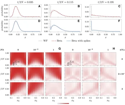
in-termediary frequencies but fails at capturing the nonzero boundary probabilities, as illustrated for pure genetic drift in Figure 1, A–C. When time is small, most of the probability mass is found close to the initial value x0 (Figure 1A). As time becomes larger, the allele frequency drifts away fromx0, and more and more probability accumulates at the boundaries (Figure 1, B and C).

Here we propose an accurate extension of the beta dis-tribution under linear evolutionary pressures called beta with spikes that explicitly models the probabilities at the boundaries. We show that the addition of spikes greatly improves thefit to the true DAF. We use simulation experi-ments and published chimpanzee exome data to demon-strate that beta with spikes can be used for inference of population divergence times under pure genetic drift with performance comparable to that of a state-of-the-art diffu-sion-based method (Gautier and Vitalis 2013) and less com-putational burden. We additionally discuss how beta with spikes can be used in future development to account for variable population size and selection.

Beta with Spikes Approximation

Consider a diploid randomly mating population of size 2N

and a biallelic locus with alleles A1 and A2. Under a Wright-Fisher model, the count of one of the alleles,

A1, at the discrete generation t is a random variable

Zt2 f0;1;. . .;2Ng. LetXt¼Zt=ð2NÞbe the corresponding

allele frequency. The evolution ofZt is shaped by random

genetic drift and evolutionary pressures that affect the sam-pling probability (Ewens 2004). We capture the joint effect of the evolutionary pressures in gðxÞ, a polynomial in the allele frequency 0#x#1. Conditional on Zt,Ztþ1 follows

a binomial distribution (Ewens 2004)

Ztþ1jZt¼zt Bin

2N; gðxtÞ

(1)

Here we consider only linear evolutionary pressures, such as mutation and migration. ThengðxÞtakes the form

gðxÞ ¼ ð12aÞxþb (2)

BecausegðxÞrepresents the sampling probability in equation (1), we must have 0#gðxÞ#1, for all 0#x#1. From this we find that a andb satisfy 0#b#a#1. The case where

a¼1, for whichgðxÞ ¼b, for all 0#x#1, has no biological meaning, and we therefore assume thata6¼1.

Under pure genetic drift,a¼b¼0. If mutations happen with probabilitiesu(fromA1 toA2) andv(fromA2 to A1), thena¼uþvandb¼v. Migration can be modeled, for ex-ample, by assuming that individuals can migrate away from the population under study and that there is an influx of individuals from a large population with constant frequency

xc. Then, with probabilitiesm1 andm2, individuals migrate

from and to the population under study, respectively. We havea¼m1andb¼m2xc. Mutation and migration can be

modeled jointly, resulting ina¼m1þ ð12m1ÞðuþvÞ and

b¼ ð12m1Þvþm2xc. In the following, we treat the general

linear case.

We are interested in the DAFXtconditional onX0¼x0as

a function of the generationt

fðx;tÞ ¼ℙðXt¼xjX0¼x0Þ (3)

For simpler notation, we leave out the explicit condition on

X0 ¼x0and implicit condition on population size and evolu-tionary pressures.

Under the beta approximation, the DAF is (Balding and Nichols 1995)

fBðx;tÞ ¼x

at21ð₁2xÞbt21

Bðat;btÞ

(4)

where Bða;bÞis the beta function. The two shape parameters of the beta distribution are entirely determined by its mean and variance

at ¼ E

½Xt

12E½Xt

VarðXtÞ 21

E½Xt

bt ¼

E½Xt

12E½Xt

VarðXtÞ 2

1

12E½Xt

(5)

Therefore, in order tofitfBtof, we need to calculateE½Xtand

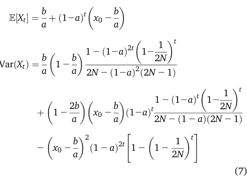
VarðXtÞ. These can be obtained in closed analytical form (see Supporting Information,File S1for a full derivation). The mean is entirely determined by the initial frequency x0 and the parametersaandbof the linear evolutionary pressures, while the variance also depends on the population size. Under pure genetic drift (a¼b¼0), we have

   E½Xt ¼x0

VarðXtÞ ¼x0ð12x0Þ 12

12 1 2N

t

" #

(6) Figure 1 Fit of the beta and beta with spikes approximations for a population of size 2N¼200. (A–F) The true discrete DAF as given by the Wright-Fisher model under pure genetic drift and the corresponding discretized beta (A–C) and beta with spikes (D–F) approximations. The distributions are conditional on an initial frequency x0¼0:2 and for different time points t=2N¼0:035 (A, D), t=2N¼0:115 (B, E), and

t=2N¼0:195 (C, F), wheretis the number of discrete generations that the population has evolved. (G, H) The Hellinger distance between the true DAF and the beta (G) and beta with spikes (H) as a function ofx0andt=2N. Each row and column corresponds to specific values of the scaled

parameters 4Naand 4Nb. The distances corresponding to the distributions from A–F are marked with arrows. The discretization procedure and Hellinger distance are detailed inFile S1.

Whena6¼0, we get

E½Xt ¼

b

aþ ð12aÞ

t

x02

b a

VarðXtÞ ¼

b a

12b

a

12ð12aÞ2t

121 2N

t

2N2ð12aÞ2ð2N21Þ

þ

122b

a x02 b a ð12aÞ

t

12ð12aÞt

121 2N

t

2N2ð12aÞð2N21Þ

2

x02

b a

2

ð12aÞ2t

"

12

12 1 2N

t#

(7)

In the limit of infinite population size, the preceding formulas are equivalent to the mean and variance obtained by Sirén (2012). We note that this equation corrects some typographic errors in Sirén (2012), as confirmed by correspondence with the author (see alsoFile S1).

To account for loss andfixation probabilities, we surround the beta distribution with two spikes

f_B⋆ðx;tÞ ¼ℙðXt¼0Þ dðxÞ þℙðXt¼1Þ dð12xÞ

þℙXt;f0;1g

xa

⋆

t21ð12xÞb ⋆ t21

Ba⋆t;b⋆t

(8)

wheredðxÞis the Dirac delta function, andℙðXt;f0;1gÞ ¼

12ℙðXt¼0Þ2ℙðXt¼1Þ. The incorporation of the loss

andfixation probabilities into the DAF by means of Dirac delta functions has also been used to obtain a complete solution of the diffusion equation (McKane and Waxman 2007).

TofitfB⋆tof, we need to determine the mean and variance of Xtconditional on polymorphism (Xt;f0;1g) and the

probabil-itiesℙðXt¼0ÞandℙðXt¼1Þof loss andfixation, respectively.

GivenE½Xt, VarðXtÞ,ℙðXt¼0Þ, andℙðXt¼1Þ, the conditional

mean and variance can easily be calculated (seeFile S1). The shape parametersa⋆t andb⋆t are calculated as in equation (5),

where the mean and variance are replaced by the conditional mean and variance, respectively. Therefore, we only require a means of calculating the loss and fixation probabilities to fully specify the beta with spikes approximation. We use a recursive approach in which we calculate the proba-bilities forXtþ1by relying on the approximatedfB⋆ðx;tÞ. We

additionally assume that a andb are small to obtain the following approximation for loss andfixation probabilities (seeFile S1for a full derivation):

ℙðXtþ1¼0Þ ℙðXt¼0Þ ð12bÞ2NþℙðXt¼1Þða2bÞ2N

þℙXt;f0;1g

ð12aÞ2N B

a⋆t;b⋆t þ2N

Ba⋆t;b⋆t

ℙðXtþ1¼1Þ ℙðXt¼0Þ b2NþℙðXt¼1Þ ð12aþbÞ2N

þ ℙXt;f0;1g

ð12aÞ2NB

a⋆t þ2N;b⋆t

Ba⋆t;b⋆t

(9)

Figure 1, D–F depicts the beta with spikes approximation for the same cases as in Figure 1, A–C. When time is small (Fig-ure 1, A and D), the beta and beta with spikes distributions are equivalent, but as the time becomes larger, the advantage of adding the spikes becomes evident.

To investigate the approximation quality of the beta with spikes, we calculated the Hellinger distance between the true DAF and the beta and beta with spikes for a range of initial frequenciesx0, timestand parametersaandb(see

File S1 for details). The Hellinger distance lies between 0 and 1, with 0 indicating a perfect match between the two distributions. Figure 1, G and H, shows that the addi-tion of spikes drastically improves the fit of the beta ap-proximation to the true DAF under a Wright-Fisher model. It is apparent from the figure that the beta distribution approximates well the true DAF when it is not close to the boundaries: either the initial frequency is close to 0.5 and the time is not too large or the parametersa orbare large enough to keep the allele frequency away from 0 and 1. The beta with spikes has a more consistent behavior because the corresponding Hellinger distance does not vary as much across the different parameters as it does for the beta distribution.

Inference of Divergence Times

To further illustrate the advantage of incorporating the spikes, we inferred divergence times between populations using both simulated data and exome sequencing data from three chim-panzee subspecies (Bataillonet al.2015).

Populations are represented as successive descendants of a single ancestral population. We assume that after each split, the new populations evolve in isolation (no migration) under pure genetic drift. A rooted tree (Figure 2) can be used to de-scribe the joint history of several present populations, located at the leaves, while the common ancestral population is repre-sented as the root. The dataD ¼ fðzij;nijÞj1#i#I;1#j#Jg

consist ofIindependent SNPs forJpopulations in the present: the (arbitrarily defined) reference (A1) allele countzijin a

sam-ple of sizenij(0#zij#nij) for each locus 1#i#Iand

popula-tion 1#j#J.

Conditional on the topology (i.e., tree without branch lengths), we inferred the scaled branch lengths by numeri-cally maximizing the likelihood of the data.

Likelihood of the data

Assuming Hardy-Weinberg equilibrium, the probability of observingzijalleles in a sample of sizenijgiven the

pop-ulation allele frequency xij is given by the binomial

distribution

ℙzijjnij;xij

¼

n zij x

zij

ij

12xij

nij2zij

(10)

However, the allele frequenciesxij are unobserved, and the

likelihood of the dataDifor SNPiis obtained by integrating

over the unknown allele frequencies

LðDi;Q;pÞ ¼

Z1

0

. . . Z1

0

fðXi1;Xi2;. . .;XiJjQ;pÞ

Y

J j¼1

ℙzijjnij;Xij

dXi1⋯dXiJ (11)

where fðXi1;Xi2;. . .;XiJjQ;pÞ is the joint distribution of

the Xijvalues at the leaves. The likelihood is a function of

the scaled branch lengths, denoted here as Q, and p, the unknown DAF at the root. The joint distribution

fðXi1;Xi2;. . .;XiJjQ;pÞis, in turn, an integral over the allele

frequencies in the ancestral populations, represented as inter-nal nodes in the tree. We approximate the integrals with sums by discretizing the allele frequencies. The discretized joint distribution is then obtained using a peeling algorithm (Felsenstein 1981), where the transition probabilities on each branch are given by the DAF as a function of the branch length (seeFile S1for details). Because the SNPs are assumed to be independent, the full likelihood is a product over the SNPs

LðD;Q;pÞ ¼Y

I i¼1

LðDi;Q;pÞ (12)

Because SNP data contain only polymorphic sites, we further condition the preceding likelihood on polymorphic data as follows:

LðDi;Q;pjpolymorphismiÞ ¼

LðDi;Q;pÞ

ℙðpolymorphismijQ;pÞ

(13)

where

ℙðpolymorphismijQ;pÞ ¼12L

D0

i;Q;p

2LD1_i;Q;p

(14)

HereD0

i andD1i are data corresponding to siteiwhere the

allele was lost orfixed, respectively, in the samples from all populations

D0 i ¼

ð0;nijÞj1#j#J

;D1 i ¼

ðnij;nijÞj1#j#J

(15)

We treatp, the root DAF, as a nuisance distribution, which we assume to be a beta distribution. For a given topology (i.e., tree without branch lengths), the most likely branch lengths and shape parameters of p are recovered by numerically maximizing the likelihood conditional on polymorphism.

Simulated data

Using the topology depicted in Figure 2, we simulated mul-tiple data sets containing independent SNPs under a Wright-Fisher model, given an ancenstral frequency Xi5 sampled

fromp, the root DAF, which we set to be a beta distribution. We used two different scenarios, labeled I and II, summarized in Table 1. Scenario I has a uniformpand large sample sizes, while scenario II is built to produce data that resemble the chimpanzee exome data analyzed later. For this, we used the chimpanzee sample sizes and scaled branch lengths and root DAF as inferred by the beta with spikes on the chimpanzee data (Table 2).

For each simulated data set, we estimated the branch lengths using both the beta and beta with spikes, as described previously. We additionally ran Kim Tree (Gautier and Vitalis 2013) using the default settings. Kim Tree is a method designed for inference of divergence times between popula-tions evolving under pure genetic drift. It uses Kimura’s so-lution to the diffusion limit for the DAF (Kimura 1955) and relies on a Bayesian Markov chain Monte Carlo (MCMC) approach. Here we use the posterior means of the branch lengths reported by this method as point estimates.

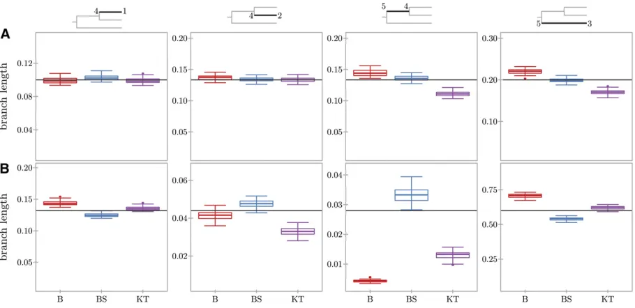
All methods estimated the branches leading to populations 1 and 2 well (Figure 3). Beta with spikes estimates the branch lengths more accurately and with lower variance than the beta approximation (Figure S1). Despite the fact that the spikes’ probabilities do not perfectly match the true loss andfixation probabilities (Figure 1, E and F), this seems to have little effect on the accuracy of branch-length estimation for beta with spikes. For both scenarios, the branch leading to Figure 2 History of three populations in the present. Ancestral population 5 splits in populations 3 and 4, which further splits in populations 2 and 1. For each SNPiand present population

j2 f1;2;3g, the data consist of the sample size nij and allele count zij. The branch length between popula-tions k and j is given as ðt=2NÞ_k/j

and represents the scaled number of generations that population jevolved since the split from the ancestral pop-ulationk. The unknown allele frequen-cies of each population are denoted as

Xij, with 1#j#5.

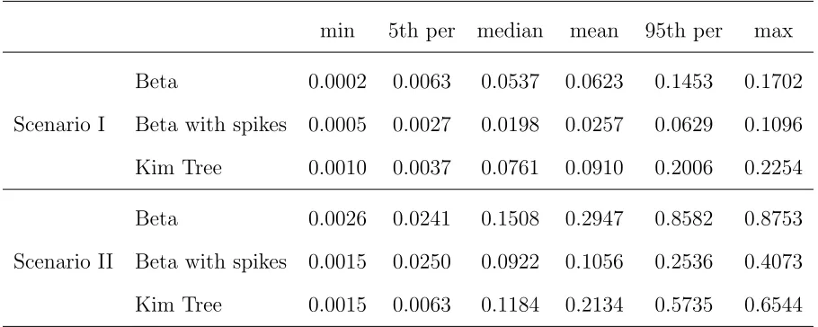
population 2 and the inner branch from the root to popula-tion 4 have similar lengths, but the beta approximapopula-tion and Kim Tree provide a worse estimate for the inner branch. This could be due to the fact that there are no data available resulting directly from the evolution on that branch, making the estimation problem harder. A similar result was obtained by Gautier and Vitalis (2013), who used trees with the same topology. Interestingly, beta with spikes recovers the inner branch much more accurately than either beta or Kim Tree. When measuring the accuracy of the inferred lengths as an average over all four branches (Table S1), it is clear that beta with spikes outperforms Kim Tree for both scenarios.

Chimpanzee data

The chimpanzee data analyzed here consisted of allele counts of autosomal synonymous SNPs obtained from exome se-quencing of the Eastern, Central, and Western chimpanzee subspecies (Bataillonet al.2015) for 11, 12, and 6 individu-als, respectively. From the original data set containing 59,905 synonymous SNPs, wefiltered the SNPs in which there were missing data, obtaining a total of 42,063 SNPs. We inferred the scaled branch lengths (Figure 4 and Table 2) using beta, beta with spikes, and Kim Tree on the full data set and on 50 smaller data sets containing only 10,000 randomly sampled SNPs. Beta with spikes and Kim Tree infer comparable branch lengths, with the exception of the branch leading to the West-ern chimpanzee subspecies. We additionally report in Table 2 the likelihood of the full data calculated using beta with spikes for the branch lengths inferred using the three meth-ods and the ones reported in the original study (Bataillon

et al. 2015). Bataillon et al. (2015) used an approximate Bayesian computation (ABC) approach tofit a demographic model to the synonymous SNPs. Their results are consistent with the results obtained here for the branches leading to the Eastern and Central chimpanzees. However, we obtained very different estimates for the remaining two branches. The likelihoods in Table 2 show that the branch lengths obtained by beta with spikes have the highest likelihood. This does not indicate which of the estimates is most correct be-cause the methods use different modeling approaches. How-ever, it does show that the differences between beta with spikes and beta/Kim Tree/ABC are a direct result of the mod-eling approach and not merely an artifact of the likelihood

numerical optimization being trapped in a local optimum. The discrepancy between the results of beta with spikes and those of ABC is, perhaps, not surprising because the dif-ference in inferred branch lengths seems to correlate with the goodness of fit of the ABC demographic model to the ob-served data. Bataillon et al. (2015) reported that their inferred demographic model shows a very good fit for the Central chimpanzees (absolute and relative difference in inferred branch length 0.017 and 0.386, respectively), a slightly less goodfit for the Eastern chimpanzees (absolute and relative difference in inferred branch length 0.051 and 0.386, respectively), and a poorerfit for the Western chim-panzees (absolute and relative difference in inferred branch length 1.319 and 2.217, respectively).

Data availability

The beta, beta with spikes approximations, inference of di-vergence times, and simulation under a Wright-Fisher model were implemented in Python 2.7. The code is freely available athttps://github.com/paula-tataru/SpikeyTree.

Discussion

We have developed a new approximation to the DAF as a function of time, conditional on an initial frequency, under a Wright-Fisher model with linear evolutionary pressures. Our work provides an accurate extension of the beta approxima-tion (Balding and Nichols 1995, 1997; Sirénet al.2011; Sirén 2012). As noted by Gautier and Vitalis (2013), the beta dis-tribution ignores the possibility of loss orfixation of alleles. We addressed this issue by explicitly modeling the loss and fixation probabilities as two spikes at the boundaries. We showed that the addition of the spikes improves the quality of the approximation and results in more accurate inference of divergence times between populations that have been evolving under pure genetic drift. The DAF obtained as a so-lution of the diffusion equation is exactly the DAF expected under the Wright-Fisher model when the population size is large and the evolutionary pressures are not too strong, while the beta distribution is motivated only by the stationary DAF under linear evolutionary pressures. We therefore expected the beta with spikes to provide a less accurate approximation to the true DAF than the diffusion limit. Nevertheless, we Table 1 Simulation study scenarios

Scenario I Scenario II

ðt=2NÞ4/1 40=ð2200Þ ¼0:1 132=ð2500Þ ¼0:132 ðt=2NÞ4/2 40=ð2150Þ ¼0:133 44=ð2500Þ ¼0:044 ðt=2NÞ5/4 40=ð2150Þ ¼0:133 14=ð2250Þ ¼0:028 ðt=2NÞ5/3 80=ð2200Þ ¼0:2 300=ð2250Þ ¼0:6

Shape parameters ofp 1, 1 0.0188, 0.0195 Number of SNPs 5000 10,000 Sample sizesni1,ni2,ni3 100, 100, 100 22, 24, 12

Replicates 50 50

This table indicates the values used for branch lengthst, population sizesN, and scaled branch lengthst=2N, shape parameters of the beta distributionp, the root DAF, and number of SNPs and sample sizes used in the two simulation scenarios.

Table 2 Inferred scaled branch lengths for the chimpanzee exome data

Method ðt=2NÞ4/E ðt=2NÞ4/C ðt=2NÞ5/4 ðt=2NÞ5/W logL

Beta 0.273 0.086 0.002 0.955 2209,646 Beta with

spikes

0.132 0.044 0.028 0.595 2204,045 Kim Tree 0.160 0.019 0.018 0.729 2205,838 ABC1 0.183 0.027 0.333 1.914 2233,802

1_{Bataillonet al.2015}

The notation follows that in Figure 2, and the populations correspond to those in Figure 4, with the leave’s population: Eastern (E), Central (C), and Western (W). The last column shows the corresponding log likelihood calculated using beta with spikes.

showed that our method can infer divergence times more ac-curately than Kim Tree (Gautier and Vitalis 2013), a software built for inference of divergence times using Kimura’s solution to the diffusion limit (Kimura 1955). We would like to note here that the use of likelihood that is explicitly conditioning on polymorphic data [equation (13)] could potentially be the cause of beta with spikes outperforming Kim Tree.

Computational complexity

The advantage of beta with spikes becomes clearer when one considers its computational complexity. Diffusion methods

rely on heavy computations, such as calculations of Gegen-bauer polynomials (Gautier and Vitalis 2013), spectral de-composition of large matrices (Steinrücken et al. 2013, 2014), or matrix inverse (Zhaoet al.2013). In contrast, beta with spikes requires operations that are performed in con-stant time per iteration. Perhaps the most expensive evalua-tion is the beta funcevalua-tion used in the loss and fixation probabilities, but very efficient approximations exist for this (Abramowitz and Stegun 1964). The difference in computa-tional complexity is noticeable when comparing the running times of beta with spikes, implemented in Python 2.7, and

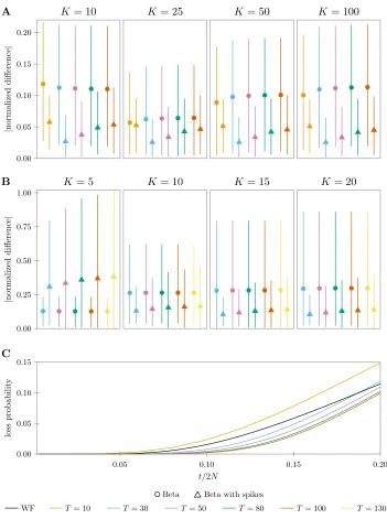
Figure 4 Inference of divergence times for the chimpanzee exome data. Thefigure shows box plots summarizing the inferred lengths using 50 data sets with 10,000 SNPs that were randomly sampled from the full data set. The corresponding tree branches are indicated at the top of each plot in black. The inferred lengths are plotted for beta (B), beta with spikes (BS), and Kim Tree (KT) (Gautier and Vitalis 2013). The nonsolid lines indicate the inferred lengths when running the methods on the full data set of 42,064 SNPs. The populations at the leaves are Eastern (E), Central (C), and Western (W). Each plot is scaled relative to the corresponding branch lengtht inferred by beta with spikes on the full data set. The limits of they-axis are set to

½t0:05;t1:5.

Figure 3 Inference of divergence times for simulation scenarios I (A) and II (B). Thefigure shows box plots summarizing the inferred lengths for the four branches of the tree, indicated at the top of each column in black. The inferred lengths are plotted for beta (B), beta with spikes (BS), and Kim Tree (KT) (Gautier and Vitalis 2013). The (true) simulated length of each branch is plotted as a horizontal line. Each plot is scaled relative to the corresponding simulated branch lengtht, with the limits of they-axis set to½t0:1;t1:5.

Kim Tree, implemented in Fortran. For the chimpanzee data set of 42,063 SNPs, beta with spikes ran in just under 5 min, while Kim Tree took almost an hour, even though Python 2.7 is a programming language that is less efficient than Fortran. We also note that the two inference methods are inherently different because here we used a numerical optimization pro-cedure, while Kim Tree uses a Bayesian MCMC approach. Additionally, unlike Kim Tree, beta with spikes is a recursive method, and its accuracy and speed depend on the number of iterations performed (seeFile S1for accuracy results for dif-ferent numbers of iterations).

Extensions

We end this section by discussing possible extensions of the beta with spikes approximation and how these can be used in inference problems. Throughout this paper, we assumed that the population size is constant. Given its recursive formula-tion, beta with spikes lends itself naturally to incorporating variable population size without any increase in computa-tional complexity. This can then be used for inference of population size backward in time, similar to methods relying on the coalescent with recombination (Li and Durbin 2011; Sheehanet al.2013; Schiffels and Durbin 2014). A recently published method (Liu and Fu 2015) illustrates that allele frequency data, summarized as site frequency spectra, can be used efficiently for inference of variable population size backward in time. Even though Liu and Fu (2015) assumed that sites are independent and did not use linkage informa-tion, their method can handle larger data sets than the method of Li and Durbin (2011), which leads to more accu-rate inference of population sizes for the recent past. The results obtained by Liu and Fu (2015) indicate that beta with spikes could be used successfully for such demographic inference.

Another extension of the presented approximation would be to incorporate selection, which is a nonlinear evolutionary pressure. In the recent years, there has been a great focus on inference of selection coefficients from time-series data under a Wright-Fisher model (Malaspinas et al.2012; Banket al.

2014; Steinrückenet al.2014; Follet al.2015; Terhorstet al.

2015). A newly developed statistical method aims at model-ing the evolution of multilocus alleles under a Wright-Fisher model with selection (Terhorstet al.2015) byfitting a multi-variate normal distribution from the first moments of the DAF. Using the approach of Terhorstet al.(2015) for moment calculation, beta with spikes can be extended to nonlinear evolutionary pressures. Terhorstet al.(2015) did not treat the loss and fixation probabilities. However, because selec-tion is expected to drive allele frequencies toward the bound-aries faster than pure genetic drift, including the explicit spikes becomes crucial.

Acknowledgments

It is a pleasure to thank Thomas Mailund for helpful discussions. We also thank the two anonymous reviewers

and the associate editor for their constructive suggestions and comments that helped to improve the manuscript. This work was supported, in part, by the European Research Council under the European Union’s Seventh Framework Program (FP7/20072013, ERC grant number 311341) and the Danish Research Council (grant number DFF-4002-00382).

Literature Cited

Abramowitz, M., and I. A. Stegun, 1964 Handbook of Mathemat-ical Functions: With Formulas,Graphs,and Mathematical Tables. Dover Publications, Mineola, NY.

Balding, D. J., and R. A. Nichols, 1995 A method for quantifying differentiation between populations at multiallelic loci and its implications for investigating identity and paternity. Genetica 96: 3–12.

Balding, D. J., and R. A. Nichols, 1997 Significant genetic corre-lations among Caucasians at forensic DNA loci. Heredity 78: 583–589.

Bank, C., G. B. Ewing, A. Ferrer-Admettla, M. Foll, and J. D. Jensen, 2014 Thinking too positive? Revisiting current methods of population genetic selection inference. Trends Genet. 30: 540– 546.

Bataillon, T., J. Duan, C. Hvilsom, X. Jin, Y. Li et al., 2015 Inference of purifying and positive selection in three sub-species of chimpanzees (Pan troglodytes) from exome sequenc-ing. Genome Biol. Evol. 7: 1122_–1132.

Coop, G., D. Witonsky, A. Di Rienzo, and J. K. Pritchard, 2010 Using environmental correlations to identify loci under-lying local adaptation. Genetics 185: 1411–1423.

Crow, J., and M. Kimura, 1956 Some genetic problems in natural populations, pp. 1–22 inProceedings of the Third Berkeley Sym-posium on Mathematical Statistics and Probability, Vol. 4. Uni-versity of California Press, Oakland, CA.

Crow, J. F., and M. Kimura, 1970 An Introduction to Population Genetics Theory. Harper & Row, New York.

Ewens, W. J., 2004 Mathematical Population Genetics 1: Theoret-ical Introduction, Vol. 27. Springer, New York.

Felsenstein, J., 1981 Evolutionary trees from DNA sequences: a maximum likelihood approach. J. Mol. Evol. 17: 368–376. Foll, M., H. Shim, and J. D. Jensen, 2015 WFABC: a Wright-Fisher

ABC-based approach for inferring effective population sizes and selection coefficients from time-sampled data. Mol. Ecol. Resour. 15: 87_–98.

Gautier, M., T. D. Hocking, and J.-L. Foulley, 2010 A Bayesian outlier criterion to detect SNPs under selection in large data sets. PLoS One 5: e11913.

Gautier, M., and R. Vitalis, 2013 Inferring population histories using genome-wide allele frequency data. Mol. Biol. Evol. 30: 654–668.

Gudbjartsson, D. F., H. Helgason, S. A. Gudjonsson, F. Zink, A. Oddsonet al., 2015 Large-scale whole-genome sequencing of the Icelandic population. Nat. Genet. 47: 435–444.

Hoban, S., G. Bertorelle, and O. E. Gaggiotti, 2012 Computer simulations: tools for population and evolutionary genetics. Nat. Rev. Genet. 13: 110–122.

Kimura, M., 1955 Solution of a process of random genetic drift with a continuous model. Proc. Natl. Acad. Sci. USA 41: 144. Kimura, M., 1964 Diffusion models in population genetics. J.

Appl. Probab. 1: 177–232.

Li, H., and R. Durbin, 2011 Inference of human population history from individual whole-genome sequences. Nature 475: 493_– 496.

Liu, X., and Y.-X. Fu, 2015 Exploring population size changes using SNP frequency spectra. Nat. Genet. 47: 555–559. Malaspinas, A.-S., O. Malaspinas, S. N. Evans, and M. Slatkin,

2012 Estimating allele age and selection coefficient from time-serial data. Genetics 192: 599–607.

McKane, A., and D. Waxman, 2007 Singular solutions of the dif-fusion equation of population genetics. J. Theor. Biol. 247: 849– 858.

Nicholson, G., A. V. Smith, F. Jónsson, Ó. Gústafsson, K. Stefánsson

et al., 2002 Assessing population differentiation and isolation from single-nucleotide polymorphism data. J. R. Stat. Soc. Se-ries B Stat. Methodol. 64: 695_–715.

Pickrell, J. K., and J. K. Pritchard, 2012 Inference of population splits and mixtures from genome-wide allele frequency data. PLoS Genet. 8: e1002967.

Romiguier, J., P. Gayral, M. Ballenghien, A. Bernard, V. Cahais

et al., 2014 Comparative population genomics in animals un-covers the determinants of genetic diversity. Nature 515: 261– 263.

Rosenberg, N. A., and M. Nordborg, 2002 Genealogical trees, co-alescent theory and the analysis of genetic polymorphisms. Nat. Rev. Genet. 3: 380–390.

Schiffels, S., and R. Durbin, 2014 Inferring human population size and separation history from multiple genome sequences. Nat. Genet. 46: 919–925.

Sheehan, S., K. Harris, and Y. S. Song, 2013 Estimating variable effective population sizes from multiple genomes: a sequentially Markov conditional sampling distribution approach. Genetics 194: 647–662.

Sirén, J., 2012 Statistical models for inferring the structure and history of populations from genetic data. Ph.D. thesis, University of Helsinki.

Sirén, J., P. Marttinen, and J. Corander, 2011 Reconstructing pop-ulation histories from single nucleotide polymorphism data. Mol. Biol. Evol. 28: 673–683.

Song, Y. S., and M. Steinrücken, 2012 A simple method forfi nd-ing explicit analytic transition densities of diffusion processes with general diploid selection. Genetics 190: 1117–1129. Steinrücken, M., A. Bhaskar, and Y. S. Song, 2014 A novel spectral

method for inferring general diploid selection from time series genetic data. Ann. Appl. Stat. 8: 2203.

Steinrücken, M., Y. R. Wang, and Y. S. Song, 2013 An explicit transition density expansion for a multiallelic Wright-Fisher dif-fusion with general diploid selection. Theor. Popul. Biol. 83: 1–14.

Terhorst, J., C. Schlötterer, and Y. S. Song, 2015 Multilocus anal-ysis of genomic time series data from experimental evolution. PLoS Genet. 11: e1005069.

Waxman, D., 2011 A compact result for the time-dependent prob-ability offixation at a neutral locus. J. Theor. Biol. 274: 131– 135.

Wright, S., 1945 The differential equation of the distribution of gene frequencies. Proc. Natl. Acad. Sci. USA 31: 382.

Zhao, L., X. Yue, and D. Waxman, 2013 Complete numerical so-lution of the diffusion equation of random genetic drift. Genetics 194: 973–985.

Communicating editor: Y. S. Song

GENETICS

Supporting Information

www.genetics.org/lookup/suppl/doi:10.1534/genetics.115.179606/-/DC1

Inference Under a Wright-Fisher Model Using an

Accurate Beta Approximation

Paula Tataru, Thomas Bataillon, and Asger Hobolth

Inference under a Wright-Fisher model

using an accurate beta approximation

Supporting Material

Paula Tataru

∗

, Thomas Bataillon

∗

, and Asger Hobolth

∗

Contents

Conditional mean and variance

2

Derivation of mean and variance of

X

t

2

Derivation of loss and fixation probabilities of

X

t

5

Approximation for small

a

and

b

7

Approximation for large

N

7

Parameter scaling

9

Discretization of beta and beta with spikes

9

Numerical accuracy of the beta and beta with spikes models

10

Likelihood calculation on a tree

10

Full data

11

Polymorphic data

12

The DAF at the root

13

Inference of divergence times: a simulation study

14

∗

_{Bioinformatics Research Centre, Aarhus University, Aarhus, 8000, Denmark}

Conditional mean and variance

If

X

is a discrete random variable with values between 0 and 1, its mean conditional on

X

_{6∈ {}

0

,

1

_}

can be calculated as follows

E

[

X

_|

X

_{6∈ {}

0

,

1

_}

] =

X

x:x6∈{0,1}

x

_·

_P

(

X

=

x

_|

X

_{6∈ {}

0

,

1

_}

)

=

X

x:x6∈{0,1}

x

_·

P

(

X

=

x

)

P

(

X

_{6∈ {}

0

,

1

_}

)

=

1

P

(

X

_{6∈ {}

0

,

1

_}

)

X

x:x6∈{0,1}

x

_·

_P

(

X

=

x

)

=

1

P

(

X

_{6∈ {}

0

,

1

_}

)

(

E

[

X

]

−

0

·

P

(

X

= 0 )

−

1

·

P

(

X

= 1 ))

=

E

[

X

]

−

P

(

X

= 1 )

P

(

X

_{6∈ {}

0

,

1

_}

)

.

Similarly, we obtain

E

X

2

_|

X

_{6∈ {}

0

,

1

_}

=

E

[

X

2

_]

₋

P

(

X

= 1 )

P

(

X

_{6∈ {}

0

,

1

_}

)

=

Var (

X

) +

E

[

X

]

2

−

P

(

X

= 1 )

P

(

X

_{6∈ {}

0

,

1

_}

)

,

from which

Var (

X

_|

X

_{6∈ {}

0

,

1

_}

) =

_E

X

2

_|

X

_{6∈ {}

0

,

1

_}

₋

_E

[

X

_|

X

_{6∈ {}

0

,

1

_}

]

2

=

Var (

X

) +

E

[

X

]

2

−

P

(

X

= 1 )

P

(

X

_{6∈ {}

0

,

1

_}

)

−

E

[

X

|

X

6∈ {

0

,

1

}

]

2

.

Derivation of mean and variance of

X

_t

To calculate the mean and variance of

X

t

under the Wright-Fisher model, we rely on the

laws of total mean and variance, respectively. Recall that

X

t

=

Z

t

/

2

N

and

Z

t+1

|

Z

t

=

z

t

∼

Bin(2

N, g

(

x

t

))

,

where

x

t

=

z

t

/

2

N

. The evolutionary pressures

g

(

x

) satisfy that 0

≤

g

(

x

)

≤

1 for all

0

_≤

x

_≤

1. In the following,

g

is a linear function in the allele frequency,

g

(

x

) = (1

₋

a

)

x

+

b

.

2

The parameters

a

and

b

satisfy that 0

_≤

b

_≤

a <

1 and typically,

a <<

1. We note that if

a

= 0, then

b

= 0. In the derivations below, we condition implicitly on

X

0

=

x

0

, population

size 2

N

and evolutionary pressures.

Let us start with the mean and variance of

X

t+1

conditional on

X

t

=

x

t

, given by

E

[

X

t+1

|

X

t

=

x

t

] =

1

2

N

E

[

Z

t+1

|

Z

t

=

z

t

]

=

1

2

N

2

N g

(

x

t

)

=

g

(

x

t

)

,

Var (

X

t+1

|

X

t

=

x

t

) =

1

4

N

2

Var (

Z

t+1

|

Z

t

=

z

t

)

=

1

4

N

2

2

N g

(

x

t

) (1

−

g

(

x

t

))

=

1

2

N

g

(

x

t

) (1

−

g

(

x

t

))

.

First, using the law of total expectation, we have that

E

[

X

t

] =

E

[

E

[

X

t

|

X

t−1

] ]

=

_E

[

g

(

X

t−1

) ]

=

_E

[ (1

₋

a

)

X

t−1

+

b

]

= (1

₋

a

)

_E

[

X

t−1

] +

b

= (1

₋

a

)

_E

[

_E

[

X

t−1

|

X

t−2

] ] +

b

=

. . .

= (1

₋

a

)

t

x

0

+

b

t−1

X

i=0

(1

₋

a

)

i

.

When

a

=

b

= 0, the mean becomes

E

[

X

t

] =

x

0

.

If

a

₆

= 0,

t−1

X

i=0

(1

₋

a

)

i

=

1

−

(1

−

a

)

t

a

,

and this gives

E

[

X

t

] =

b

a

+ (1

−

a

)

t

x

0

−

b

a

.

We use a similar approach to determine the variance of

X

t

, this time relying on the law

of total variance

Var (

X

t

) =

E

[ Var (

X

t

|

X

t−1

) ] + Var (

E

[

X

t

|

X

t−1

] )

=

_E

1

2

N

g

(

X

t−1

) (1

−

g

(

X

t−1

))

+ Var (

g

(

X

t−1

) )

=

1

2

N

E

[

g

(

X

t−1

) ]

−

1

2

N

E

g

(

X

t−1

)

2

+ Var (

g

(

X

t−1

) )

=

1

2

N

E

[

g

(

X

t−1

) ]

−

1

2

N

Var (

g

(

X

t−1

) )

−

1

2

N

E

[

g

(

X

t−1

) ]

2

+ Var (

g

(

X

t−1

) )

=

1

2

N

E

[

g

(

X

t−1

) ] (1

−

E

[

g

(

X

t−1

) ]) +

1

₋

1

2

N

Var (

g

(

X

t−1

) )

=

1

2

N

E

[

X

t

] (1

−

E

[

X

t

]) +

1

₋

1

2

N

(1

₋

a

)

2

Var (

X

t−1

)

.

Iterating the above,

Var (

X

t

) =

1

2

N

t

X

i=1

(1

₋

a

)

2(t−i)

1

₋

1

2

N

t−i

E

[

X

i

] (1

−

E

[

X

i

])

.

Let us observe that, for any

c

,

1

2

N

t

X

i=1

(1

₋

a

)

c(t−i)

1

₋

1

2

N

t−i

=

1

2

N

·

1

₋

(1

₋

a

)

c t

1

₋

_2N1

t

1

₋

(1

₋

a

)

c

₁

₋

1

2N

=

1

−

(1

−

a

)

c t

₁

₋

1 2N

t

2

N

₋

(1

₋

a

)

c

₍₂

_N

₋

₁₎

.

When

a

=

b

= 0 and using

c

= 0 in the above, the variance becomes

Var (

X

t

) =

x

0

(1

−

x

0

)

"

1

₋

1

₋

1

2

N

t

#

.

If

a

₆

= 0,

E

[

X

i

] (1

−

E

[

X

i

]) =

b

a

1

₋

b

a

+

1

₋

2

b

a

(1

₋

a

)

i

x

0

−

b

a

−

(1

₋

a

)

2i

x

0

−

b

a

2

,

and using

c

= 1 and

c

= 2, respectively, we obtain the variance

Var (

X

t

) =

b

a

1

₋

b

a

1

2

N

t

X

i=1

(1

₋

a

)

2(t−i)

1

₋

1

2

N

t−i

+

1

₋

2

b

a

x

0

−

b

a

(1

₋

a

)

t

1

2

N

t

X

i=1

(1

₋

a

)

t−i

1

₋

1

2

N

t−i

−

x

0

−

b

a

2

(1

₋

a

)

2t

1

2

N

t

X

i=1

1

₋

1

2

N

t−i

=

b

a

1

₋

b

a

₁

₋

₍₁

₋

_a

₎

2t

₁

₋

1 2N

t

2

N

₋

(1

₋

a

)

2

₍₂

_N

₋

₁₎

+

1

₋

2

b

a

x

0

−

b

a

(1

₋

a

)

t

1

−

(1

−

a

)

t

₁

₋

1 2N

t

2

N

₋

(1

₋

a

) (2

N

₋

1)

−

x

0

−

b

a

2

(1

₋

a

)

2t

1

₋

1

₋

1

2

N

t

!

.

See the parameter scaling section for a comparison with the derivations obtained by

Sir´

en (2012). We note that Sir´

en (2012) relies on approximations resulting from the infinite

population limit, while the above equations hold for any population size.

The derivations for the mean and variance use the linearity of the evolutionary pressures

through the simplification that

E

[ (1

₋

a

)

X

t

+

b

] = (1

−

a

)

E

[

X

t

] +

b,

Var ( (1

₋

a

)

X

t

+

b

) = (1

−

a

)

2

Var (

X

t

)

.

When

g

(

x

) is a polynomial of higher order, such as in the case of selection, the derivation

requires higher moments of

X

t

, leading to an explosion in the moments needed and rendering

the above approach untractable in such situations.

Derivation of loss and fixation probabilities of

X

_t

To determine

_P

(

X

t+1

= 0 ) and

P

(

X

t+1

= 1 ), we use the law of total probability in an

approach similar to the above. Additionally, we rely on the approximation that

X

t

follows

a known

f

?

B

beta with spikes distribution to obtain

P

(

X

t+1

= 0 ) =

Z

1

0

P

(

X

t+1

= 0

|

X

t

=

x

)

·

f

B?

(

x

;

t

) d

x

=

_P

(

X

t+1

= 0

|

X

t

= 0 )

·

P

(

X

t

= 0 ) +

P

(

X

t+1

= 0

|

X

t

= 1 )

·

P

(

X

t

= 1 )

+

_P

(

X

t

6∈ {

0

,

1

}

)

·

Z

1

0

P

(

X

t+1

= 0

|

X

t

=

x

)

·

x

α?t−1

(1

−

x

)

βt?−1

B (

α

? t

, β

t?

)

d

x

=

_P

(

X

t

= 0 )

·

(1

−

g

(0))

2N

+

P

(

X

t

= 1 )

·

(1

−

g

(1))

2N

+

_P

(

X

t

6∈ {

0

,

1

}

)

·

Z

1

0

(1

₋

g

(

x

))

2N

_·

x

α?

t−1

(1

−

x

)

βt?−1

B (

α

? t

, β

t?

)

d

x,

where B (

α, β

) is the beta function.

To calculate the above integral for linear evolutionary pressures, we rely on the

hyper-geometric function. Let

2

F

1

(

−

m, b

;

c

;

z

) ((Erd´

elyi

et al.

1953), 2.1.3) be the hypergeometric

function for

m

_∈

_N

,

c, d

_∈

_R+

and

z

_∈

_R

, given by

2

F

1

(

−

m, c

;

c

+

d

;

z

) =

1

B (

c, d

)

Z

1

0

x

c−1

(1

₋

x

)

d−1

(1

₋

z x

)

m

d

x.

We have that (recall that 0

_≤

b <

1)

Z

1

0

(1

₋

g

(

x

))

2N

_·

x

α?

t−1

(1

−

x

)

βt?−1

B (

α

? t

, β

t?

)

d

x

=

1

B (

α

? t

, β

t?

)

Z

1

0

((1

₋

b

)

₋

(1

₋

a

)

x

)

2N

x

α?t−1

₍₁

−

_x

₎

βt?−1

_d

_x

=

(1

−

b

)

2N

B (

α

? t

, β

t?

)

Z

1

0

1

₋

1

−

a

1

₋

b

x

2N

x

α?t−1

₍₁

−

_x

₎

β?t−1

_d

_x

= (1

₋

b

)

2N2

F

1

−

2

N, α

?_t

;

α

_t?

+

β

_t?

;

1

−

a

1

₋

b

,

leading to the full expression for the loss probability

P

(

X

t+1

= 0 ) =

P

(

X

t

= 0 )

·

(1

−

b

)

2N

+

P

(

X

t

= 1 )

·

(

a

−

b

)

2N

+

_P

(

X

t

6∈ {

0

,

1

}

)

·

(1

−

b

)

2N

·

2

F

1

−

2

N, α

?_t

;

α

_t?

+

β

_t?

;

1

−

a

1

₋

b

.

Similarly, for

b

₆

= 0 (if

b

= 0, see below), we obtain the fixation probability

P

(

X

t+1

= 1 ) =

P

(

X

t

= 0 )

·

b

2N

+

P

(

X

t

= 1 )

·

(1

−

a

+

b

)

2N

+

_P

(

X

t

6∈ {

0

,

1

}

)

·

b

2N

·

2

F

1

−

2

N, α

?_t

;

α

_t?

+

β

_t?

;

₋

1

−

a

b

.

Approximation for small

a

and

b

The hypergeometric function can be cumbersome and

slow to evaluate. Typically the parameters

a

and

b

are small and we can use that

1

₋

g

(

x

) = (1

₋

a

)(1

₋

x

) +

a

₋

b

_≈

(1

₋

a

)(1

₋

x

)

,

g

(

x

) = (1

₋

a

)

x

+

b

_≈

(1

₋

a

)

x,

to more easily reduce the above integrals to

Z

1

0

(1

₋

g

(

x

))

2N

_·

x

α?

t−1

(1

−

x

)

βt?−1

B (

α

? t

, β

t?

)

d

x

_≈

(1

₋

a

)

2N

_·

Z

1

0

x

α?

t−1

(1

−

x

)

βt?+2N−1

B (

α

? t

, β

t?

)

d

x

= (1

₋

a

)

2N

_·

B (

α

?

t

, β

t?

+ 2

N

)

B (

α

?

t

, β

t?

)

,

Z

1

0

g

(

x

)

2N

_·

x

α?

t−1

(1

−

x

)

βt?−1

B (

α

? t

, β

t?

)

d

x

_≈

(1

₋

a

)

2N

_·

B (

α

?

t

+ 2

N, β

t?

)

B (

α

?

t

, β

t?

)

,

from which

P

(

X

t+1

= 0 )

≈

P

(

X

t

= 0 )

·

(1

−

b

)

2N

+

P

(

X

t

= 1 )

·

(

a

−

b

)

2N

+

_P

(

X

t

6∈ {

0

,

1

}

)

·

(1

−

a

)

2N

·

B (

α

?

t

, β

t?

+ 2

N

)

B (

α

?

t

, β

t?

)

,

P

(

X

t+1

= 1 )

≈

P

(

X

t

= 0 )

·

b

2N

+

P

(

X

t

= 1 )

·

(1

−

a

+

b

)

2N

+

_P

(

X

t

6∈ {

0

,

1

}

)

·

(1

−

a

)

2N

·

B (

α

?_t

+ 2

N, β

_t?

)

B (

α

?

t

, β

t?

)

.

For the results reported in the main text and below (in numerical accuracy and inference

of divergence times sections), we used the above approximation for small

a

and

b

.

Approximation for large

N

A widely used assumption in the derivations based on the

Wright-Fisher model, such as the diffusion limit, is that the population size

N

is large, and

a

and

b

are small such that

lim

N→∞

2

N a

=

A,

N

lim

→∞

2

N b

=

B.

Additionally, the time is scaled by the population size,

τ

=

t/

2

N

. We set ∆ = 1

/

2

N

.

Because

a

and

b

are small, we build on the previous approximation.

Let Γ(

c

) be the Gamma function and note that, for large

N

((Erd´

elyi

et al.

1953), 1.18),

Γ(

N

+

c

)

Γ(

N

+

c

+

d

)

≈

1

N

d

1

₋

d

(

c

+ 2

d

−

1)

2

N

.

We then have

B (

α

?

t

, β

t?

+ 2

N

)

B (

α

?

t

, β

t?

)

=

Γ(

α

?

t

) Γ(

β

t?

+ 2

N

)

Γ(

α

?

t

+

β

t?

+ 2

N

)

·

Γ(

α

? t

+

β

t?

)

Γ(

α

?

t

) Γ(

β

t?

)

=

Γ(

α

? t

+

β

t?

)

Γ(

β

?

t

)

·

Γ(2

N

+

β

? t

)

Γ(2

N

+

α

?

t

+

β

t?

)

≈

Γ(

α

? t

+

β

t?

)

Γ(

β

? t

)

·

1

2

N

α?t

·

1

₋

α

?

t

(2

α

?t

+

β

t?

−

1)

4

N

=

Γ(

α

? t

+

β

t?

)

Γ(

β

?

t

)

·

∆

α?t

·

1

₋

1

2

∆

α

?

t

(2

α

?t

+

β

?t

−

1)

,

and, similarly,

B (

α

?_t

+ 2

N, β

_t?

)

B (

α

?

t

, β

t?

)

≈

Γ(

α

? t

+

β

t?

)

Γ(

α

?

t

)

·

∆

β?t

·

1

₋

1

2

∆

β

? t

(

α

? t

+ 2

β

? t

−

1)

.

Using that

lim

N→∞

(1

−

a

)

2N

₌

_e

−A

_,

_lim

N→∞

(1

−

b

)

2N

₌

_e

−B

_,

lim

N→∞

(1

−

a

+

b

)

2N

=

e

−(A−B)

,

lim

N→∞

(

a

−

b

)

2N

= 0

,

we obtain the recursion in scaled time for loss and fixation probabilities to be

P

(

X

τ+∆

= 0 )

≈

P

(

X

τ

= 0 )

·

e

−B

+

_P

(

X

τ

6∈ {

0

,

1

}

)

·

e

−A

·

Γ(

α

? τ

+

β

τ?

)

Γ(

β

? τ

)

·

∆

α?τ

·

1

₋

1

2

∆

α

? τ

(2

α

? τ

+

β

? τ

−

1)

,

P

(

X

τ+∆

= 1 )

≈

P

(

X

τ

= 1 )

·

e

−(A−B)

+

_P

(

X

τ

6∈ {

0

,

1

}

)

·

e

−A

·

Γ(

α

? τ

+

β

τ?

)

Γ(

α

? τ

)

·

∆

βτ?

·

1

₋

1

2

∆

β

? τ

(

α

? τ

+ 2

β

? τ

−

1)

.