Effect of Local Bed Hydrodynamics on the Distribution of Liquid in a Fluidized Bed

(1)

Western University Western University

Scholarship@Western

Electronic Thesis and Dissertation Repository

9-16-2016 12:00 AM

Effect of Local Bed Hydrodynamics on the Distribution of Liquid in

a Fluidized Bed

Lingchao Li

The University of Western Ontario

Supervisor Franco Berruti

The University of Western Ontario Joint Supervisor Cedric Briens

The University of Western Ontario

Graduate Program in Chemical and Biochemical Engineering

A thesis submitted in partial fulfillment of the requirements for the degree in Master of Engineering Science

Follow this and additional works at: https://ir.lib.uwo.ca/etd Part of the Other Chemical Engineering Commons

Recommended Citation Recommended Citation

Li, Lingchao, "Effect of Local Bed Hydrodynamics on the Distribution of Liquid in a Fluidized Bed" (2016). Electronic Thesis and Dissertation Repository. 4120.

https://ir.lib.uwo.ca/etd/4120

This Dissertation/Thesis is brought to you for free and open access by Scholarship@Western. It has been accepted for inclusion in Electronic Thesis and Dissertation Repository by an authorized administrator of

(2)

i

Abstract

In an industrial Fluid CokerTM, liquid bitumen is injected into a bed of hot coke particles through spray nozzles, grouped in several banks at different vertical positions. The main objective of this thesis is to determine whether significant improvements in liquid-solid contact could be achieved by optimizing the location of the spray nozzles.

In the coker regions where bitumen is injected, the gas is a mixture of product vapors and steam. Steam introduced at different levels rises through the coker: the stripping steam is injected near the bottom, then the attrition steam above the stripper and finally the bitumen atomization steam. As a result, the cross-sectional averaged gas velocity greatly varies vertically, from the lowest spray bank to the highest spray bank. In addition, there are large radial variations in gas velocity, as gas bubbles tend to concentrate in the central region of the bed.

In this study, the impacts of gas velocity and uneven gas distribution on liquid-solid contact were investigated. The effects of spray pulsations and atomization gas flowrate on liquid distribution were also studied. Effects of bed hydrodynamics on the initial liquid distribution and on the subsequent drying were studied separately.

The results indicate that jet pulsations or increasing the atomization gas flowrate improve the liquid distribution. Large improvements in liquid distribution were achieved by increasing the superficial gas velocity and also increasing the gas velocity at the end of the spray jet cavity, for all types of spray jets, pulsating or non-pulsating.

(3)

ii

Acknowledgement

I would like to thank Dr. Cedric Briens and Dr. Franco Berruti for their support and mentorship during these past two years. The chance they offered to work in an industrially related program is greatly appreciated.

I would also like to thank the National Science and Engineering Research Council of Canada, Syncrude Canada and ExxonMobil for their generous financial support. Special thanks to Dr. Jennifer McMillan for her instructions and advice throughout my research.

I would like to thank all ICFAR staff members for their technical and administrative support. They made a very friendly working environment and a highly efficient team. I would like to thank Liliana Pardo for introducing me to the high velocity fluidized bed at the beginning of my program. I would also like to thank Francisco Sanchez for his help with my project and all advice as a sincere friend.

(4)

iii

List of tables

Table 4-1 Mass of solids entrained in left and right internal cyclones at different gas distributions ... 50

Table 5-1 Linear velocities of liquid and atomization gas in different sizes of conduits ... 57

(9)

viii

List of figures

Figure 1.1 Process flow diagram of fluid coking [1] ... 1

Figure 1.2 Mechanism of agglomerate formation in a gas-solid fluidized bed [11] ... 4

Figure 1.3 Schematic of granulation processes [12] ... 5

Figure 1.4 Schematic diagram of feed-coke interaction [13] ... 6

Figure 2.1 Schematic diagram of high gas velocity fluidized bed (front view) ... 10

Figure 2.2 Schematic diagram of high gas velocity fluidized bed (lateral view) ... 11

Figure 2.3 Picture of the sparger ... 12

Figure 2.4 Schematic diagram of the sparger in the fluidized bed. The direction of gas entering the fluidized bed is parallel to the angled wall. ... 12

Figure 2.5 Diagram of TEB spray nozzle ... 13

Figure 2.6 Schematic diagram of injection system ... 13

Figure 2.7 Size distribution of silica sand for experiments ... 14

Figure 2.8 The electrical circuit system for conductance measurement ... 15

Figure 2.9 Calibration curve for blue dye ... 17

Figure 2.10 A single pixel in the original photo of the spray ... 19

Figure 2.11 A single pixel in the photo of the spray transferred into gray scale ... 19

Figure 2.12 Amount of pixels for each Gray Intensity for pure background ... 20

Figure 2.13 Amount of pixels for each Gray Intensity ... 21

(10)

ix

Figure 2.15 Geometry of jet expansion angle calculation ... 23

Figure 2.16 Photo of the jet, GLR=1%, FL=23.4 g/s ... 23

Figure 2.17 Gray intensity values in the pixels where x=100, GLR=1% when x=100, y represents the vertical locations of pixels. ... 24

Figure 3.1 Conductance signal for injection of 180 g H2O at room temperature ... 26

Figure 3.2 Conductance signal for injection of 150 g Gum Arabic solution at 130 °C ... 27

Figure 3.3 Cumulative weight percentage of agglomerates in bed solid mass for various Vgi while Vgd is constant at 0.18 m/s ... 28

Figure 3.4 The effect of Vgi on amount of macro and micro agglomerates while Vgd is constant at 0.18 m/s ... 29

Figure 3.5 Cumulative fraction of water trapped in agglomerates various Vgi while Vgd is constant at 0.18 m/s... 30

Figure 3.6 Effect of Vgi on the total amount of free moisture ... 31

Figure 3.7 Initial L/S ratio in macro and micro agglomerates at various Vgi at constant Vgd=0.18 m/s ... 32

Figure 3.8 Effect of increasing Vgd on the amount of agglomerates at different Vgi (0.18, 2.2 m/s) ... 33

Figure 3.9Effect of Vgd on liquid to solid ratio when Vgi= 0.18 m/s and Vgi= 2.2 m/s ... 34

Figure 3.10 Effect of Vgd on amount of agglomerates when Vgi= 0.18 m/s and Vgi=2.2 m/s ... 35

Figure 4.1 Schematic diagram of triboelectricity measurement system ... 37

Figure 4.2 Top view of the locations of the 20 sonic nozzles... 37

(11)

x

Figure 4.4 Raw signal of triboelectricity measurement, superficial gas velocity 1m/s ... 40

Figure 4.5 Power spectra of triboelectricity measurement for a low bubble gas flowrate ... 41

Figure 4.6 Power spectra of triboelectricity measurement for a high bubble gas flowrate ... 41

Figure 4.7 Correlation between the real average volumetric flux of bubble gas and the average volumetric flux calculated... 43

Figure 4.8 Group 1 gas distributions, (a) 0.6-0.4 m/s, (b) 0.1-0.9 m/s, (c) 0.9-0.1 m/s ... 44

Figure 4.9 Profiles of gas bubble flow for Group 1 gas distributions. (The profile was measured without the jet) ... 45

Figure 4.11 Profiles of gas bubble flow for Group 2 gas distributions... 46

Figure 4.13 Profiles of gas bubble flow for Group 3 gas distributions... 47

Figure 4.14 Summary of bubble gas flow radial profiles of various gas distributions ... 48

Figure 4.15 schematic diagram of the high gas velocity fluidized bed ... 49

Figure 4.16 Fraction of free moisture in mass of liquid injected (data for even distribution is obtained from section 3.2.2) ... 51

Figure 4.17 weight percentage of agglomerates in bed mass ... 52

Figure 4.18 liquid to solid ratio in agglomerates for gas distributions ... 53

Figure 5.1 Injection system for pulsating spray ... 55

(12)

xi

Figure 5.3 Flow pattern map of Taitel and Dukler [30]. The dotted line refers to the modified transition line between the intermittent and annular regimes, as proposed by Barnea et al [31]. 56

Figure 5.4 Pictures of spray (pulsating spray, t=0 is the beginning of injection) ... 58

Figure 5.5 Stability analysis for pulsating spray, GLR=2.2%, FL=21.4 g/s ... 59

Figure 5.6 Stability analysis for stable spray GLR=2.2%, FL=21.4 g/s ... 60

Figure 5.7 Cumulative Wt% of agglomerates in bed mass GLR=2.2%, FL=21.4 g/s (two experiments for each condition)... 61

Figure 5.8 Initial L/S ratio in agglomerates (g/g) GLR=2.2%, FL=21.4 g/s ... 62

Figure 5.9 Cumulative fraction of water trapped in agglomerates GLR=2.2%, FL=21.4 g/s ... 62

Figure 5.10 Cumulative Wt% of agglomerates in bed mass GLR=2.2%, FL=21.4 g/s ... 63

Figure 5.12 Cumulative fraction of water trapped in agglomerates GLR=2.2%, FL=21.4 g/s ... 64

Figure 5.15 Amount of water trapped in agglomerates GLR=2.2%, FL=21.4 g/s ... 66

(13)

xii

Figure 5.20 Cumulative weight fraction of water trapped in agglomerates, GLR=2.2%, FL=21.4

g/s ... 70

Figure 5.21 Stability analysis for open air spray at various GLRs, FL=23.4 g/s ... 71

Figure 5.22 Jet expansion angle for sprays of different GLRs in the open air ... 72

Figure 5.23 Free moisture fraction in the water injected for different GLRs, FL=23.4 g/s ... 73

Figure 5.24 Cumulative fraction of water trapped in agglomerates in total amount of water injected for different GLRs, FL=23.4 g/s ... 73

Figure 5.25 Total fraction of agglomerates in bed mass for different GLRs, FL=23.4 g/s ... 74

Figure 5.26 Cumulative wt% of agglomerates in bed mass for different GLRs, FL=23.4 g/s ... 75

(14)

xiii

Lists of symbols

daggl Diameter of agglomerates (μm)

dp Particle diameter (μm)

f Average frequency

GLR Gas to liquid ratio

i Gray intensity

Ljet Jet penetration distance (m)

md Mass of dye (g)

mGA Mass of Gum Arabic (g)

mp Mass of particles trapped in agglomerates (kg)

mR Representative sample taken from m<600μm(g)

msand Total mass of individual particles and agglomerates (g)

mμaggl, i Total mass of micro-agglomerates in the bed for a given size cut (g)

mμaggl, Ri Mass of micro-agglomerates in the sample for a given size cut (g)

m<600μm Bed mass after removal of agglomerates larger than 600 μm

P Power spectral density

qbi local volumetric flux of bubble gas, m3/ (s∙m2)

qb

̅̅̅ Cross-sectional average volumetric flux of bubble gas, m3_{/ (s}_∙_m2₎

(15)

xiv ULS Linear velocity of liquid in the conduit

umf Minimum fluidization velocity

xf Fraction of particles smaller than 355 µm in msand

xbed Fraction of particles smaller than 355 µm in initial particle size distribution (PSD)

Vg Gas velocity, m/s

Vgi Superficial velocity during liquid injection, m/s

Vgd Superficial velocity during drying, m/s

α Coefficient for correlation of power spectral density, frequency and local volumetric

flux of bubble gas flow

β Coefficient for correlation of power spectral density, frequency and local volumetric

γ Coefficient for correlation of power spectral density, frequency and local volumetric

λ Local cross-sectional area for volumetric flux of bubble gas, m2

(16)

1

Introduction

The present work addresses factors that could help improve the distribution of liquid injected into a solid-gas fluidized bed. Good liquid-solid contact is crucial to maintain good operability and maximize the yield of valuable liquid in Fluid CokersTM. The formation of undesired agglomerates needs to be minimized for better mass and heat transfer.

The key motivation of this study is to have a better understanding of impacts of different bed hydrodynamics on liquid distribution.

1.1 Fluid Coking

TM

Figure 0.1 Process flow diagram of fluid coking [1]

Canada’s oil sands are the world’s largest known concentration of bitumen. The current estimate

of the ultimately recoverable volume represents only 12 percent of the ultimate volume of

(17)

2

Figure 1.1 provides a schematic diagram of the Fluid CokingTM process. A Fluid Coking unit is made up of 2 vessels, the coking vessel and the burner vessel. Liquid feedstocks can be heavy or reduced crudes or vacuum bottoms containing constituents that cannot be vaporized without decomposition. Feeds typically have an API between 0 to 20° and a Conradson carbon content of circa 5 to 40 weight percent. Liquid feedstock atomized with steam is sprayed into the reactor (coking vessel) after being preheated to 200 to 400 °C. It is very important to distribute the feed quickly and uniformly over particles in the bed. Spray nozzles are located at multiple points both circumferentially and vertically to avoid excessive concentration of liquid in a part of the bed. The average superficial velocity of the rising gases varies with height and is usually

between 0.3 and 0.9 m/s. The temperature in the reactor is preferably maintained between 480 °C to 540 °C while the gauge pressure is between 0 to 3.5 bar. [3]

In the fluid bed reactor, the feed is converted to hot hydrocarbon vapor, permanent gases and solid coke. The gas and vapors pass through cyclones where most of the entrained particles are removed. Then the vapors enter a scrubber section in which remaining particles are removed and heavy liquids are condensed. At the base of the reactor, coke particles flow through the stripping section and interstitial product vapors are removed by a stripping gas, e.g. steam. The coke particles flow down through a stand-pipe then up though a riser to the burner. A portion of the coke particles are burned with air to produce enough heat for the process. The remaining,

reheated particles are then transported back to the reactor to supply the heat required for reaction. Net coke is removed as product coke. [4]

1.2 Bed hydrodynamics

In a Fluid Coker, superficial gas velocity increases with increasing height due to the steam from the stripper section and attrition nozzles, and the gases and vapors from the pyrolysis of feed injected at different levels.

(18)

3

voidage increases gradually from the wall to the center of the bed without a sharp transition from the annular region and the core region. This means that in the core region the gas velocity is higher than the cross-sectional average superficial gas velocity at the same height.

Mohagheghi et al. [6] used a conductance method to investigate the effect of local

hydrodynamics on liquid distribution in a gas-solid fluidized bed, and found that a higher fluidization velocity during liquid injection is beneficial for liquid-solid contact.

Pougatch et al. [7] developed a novel mathematical model to describe the spray jet and its contact with solid particles in a fluidized bed. Through analysis they found that increasing gas velocity improves liquid-solid contact in the region far from the tip of the nozzle. Increasing the gas velocity has no measurable influence on liquid-solid contact in the region near the nozzle tip.

Morales et al. [8] conducted injections with a liquid solution which uses PlexiglasTM as binder to investigate the effect bed hydrodynamics on liquid distribution. They found that increasing the gas velocity in fluidized bed reduces the total amount of agglomerates. A higher gas velocity increases the amount of smaller, micro agglomerates but decreases the amount of larger, macro agglomerates, which are more problematic in the industrial process. However, the impacts of gas velocity on initial liquid distribution and on agglomerate breakage were not separated.

Weber et al. [9] investigated various factors that can possibly affect the agglomerate behavior in a fluidized bed. They found that agglomerate destruction is a complex process which is

determined by several parameters, i.e. superficial gas velocity, initial agglomerate size, liquid concentration and liquid physical properties. Increasing the superficial velocity can switch the agglomerate size reduction mechanism to the more effective fragmentation regime. In

accordance with this conclusion, Mohagheghi[6] utilized the capacitance method to confirm that increasing the gas velocity after liquid injection accelerates the breakage of agglomerates.

(19)

4

1.3 Liquid distribution and agglomeration

Particle agglomeration occurs when liquid is sprayed into a gas-solid fluidized bed. Undesired agglomerates in a Fluid Coker need to be minimized for better mass and heat transfer.

Bruhns and Werther [11] proposed a model for the mechanism of the injection of liquid reactants into a fluidized bed reactor. When the liquid is sprayed into the fluidized reactor, no

instantaneous liquid evaporation occurs at the nozzle tip even though the bed temperature is higher than the boiling point of the liquid. The liquid jet penetrates the bed and wets the particles entrained into the region of liquid – solid interaction. Agglomerates formed in this region are then transported into other parts of the bed. Due to the shear forces in the fluidized bed, resulting from gas bubbles, and the agglomerates are susceptible to breakup.

Figure 0.2 Mechanism of agglomerate formation in a gas-solid fluidized bed [11]

(20)

5

Figure 0.3 Schematic of granulation processes [12]

1. Wetting and nucleation. The liquid binder is sprayed into the fluidized bed and is distributed on the particles to give a distribution of nuclei granules;

2. Consolidation and growth. Granules collide with other granules, dry feed powder or the equipment which leads to granule compaction and growth;

3. Attrition and breakage. Wet or dried agglomerates break up due to impact, erosion or compaction.

(21)

6

Figure 0.4 Schematic diagram of feed-coke interaction [13]

In the first step, the liquid feed is atomized and introduced into the fluidized bed. Secondly, a feed drop entering the bed collides with several particles since the particles are smaller. Particles wrapped by the drop form a wet granule. In the last step, due to gas velocities in the fluid bed (0.3-1.5 m/s), the granule tends to be broken up by shear forces. This mechanism results in uniformly coated particles. The thickness of liquid film depends on the local voidage of the fluidized bed and the liquid fraction in the void volume.

1.4 Spray performance

1.4.1 Atomization gas to liquid ratio (GLR)

Farkhondehkavaki et al. [14] used various methods to characterize the amount of free

(22)

7

ZirGachian et al. [16] applied a novel measurement method employing electrical conductance in a large scale fluidized bed of 7 tons of silica sand. They conducted liquid injections with an industrial scale TEB nozzle. They showed that raising the GLR from 0 % to 5.59 % can greatly improve the efficiency of liquid-solid contact.

Portoghese et al. [17] developed a new method to characterize the efficiency of the injection of liquid sprayed into a fluidized bed. A Nozzle Performance Index (NPI) was derived from

triboelectric signals for nozzles injecting air-atomized water into a gas–solid fluidized bed. Using this method, they also found that increasing the GLR would be beneficial to liquid distribution. The optimal GLR, however, depends on the nozzle size and operating liquid flowrate. It is also suggested that a better jet-bed interaction is obtained from 2 factors:

1. Finer liquid droplets at the nozzle tip

2. A higher rate of solid entrainment into the jet cavity caused by a larger expansion angle of the gas-liquid jet

Leach et al. [18] utilized a conductance method to characterize the performance of various atomizing feed nozzles at different GLRs. For the patented TEB nozzle which is widely used in the industrial process, it is reported that an optimal GLR exists at around 2.5 %. Increasing the GLR past 2.5% deteriorates the quality of liquid-solid contact. Leach et al. [18] also found that the impact of GLR is completely different for nozzles of different geometry.

Mohagheghi et al. [6] applied a new capacitance measurement method to characterize the liquid distribution in a fluidized bed. The results indicated as well that a higher GLR of the feed nozzle contributes to better contact between atomized liquid and fluidized particles.

1.4.2 Spray stability

(23)

8

Sabouni, et al. [19] utilized a solenoid valve to introduce fluctuations of well-defined frequency to an atomized gas-liquid spray. They found that at three different GLRs, jet fluctuation

improved liquid distribution. They also confirmed the significantly beneficial effect of pulsations on liquid-solid contact over a range of operating conditions i.e. different liquid flow rates, gas properties and spray nozzle geometry.

Later, the authors [20] created a plug flow before the gas-liquid mixture exited the nozzle tip. This resulted in a spray pulsation in the fluidized bed. The results indicated that pulsations can improve liquid distribution. The mechanism of the impact is likely relevant to the rapid

expansion-contraction of the jet cavity. Subsequently they [21] also confirmed the beneficial impact of spray pulsations on liquid distribution for four different types of spray nozzles. It is suggested that the expansion-contraction of jet cavity would inhale more solids into the jet and also agitate the agglomerates, which contributes to a lower liquid to solid ratio and smaller sized agglomerates.

Leach et al. [22] tested the effect of spray pulsations in a large scale fluidized bed containing 8800 kg of silica sand. Also different from the above-mentioned studies, they introduced spray pulsations in a commercial-scale spray nozzle. It is reported that large amplitude pulsations with a frequency ranging from 1-5 Hz resulted in less agglomerate formation and better contact between liquid and particles throughout the bed.

1.5 Thesis Objectives

The objective of this study is to investigate the effect of local bed hydrodynamics on the liquid distribution in a fluidized bed.

(24)

9

The cold simulation experimental model (Chapter 2), which was utilized to acquire the mass of agglomerates in different sizes and also the liquid concentration in agglomerates, serves as a more direct method to characterize the liquid-solid contact than other methods previously developed, e.g. conductance and capacitance methods.

Chapter 3: The effects of high gas velocity during injection and also during agglomerate drying and breakup are determined separately. The lateral profile of the initial gas distribution is even for experiments in this study. The superficial velocity spans from 0.18 m/s to 2.2 m/s.

Chapter 4: When the superficial velocity in the freeboard is constant, the effect of laterally uneven gas distribution in various patterns on liquid distribution is investigated. The main objective is to observe whether having a higher gas velocity at the end of the jet or the beginning of the jet would be beneficial for liquid distribution.

(25)

10

Experimental setup and methodology

2.1 Equipment and material

TEB nozzle Atomized liquid from

injection system

External Cyclone

Internal Cyclone

0.5 m

1

.6

8

m

1 m

Conductance probe

0

.3

m

0

.5

m

0

.5

5

m

Collect entrained particles

Sonic nozzles

(26)

11

Figure 0.2 Schematic diagram of high gas velocity fluidized bed (lateral view)

As shown in Figure 2.1 and Figure 2.2, the high velocity fluidized bed consists of 2 major parts. The column height is 1.68 m with an expansion in the upper section. The bed width expands from 0.5 m to 1 m from the lower section to the higher section. The sonic nozzles are distributed on an angled slope, which results in an asymmetrical gas distribution in the fluidized bed when the open sonic nozzles are evenly distributed (described in Chapter 4).

(27)

12

Figure 0.3 Picture of the sparger

Side hole Angled wall

Sparger

Figure 0.4 Schematic diagram of the sparger in the fluidized bed. The direction of gas

(28)

13

Figure 0.5 Diagram of TEB spray nozzle

For all the liquid injection experiments in this study, the spray nozzle used is a typical industrial TEB nozzle[15] with a throat diameter of 1.6 mm as shown in Figure 2.5. The flow of the mixture of liquid and atomization gas through the nozzle throat was always in the sonic regime.

Figure 0.6 Schematic diagram of injection system

(29)

14

Figure 0.7 Size distribution of silica sand for experiments

The fluidized bed solids consisted of 80 kg of silica sand with a bulk density of 2650 kg/m3 and a Sauter mean diameter of 190 μm, with the cumulative size distribution shown in Figure 2.7. The minimum fluidization velocity for the bed is 0.03 m/s[23].

2.2 Bed conductance measurements

The electrical circuit system is shown in Figure 2.8. The conductance method utilizes the principle that the bed conductivity increases with increasing amount of free moisture in the bed[24].

A conductance probe, which is a stainless steel rod isolated from the bed walls, is placed across the fluidized bed as shown in Figure 2.1. A function generator supplies an AC current to the circuit, with a frequency of 100 Hz and a total voltage of 7 V. When the resistance of the fluidized bed changes, the voltage on the resistor changes accordingly.

0 10 20 30 40 50 60 70 80 90 100

0 200 400 600 800 1000

Cum

w

t%

o

f p

ar

ticle

s

(30)

15

Figure 0.8 The electrical circuit system for conductance measurement

2.3 Cold simulation experimental model

Pardo et al. [25] developed a cold simulation, experimental method to simulate the process of agglomerate formation in a Fluid CokerTM. A binder solution with dyes is injected into the fluidized bed so that the sizes of agglomerates and the initial liquid to solid ratio (L/S) can be retrieved afterwards. For this study, one dye of blue color is used since there is only one injection in each experiment.

The binder solution consists of 92 wt% water, 6 wt% Gum Arabic, 2 wt% blue with a total mass of 150 g injected in each experiment. The mass of liquid is chosen to avoid bogging. The pH of the solution is adjusted to 3.0 using hydrochloric acid in order to adjust the viscosity of the liquid into the range of bitumen viscosity at injection conditions[25]. The liquid mass flowrate is kept at 24.2 g/s during injection and GLR is 2%. At the beginning of injection, the bed temperature is 135 °C. The gas velocity during injection and afterwards can be adjusted using pressure

(31)

16

2.3.1 Agglomerate size distribution

The agglomerates are separated into 9 different size cuts by sieving. The 6 size cuts for macro-agglomerates are shown below.

daggl≥ 9500 µm

9500 µm > daggl≥ 4000 µm

4000 µm > daggl ≥ 2000 µm

2000 µm > daggl≥ 1400 µm

1400 µm > daggl ≥ 850 µm

850 µm > daggl≥ 600 µm

Agglomerates recovered by sieving that have a diameter smaller than 600 µm, are mixed with sand particles, and are called micro-agglomerates.

The 3 size cuts for micro-agglomerates are as below.

(32)

17

Figure 0.9 Calibration curve for blue dye

After retrieving the macro agglomerates through sieving, a sample of 5 kg of sand and micro agglomerates is taken and sieved. The size distribution of the sand particles trapped in

agglomerates is assumed to be the same as the initial sand particles. Thus, the particles trapped in micro agglomerates can be used as a tracer to calculate the mass of agglomerates. Use size cut 425 µm > dp≥ 355 µm as an example.

𝑚𝑝 = 𝑚𝑠𝑎𝑛𝑑 𝑥𝑓

𝑥𝑏𝑒𝑑 2-1

Then the mass of micro-agglomerates in the sample (mµagg,Ri) could be calculated for each size cut, considering that the agglomerates consist of sand, dye and gum. Therefore, the mass of agglomerates in the sample could be defined as:

𝑚_{𝜇𝑎𝑔𝑔𝑙,𝑅}_𝑖 = 𝑚_𝑝+ 𝑚_𝐺𝐴+ 𝑚_𝑑 2-2 y = 9E-06x + 5E-09

R² = 0.99

0.0000% 0.0001% 0.0002% 0.0003% 0.0004% 0.0005% 0.0006% 0.0007%

0.0 0.2 0.4 0.6 0.8

(33)

18

Subsequently the total mass of micro agglomerates between 355 µm and 425 µm in the bed mass can be calculated as[25]

𝑚_{𝜇𝑎𝑔𝑔,𝑖} = 𝑚_{𝜇𝑎𝑔𝑔,𝑅}_𝑖 𝑚<600𝜇𝑚

𝑚𝑅 2-3

2.3.2 Initial liquid to solid ratio

The blue dye is used as a tracer to calculate the amount of Gum Arabic and water initially, trapped in agglomerates, before evaporation of the water. Thus the ratio between blue dye, Gum Arabic and water is 2 : 6 : 92. Obtaining the amount of blue in agglomerates in each size cut, we can then calculate the amount of water and Gum Arabic trapped in agglomerates. Knowing the mass of sand particles, the initial liquid to solid mass ratio in agglomerates can be calculated as below.

L S=

100 2

md

mp 2-4

2.4 Jet stability measurement

(34)

19

Figure 0.10 A single pixel in the original photo of the spray

Define Gray Intensity i as a combination of Red, Green and Blue.

𝑖 = 0.2989𝑅𝑒𝑑 + 0.5870𝐺𝑟𝑒𝑒𝑛 + 0.1140 × 𝐵𝑙𝑢𝑒 [26] 2-5

Figure 0.11 A single pixel in the photo of the spray transferred into gray scale

Within each frame, there is a variation in Gray Intensity at different pixels. Define Y(i) as the fraction of pixels for each Gray Intensity in the whole image. For pure background (pictures with no spray jet), the total number of pixels:

∑256𝑌_𝑏(𝑖)

1 = 1 2-6

Single pixel

(35)

20

Yb(i) is derived from the average in 5 seconds before injection. Figure 2.12 shows typical results.

Figure 0.12 Fraction of pixels for each Gray Intensity for pure background

Zooming in on the image the total amount of pixels for pure spray can be obtained.

∑2561 𝑌𝑠(𝑖)= 1 2-7

0 0.02 0.04 0.06 0.08 0.1 0.12 0.14

1 9

17 25 33 41 49 57 65 73 81 89 97 ₁05 3₁1 ₁21 ₁29 7₁3 ₁45 ₁53 16₁ ₁69 ₁77 ₁58 ₁93 ₂01 9₂0 ₂17 ₂25 ₂33 ₂41 ₂49 Yb(i)

(36)

21

Ys(i) is derived from the average in the 7 seconds of injection.

Figure 0.13 Fraction of pixels for each Gray Intensity

To cancel out the effect of background, choose the Gray Intensity range from 201 to 256 to analyze the stability of spray, since Figure 2.13 show a strong signal in this pixels range for the spray and a negligible signal for the background.

Define η as the proportion of spray in the whole image. The image is composed of the spray and the background.

∑256₂₀₁𝑌(𝑖) = (1 − 𝜂) ∑256201𝑌_𝑏(𝑖) + η ∑256201𝑌_𝑠(𝑖) 2-8

Define

α = ∑256₂₀₁Y(i) 2-9

αb characterizes the background, αs characterizes the spray, and α characterizes the

combination of background and spray:

α = (1 − η)αb+ ηαs 2-10 0

0.02 0.04 0.06 0.08 0.1 0.12 0.14

1 ₁₀ ₁₉ ₂₈ ₃₇ ₄₆ ₅₅ ₆₄ ₇₃ ₈₂ ₉₁

100 109 118 127 136 145 154 163 172 181 190 199 208 217 226 235 244 253

Y(i)

Gray Intensity Background

Background +Spray

Pure Spray

(37)

22

α − αb = (αs−αb)η 2-11

If we take the time average of α and η, over the duration of spray:

α

̅ − α_b = (α_s− α_b)η̅ 2-12

Dividing

𝜂 𝜂 ̅ =

α-αb

𝛼

̅-αb 2-13

η⁄η ̅ can effectively characterize the stability of different sprays. For a perfectly stable spray

η⁄η ̅ should be equal to 1 constantly. In this way there is no need to calibrate for αs. Previous research also showed that the jet stability is not affected whether the injection is in the open air or in the fluidized bed[27].

2.5 Jet expansion angle

Figure 0.14 Schematic diagram of jet expansion angle θ

(38)

23

Matlab program (see Appendix) was created to analyze the gray intensity for each pixel in each frame.

X

Y

Figure 0.15 Geometry of jet expansion angle calculation

The intensity values of the 480 pixels which has the same x coordinate were acquired. As shown in Figure 2.15 the distance chosen from the nozzle tip is H. Then the intensity values at the same pixels are averaged as a function of time (15 frames, 0.5 s).

(39)

24

Figure 0.17 Gray intensity values in the pixels where x=100, GLR=1% when x=100, y

represents the vertical locations of pixels.

From Figure 2.17 the value of L is acquired. The expansion angle is, then, calculated by the equation below:

𝜃 = 2 ∗ arctan ( 𝐿

2∗𝐻) 2-14 0.0

0.2 0.4 0.6 0.8 1.0 1.2

0 50 100 150 200 250 300 350

G

ra

y in

ten

sity

y

(40)

25

Effect of high gas velocity on the distribution of liquid in a fluidized

bed

In a Fluid CokerTM, superficial velocity increases as the height in the bed increases due to the steam from the stripper section, attrition nozzles, feedstocks injected at different levels and the vapors produced by pyrolysis.

Previous studies have pointed out that increasing the gas velocity in fluidized bed during liquid injection is beneficial for initial liquid-solid contact and also gas velocity has a significant impact on agglomerate breakup. The high gas velocity fluidized bed was specifically designed in order to achieve a superficial velocity up to 2.2 m/s.

3.1 Experimental setup and methodology

The equipment used is shown in Section 2.1. The fluidized bed is preheated to 135 °C before each experiment. Gas velocity is changed at two stages during each experiment to separately investigate the effect of gas velocity on initial liquid distribution and agglomerate breakage. Each experiment takes 3 min. The steps are shown below.

1) From 0-60 s it is preparation. The pressure regulator upstream of sonic nozzles is adjusted to make the gas velocity stable at Vg = 0.18 m/s

2) From 60-90 s the bed is fluidized at the gas velocity during injection - Vgi

3) At 90 s the solenoid valve below injection tank is opened automatically and stays open for 8 s to make sure all liquid is injected

4) From 98 – 103 s the bed is fluidized at Vgi

5) From 103 – 180 s the the bed is fluidized at the gas velocity during drying - Vgd 6) The bed is defluidized at 180 s and heaters are switched off

7) Bed solids are left to cool overnight and then sieved to recover agglomerates

The stage of injection in each experiment corresponds to the feedstock spray region in a real coker since bitumen is continuously injected into the reactor. The stage of bed drying

(41)

26

The method to analyze the agglomerates is described in Chapter 2 as the cold simulation model. The injection system used for this chapter is as shown in Figure 2.6, which produces a relatively stable spray. A gum Arabic solution of 150 g is injected in each experiment.

3.2 Results and discussion

3.2.1 Preliminary tests

The conductance method (described in Chapter 2) is used to verify that the free moisture is instantly evaporated at a high temperature of 135°C.

Figure 0.1 Conductance signal for injection of 180 g H2O at room temperature

The signal shows the conductance method is able to detect free moisture in the bed. 0

1 2 3 4 5 6 7

0 200 400 600 800 1000 1200

Volt

age

Time, s

(42)

27

Figure 0.2 Conductance signal for injection of 150 g Gum Arabic solution at 130 °C

The injection duration is 7 seconds for 150 g of Gum Arabic solution. The voltage signal of the resistance in the circuit stayed constantly at 0.95 voltage. It shows that the free moisture is quickly evaporated in the bed when the temperature is at 130 °C.

3.2.2 Effect of gas velocity during injection

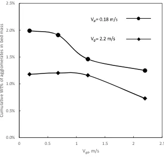
To understand the effect of gas velocity during injection on liquid distribution, Vgi is varied from 0.18 m/s to 2.2 m/s. In a Fluid CokerTM, the cross-sectional average superficial gas velocity varies from 0.24 m/s to approximately 0.9 m/s with the vertical position, and there are significant radial variations [5]: the range of gas velocity used in this study is, thus, set to include the range of velocities that could be expected in the spray region in the industrial case. Using the cold simulation experimental method, the amount and size distribution of agglomerates, and the initial liquid to solid ratio of agglomerates are obtained. The results in Figure 3.3 below show the cumulative weight percentage of agglomerates at different size cuts. When Vgi increases from 0.18 m/s to 1.2 m/s the total amount of agglomerates decreases while further increase of Vgi has minimal impact on the amount of agglomerates.

0 1 2 3 4 5 6 7

0 50 100 150

Volt

age

Time, s

(43)

28

Figure 0.3 Cumulative weight percentage of agglomerates in bed solid mass for various Vgi

while Vgd is constant at 0.18 m/s

0.0% 0.5% 1.0% 1.5% 2.0% 2.5%

100 1000 10000

Cum

Wt

%

o

f a

ggl

o

m

era

tes

in

b

ed

mas

s

(44)

29

Figure 0.4 The effect of Vgi on amount of macro and micro agglomerates while Vgd is

constant at 0.18 m/s

The results in figure 3.4 show that the increase of gas velocity during injection has no significant impact on the mass of micro agglomerates. The increase of gas velocity during injection from 0.18 m/s to 1.2 m/s contributed to the dropping of mass of macro agglomerates while at gas velocities higher than 1.2 m/s the mass of macro agglomerates remains at circa 0.37%. The total amount of agglomerates in the fluidized bed dropped drastically when gas velocity during injection changed from 0.18 m/s to 2.2 m/s. However, after the gas velocity reaches 1.2 m/s, the change in mass of agglomerates is minimal.

0.0% 0.5% 1.0% 1.5% 2.0% 2.5%

0.0 0.5 1.0 1.5 2.0 2.5

Wei gh t p erce n ta ge o f a ggl o m era tes in b ed solid mas s

Gas velocity during injection, m/s micro agglomerates

macro agglomerates

(45)

30

Figure 0.5 Cumulative fraction of water trapped in agglomerates various Vgi while Vgd is

constant at 0.18 m/s

The results in Figure 3.5 indicate the cumulative fraction of water trapped in agglomerates at different size cuts. When Vgi increases from 0.18 m/s to 1.2 m/s the total amount of agglomerates decreases while further increase of Vgi has minimal impact on the amount of agglomerates.

0% 10% 20% 30% 40% 50% 60% 70% 80% 90% 100%

100 1000 10000

Cumu

lat

iv

e

Fract

ion

o

f wat

er

tra

p

ed

(46)

31

Figure 0.6 Effect of Vgi on the total amount of free moisture

On one hand the fraction of free moisture in the total amount of liquid injected increases from 7.7% to 51.7% when gas velocity during injection rises from 0.18 m/s to 2.2 m/s. On the other hand, the quality of liquid to solid contact is hardly affected after the gas velocity reaches 1.2 m/s. It is suspected that a transition from bubbling regime to turbulent regime happened when the superficial gas velocity is at approximately 1.2 m/s. Tests of the pressure difference in the

fluidized bed need to be conducted to confirm the possible transition. 0

0.1 0.2 0.3 0.4 0.5 0.6

0 0.5 1 1.5 2 2.5

Fre

e

m

o

is

tu

re

/ wat

er

in

jec

ted

(47)

32

Figure 0.7 Initial L/S ratio in macro and micro agglomerates at various Vgi at constant

Vgd=0.18 m/s

Results in Figure 3.7 indicate that increasing the gas velocity during injection will slightly reduce the liquid to solid ratio in both macro and micro agglomerates while after Vgi reaches 1.2 m/s the impact is minimal. When the superficial gas velocity increases, in the region where solids and liquid interact, the liquid was more evenly distributed onto the particles. This is possibly because the at a higher superficial gas velocity, the ratio below the liquid and solids in the interaction region since more gas bubbles enter the interaction region which carry more solids in the wakes.

0 0.02 0.04 0.06 0.08 0.1 0.12 0.14 0.16

0 0.5 1 1.5 2 2.5

Liq u id to solid ra ito in a ggl o m era tes , L/S

Gas velocity during injection, m/s

Macro agglomerates

(48)

33

3.2.3 Effect of gas velocity during drying

Figure 0.8 Effect of increasing Vgd on the amount of agglomerates at different Vgi (0.18, 2.2

m/s)

Figure 3.8 shows that increasing gas velocity during drying is beneficial for liquid distribution when Vgi is either at 0.18 m/s or 2.2 m/s. A higher gas velocity during the drying stage

contributes to the breakup of agglomerates which releases the liquid that was trapped in agglomerates.

0% 10% 20% 30% 40% 50% 60% 70% 80% 90% 100%

0.0 0.5 1.0 1.5 2.0 2.5

Fre

e

m

ois

tu

re

/l

iqu

id

inj

ecte

d

, g/

g

(49)

34

Figure 0.9 Effect of Vgd on liquid to solid ratio when Vgi= 0.18 m/s and Vgi= 2.2 m/s

Figure 3.9 shows that increasing gas velocity during drying contributes to lower the liquid to solid ratio of the agglomerates when Vgi is either at 0.18 m/s or 2.2 m/s. A higher gas velocity during the drying stage contributes to the breakup of agglomerates which releases the liquid that was trapped in agglomerates.

0% 2% 4% 6% 8% 10% 12% 14% 16%

0.00 0.50 1.00 1.50 2.00 2.50

Liq

u

id

to

solid

ra

ito

in

a

ggl

o

m

era

tes

,

L/S

(50)

35

Figure 0.10 Effect of Vgd on amount of agglomerates when Vgi= 0.18 m/s and Vgi=2.2 m/s

The results in Figure 3.10 indicate that increasing gas velocity during drying contributes to a lower amount of agglomerates when Vgi is either at 0.18 m/s or 2.2 m/s. A higher gas velocity during the drying stage contributes to the breakup of agglomerates which makes the total amount of agglomerates lower.

0.0% 0.5% 1.0% 1.5% 2.0% 2.5%

0 0.5 1 1.5 2 2.5

Cumu

lat

iv

e

Wt

%

o

f a

ggl

o

m

era

tes

in

b

ed

mas

s

(51)

36

Effect of local gas velocity on the distribution of liquid in a fluidized

bed

In a Fluid CokerTM, superficial velocity increases as the height in the bed increases due to the steam from stripper section, attrition nozzles, feedstocks injected at different levels and the vapors produced by pyrolysis.

Previous studies have also found that a core-annulus structure exists in a fluid coker. In the annular region, the particles flow downwards and gas is carried down by the particles. In the core region gas rises rapidly and particles are carried upwards. The bed voidage increases gradually from the wall to the center of the bed without a sharp transition from the annular region and the core region. This means that in the core region the gas velocity is higher than superficial gas velocity at the same height. The location of feed nozzles in the bed determines the area which the sprays fall in.

The objective of this study is to better understand the effect on liquid distribution when the gas distribution changes at the same level as the jet. In comparison to the base case in which the initial gas distribution was even, gas velocity was increased in the region at the end of the jet or at the tip of the nozzle. Gum Arabic injections were conducted to characterize the liquid

distribution with various gas distributions.

4.1 Experimental setup and methodology

(52)

37

4.1.1 Initial gas distribution

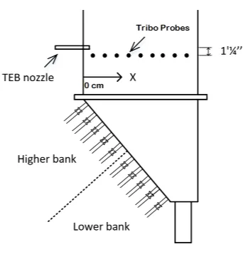
Figure 0.1 Schematic diagram of triboelectricity measurement system

The 20 sonic nozzles are defined into 2 banks. Each of the higher bank and the lower bank includes the 10 sonic nozzles. At a superficial gas velocity of 1 m/s, all the nozzles can provide the same gas velocity despite the different hydrostatic pressure in the bed.

(53)

38

For each experiment 10 gas sonic nozzles will be opened. Each open sonic nozzle contributes to 0.1 m/s of the total superficial velocity in the freeboard. The locations of open sonic nozzles are varied to create different initial gas distributions, for all of which the superficial velocity in the freeboard is maintained at 1 m/s.

4.1.2 Measurement of bubble gas flow in bed

A triboelectricity method has been successfully utilized by Portoghese et al.[17] to characterize the liquid–solid contacting efficiency by detecting the bed wetted area. Better liquid-solid contacting during injection leads to a more uniform distribution of liquid on bed particles which results in a larger bed wetted area. A larger bed wetted area produces a more intense electric current.

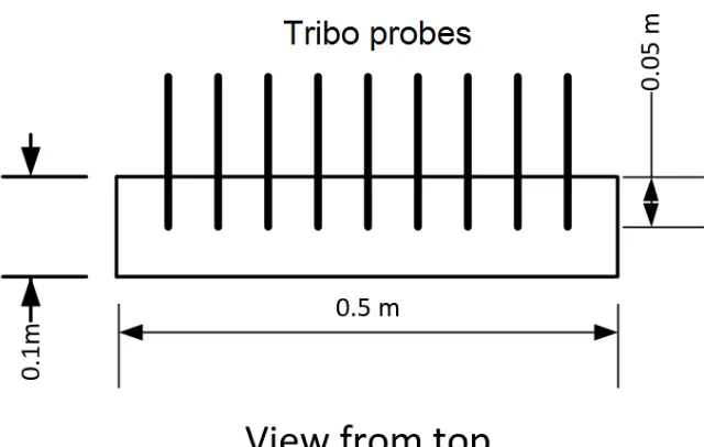
In this study, a triboelectricity method is used to detect the gas bubble flow in the fluidized bed. 9 triboprobes were installed horizontally on the bed wall as shown in Figure 4.3. The bed width is 50 cm and the distance between each probe is 5 cm. The distance that the probes penetrated into the bed is 5 cm.

(54)

39

Figure 0.3 Top view of locations of tribo probes

(55)

40

Figure 0.4 Raw signal of triboelectricity measurement, superficial gas velocity 1m/s

Figure 4.4 shows the raw signal of triboelectricity measurement. The frequency of the signal corresponds to the frequency of bubbles colliding with the tribo probe. The amplitude of the signal corresponds to the size of the bubble colliding with the tribo probe since larger bubbles carry more particles in the wakes.

Two parameters are derived from voltage signal over a frequency range of 0-100 Hz:

• Average Frequency (f)

• Power spectra density (P) -2

-1.5 -1 -0.5 0 0.5 1 1.5 2

0 2 4 6 8 10

Volt

age

(56)

41

Figure 0.5 Power spectra of triboelectricity measurement for a low bubble gas flowrate

Figure 0.6 Power spectra of triboelectricity measurement for a high bubble gas flowrate

Local volumetric flux of gas bubble is defined as

𝑞𝑏𝑖 = 𝛼𝑃𝑖 𝛽

𝑓_𝑖𝛾 4-1

α, β, γ are coefficients for the correlation. 0.00E+00 1.00E-06 2.00E-06 3.00E-06 4.00E-06 5.00E-06

0 20 40 60 80 100

Po w er sp ectra d en sity Frequency 0.00E+00 1.00E-06 2.00E-06 3.00E-06 4.00E-06 5.00E-06

0 20 40 60 80 100

(57)

42

Cross-sectional average volumetric flux can be derived as

𝑞_𝑏 ̅̅̅ = 1

∑λ𝑖[∑λ𝑖𝛼𝑃𝑖 𝛽

𝑓_𝑖𝛾] 4-2

We are interested in

𝑞𝑏𝑖 𝑞̅𝑏 =

𝑃_𝑖𝛽𝑓_𝑖𝛾 1

∑λ_𝑖[∑λ𝑖𝑃𝑖

𝛽

𝑓_𝑖𝛾] 4-3

α, β and γ are obtained by using data obtained at different superficial gas velocities, since for Group B powder:

𝑞𝑏

̅̅̅ = (V𝑔 – U𝑚𝑓) 4-4

4.2 Results and discussion

4.2.1 Radial profiles of bubble gas distribution

Triboelectricity signals acquired at 9 superficial velocities in the bed were used to obtain the coefficients in Equation 4.1. The best fit for coefficients α, β and γ is the values that produce a minimum value of

{(V𝑔 – U𝑚𝑓) − 1

∑λ_𝑖[∑λ𝑖𝛼𝑃𝑖 𝛽

𝑓_𝑖𝛾]} 2

Through calculation and fitting using the solver function in Excel, we can find that

𝑞_𝑏𝑖 = 5.168 × 10−5_𝑃

𝑖0.0949𝑓𝑖3.31 4-5

(58)

43

Figure 0.7 Correlation between the real average volumetric flux of bubble gas and the

average volumetric flux calculated

The correlation for gas-liquid jets from Benjelloun [28] was used to calculated the average jet penetration Ljet.

Three groups of gas distributions are measured. The base case is even distribution as shown below(a). Since it has 6 sonic nozzles open in the higher bank and 4 nozzles open in the lower bank, it is defined as 0.6-0.4 m/s. In the same way case b would be defined as 0.1-0.9 m/s and case c as 0.9-0.1 m/s.

y = 0.9942x + 0.0023 R² = 0.986

0.0 0.2 0.4 0.6 0.8 1.0 1.2

0 0.2 0.4 0.6 0.8 1 1.2

qb

fro

m

calcu

lat

ion

(59)

44

Figure 0.8 Group 1 gas distributions, (a) 0.6-0.4 m/s, (b) 0.1-0.9 m/s, (c) 0.9-0.1 m/s

0 0.5 1 1.5 2 2.5

0 10 20 30 40 50

qbi /qb

-a

ver

ag

e

lateral location, cm 0.9-0.1 m/s

0.1-0.9 m/s

Jet penetration 0.33 m

(60)

45

Figure 0.9 Profiles of gas bubble flow for Group 1 gas distributions. (The profile was

measured without the jet)

The tribo probes were placed 1.25 inch below the injection nozzle vertically. For the even gas distribution 0.6-0.4 m/s, the gas distribution is bed is not symmetrical due to the angled slope for gas distributors. The center of the profile, where the bubble gas flowrate is the highest, is closer to the left wall of the fluidized bed than to the right wall. For gas distribution 0.1-0.9 m/s, gas flowrate is higher at the end of the jet and the profile is almost flat. For gas distribution 0.9-0.1 m/s, gas flowrate is higher at the tip of the nozzle.

The second group of gas distributions are shown below.

(61)

46

Figure 0.11 Profiles of gas bubble flow for Group 2 gas distributions

The third group of gas distributions are shown below.

Figure 0.12 Group 3 gas distributions, (a) 0.6-0.4 m/s, (b) 0.3-0.7 m/s, (c) 0.7-0.3 m/s 0

0.5 1 1.5 2 2.5

0 10 20 30 40 50

qbi /qb

-a

ver

ag

e

lateral locatioin, cm 0.6-0.4 m/s 0.8-0.2 m/s

0.2-0.8 m/s

(62)

47

Figure 0.13 Profiles of gas bubble flow for Group 3 gas distributions 0

0.5 1 1.5 2 2.5

0 10 20 30 40 50

qbi /qb

-a

ver

ag

e

lateral location, cm 0.6-0.4 m/s

0.3-0.7 m/s 0.7-0.3 m/s

(63)

48

Figure 0.14 Summary of bubble gas flow radial profiles of various gas distributions

Because the gas distributors were located in an angled slope, the gas distribution in the fluidized bed was not symmetrical. Due to the hydrostatic pressure difference, the bubbles tend to shift to the left side of the bed (refer to figure 4.1). When the amount of gas initially put at the lower bank increases, bubble gas flowrate at the end of the jet increases gradually and an

approximately flat profile was achieved. When the amount of gas initially put at the higher bank increases, bubble gas flowrate at the tip of the nozzle increases gradually while a peak of the gas bubble flux exists close to the left wall.

0 0.5 1 1.5 2 2.5

0 10 20 30 40 50

qbi /qb

-a

ver

ag

e

lateral location, cm

0.1-0.9 m/s 0.2-0.8 m/s 0.3-0.7 m/s 0.7-0.3 m/s 0.8-0.2 m/s 0.9-0.1 m/s

(64)

49

4.2.2 Confirmation of gas distribution by entrainment tests

Figure 0.15 schematic diagram of the high gas velocity fluidized bed

(65)

50

Table 0-1 Mass of solids entrained in left and right internal cyclones at different gas

distributions

gas distribution

0.6-0.4 m/s 0.1-0.9 m/s 0.9-0.1 m/s

mass of sand entrained in left cyclone, g 800.5 1886 1809

mass of sand entrained in right cyclone, g 127 698 127

mass of sand entrained in left cyclone

mass of sand entrained in right cyclone 6.3 2.7 14.2

(66)

51

4.2.3 Effect of gas distribution on liquid distribution

Figure 0.16 Fraction of free moisture in mass of liquid injected (data for even distribution

is obtained from section 3.2.2)

The amount of free moisture increases drastically when the bubble gas flowrate becomes higher at the end of the jet. While increasing the bubble gas flowrate at the tip of the nozzle has no impact on the amount of free moisture. This result indicates that the agglomerates are majorly produced at the end of the jet.

0% 10% 20% 30% 40% 50% 60% 70% 80%

0 0.5 1 1.5 2 2.5

Fre

e

m

o

is

tu

re

/ in

jec

ted

liqu

id

Superficial velocity in freeboard during injection: Vgi, m/s 0.1-0.9 m/s

even distribution 0.3-0.7 m/s

(67)

52

Figure 0.17 weight percentage of agglomerates in bed mass

The amount of agglomerates decreases when the bubble gas flowrate becomes higher at the end of the jet. While increasing the bubble gas flowrate at the tip of the nozzle has no impact on the amount of agglomerates. This result also shows that the agglomerates majorly formed at the end of the jet.

0.0% 0.5% 1.0% 1.5% 2.0% 2.5%

0 0.5 1 1.5 2 2.5

Wt

%

o

f

agglome

ra

tes

in

b

ed

m

ass

Superficial velocity in freeboard during injection: Vgi, m/s

0.1-0.9 m/s

even distribution

0.9-0.1 m/s

(68)

53

Figure 0.18 liquid to solid ratio in agglomerates for gas distributions

The liquid to solid ratio in agglomerates decreases when the bubble gas flowrate becomes higher at the end of the jet. While increasing the bubble gas flowrate at the tip of the nozzle has a minimal impact on the liquid to solid ratio in agglomerates.

0.00 0.02 0.04 0.06 0.08 0.10 0.12 0.14 0.16 0.18 0.20

0 2000 4000 6000 8000 10000

Liq u id to solid ra tio in t h e a ggl o m era tes , L/S

Agglomerate size, micron

(69)

54

Effect of improvements in nozzle performance on the distribution

of liquid in a fluidized bed for various bed hydrodynamics

The effect of jet stability on liquid distribution has been studied by several researchers previously. A nozzle performance index (NPI) based on conductance measurements in the fluidized bed was used to characterize the liquid-solid contact during injection[20]. From various researches, the pulsations of jets were reported to have a beneficial impact on the liquid

distribution[21][22] on both small scale nozzles and industrial scale nozzles.

The effect of the atomization gas to liquid mass ratio (GLR) on liquid distribution has also been studied previously. NPIs based on different methods were utilized to characterize the liquid-solid contact[29][18]. Based on the geometry of nozzles, different impacts of GLR on the liquid distribution were reported.

In this study a high gas velocity fluidized bed with silica sand is used to investigate the effect of spray stability and gas to liquid ratio of injection (GLR). Pulsations in the spray are introduced by changing the geometry of the injection system. GLR is changed by changing the size of sonic nozzle for atomization gas and the upstream pressure by a regulator. The experiments performed to determine the impact of GLR were all conducted with stable sprays.

5.1 Experimental setup and methodology

(70)

55

Figure 0.1 Injection system for pulsating spray

(71)

56

In figure 5.1 and figure 5.2, the systems for stable spray and pulsating spray are displayed. Three parts are different. In the injection system for pulsating spray, the pre-mixer for atomization gas and liquid is Y connector with an internal diameter of 19 mm (3/4 inch). No restriction was put below the tank and the conduit leading to the nozzle tip has an internal diameter of 6.35 mm (1/4 inch). In the injection system for stable spray, the pre-mixer for atomization gas and liquid is T connector with an internal diameter of 6.35 mm (1/4 inch). A restriction that has a diameter of 1.016 mm was installed below the tank. The conduit leading to the nozzle tip has an internal diameter of 3.175 mm (1/8 inch).

Previous studies by Ariyapadi [27] have shown that the key factor that affects the stability of a spray is the flow pattern of gas and liquid in the conduit upstream of the nozzle tip. Figure 5.3 shows the flow pattern map for gas-liquid flow in a horizontal conduit.

Figure 0.3 Flow pattern map of Taitel and Dukler [30]. The dotted line refers to the modified transition line between the intermittent and annular regimes, as proposed by

Barnea et al [31]. Stable spray

(72)

57

Table 0-1 Linear velocities of liquid and atomization gas in different sizes of conduits

Conduit diameter 1/4 inch (unstable spray)

Inner diameter of conduit, m 0.00635 Inner diameter of conduit, m 0.00635

Area, m2 _0.000032 _{Area, m}2 _0.000032

Volume flowrate m3/s 0.000024 Volume flowrate m3/s 0.00003

ULS, m/s 0.76 UGS, m/s 0.94

Conduit diameter 1/8 inch (stable spray)

Inner diameter of conduit, m 0.003175 Inner diameter of conduit, m 0.003175

Area, m2 _{0.0000079 Area, m}2 _0.000079

Volume flowrate m3/s 0.000024 Volume flowrate m3/s 0.00003

ULS, m/s 3.03 UGS, m/s 3.77

The gas and liquid superficial velocities in the injection system for a stable spray is higher than in the system for a pulsating spray. When the UGS and ULS combination falls in the region of dispersed bubble, the flow has a tendency to be more stable. Open air injection shows that when the gas and liquid superficial velocity is in the disperse bubble region, the injection is improved by producing fewer pulsations. A regular video camera with a frequency of 1 frame every 30 ms is used to record the open air injection process. The pictures below show the expansion of the liquid jet during different times of injection. A more sophisticated analysis, developed in Chapter 2 (section 2.4), was used to characterize the spray stability.

(73)

58

c. t= 0.57 s d. t= 0.60 s

Figure 0.4 Pictures of spray (pulsating spray, t=0 is the beginning of injection)

5.1.2 Gas to liquid ratio (GLR)

In previous chapters, GLR was set at 2% for all injection experiments. In this study, GLR will be changed from 1% to 3.5%. The injection system used was the same as shown in Figure 5.2, which creates a relatively stable spray. First open air spray experiments were performed to verify the stability of the sprays. The Gum Arabic injection experiments were conducted subsequently to investigate the effect of different GLRs on the liquid-solid contact. The liquid flowrate was the same for all experiments and the gas-liquid flow through the spray nozzle throat was always in the sonic regime. Vgi and Vgd are kept constant at 0.68 m/s for all of these experiments.

5.1.3 Jet expansion angle

(74)

59

5.2 Results and discussion

5.2.1 Spray stability

η⁄η ̅ can effectively characterize the stability of different sprays. For a perfectly stable spray

η⁄η ̅ should be equal to 1 constantly. In this way there is no need to calibrate for αs.

Figure 0.5 Stability analysis for pulsating spray, GLR=2.2%, FL=21.4 g/s

0 0.5 1 1.5 2 2.5 3 3.5 4

0 1 2 3 4 5 6 7 8

η⁄η ̅

(75)

60

Figure 0.6 Stability analysis for stable spray GLR=2.2%, FL=21.4 g/s

The frequency of pulsations in the pulsating spray is approximately 5 Hz. The magnitude of the fluctuations in the spray area is significantly higher than for the stable spray. At the beginning of the stable spray, a pulse is detected and afterwards the spray tends to stabilize at around η⁄η ̅ =1.

5.2.2 Effect of spray stability on liquid distribution

Below shows the difference in free moisture, agglomerate mass and L/S of agglomerates for stable and unstable sprays at various gas velocities.

0 0.5 1 1.5 2 2.5 3 3.5 4

0 1 2 3 4 5 6 7 8

η⁄η ̅

(76)

61

Figure 0.7 Cumulative Wt% of agglomerates in bed mass GLR=2.2%, FL=21.4 g/s (two

experiments for each condition) 0.0%

0.5% 1.0% 1.5% 2.0% 2.5%

100 1000 10000

Cum

Wt

%

o

f a

ggl

o

m

era

tes

Size cut, µm

________{: stable spray} ---: pulsating spray

Vgi= 0.18 m/s

(77)

62

Figure 0.8 Initial L/S ratio in agglomerates (g/g) GLR=2.2%, FL=21.4 g/s

Figure 0.9 Cumulative fraction of water trapped in agglomerates GLR=2.2%, FL=21.4 g/s

0% 5% 10% 15% 20% 25%

0 2000 4000 6000 8000 10000

Liq u id to solid ra tio o f agglome ra tes , L/S

Size cut, μm

Vgi= 0.18 m/s

Vgd= 0.18 m/s

0% 10% 20% 30% 40% 50% 60% 70% 80% 90% 100%

100 1000 10000

Fract ion o f wat er tra p p ed

Size cut, μm

Vgi= 0.18 m/s

(78)

63

When the fluidization velocity during injection, Vgi, was 0.18 m/s and when the fluidization velocity during drying, Vgd, was 0.18 m/s, spray pulsation has a minimal impact on the free moisture and the liquid to solid ratio. Thus the free moisture is not affected in any significant manner. When the superficial velocity is low in both liquid injection stage and agglomerate drying stage, bed hydrodynamics is the dominant factor determining the liquid distribution.

Figure 0.10 Cumulative Wt% of agglomerates in bed mass GLR=2.2%, FL=21.4 g/s

0.0% 0.5% 1.0% 1.5% 2.0% 2.5%

100 1000 10000

C

u

m

Wt%

o

f a

gg

lom

erates

Size cut, µm

Vgi= 0.18 m/s

(79)

64

Figure 0.11 Initial L/S ratio in agglomerates (g/g) GLR=2.2%, FL=21.4 g/s

Figure 0.12 Cumulative fraction of water trapped in agglomerates GLR=2.2%, FL=21.4 g/s

0% 5% 10% 15% 20% 25%

0 2000 4000 6000 8000 10000

Liq u id to solid ra tio o f agglome ra tes , L/S

Size cut, µm

Vgi= 0.18 m/s

Vgd= 0.68 m/s

0% 10% 20% 30% 40% 50% 60% 70% 80% 90% 100%

100 1000 10000

Fract ion o f wat er tra p p ed

Size cut, μm

Vgi= 0.18 m/s

Effect of Local Bed Hydrodynamics on the Distribution of Liquid in a Fluidized Bed

Scholarship@Western

Scholarship@Western

Effect of Local Bed Hydrodynamics on the Distribution of Liquid in

Effect of Local Bed Hydrodynamics on the Distribution of Liquid in

a Fluidized Bed

a Fluidized Bed

Abstract

Acknowledgement

Table of contents

List of tables

List of figures

Lists of symbols

Introduction

1.1 Fluid Coking

1.2 Bed hydrodynamics

1.3 Liquid distribution and agglomeration

1.4 Spray performance

1.4.1 Atomization gas to liquid ratio (GLR)

1.4.2 Spray stability

1.5 Thesis Objectives

Experimental setup and methodology

2.1 Equipment and material

2.2 Bed conductance measurements

2.3 Cold simulation experimental model

2.3.1 Agglomerate size distribution

2.3.2 Initial liquid to solid ratio

2.4 Jet stability measurement

Single pixel

2.5 Jet expansion angle

Effect of high gas velocity on the distribution of liquid in a fluidized

bed

3.1 Experimental setup and methodology

3.2 Results and discussion

3.2.1 Preliminary tests

3.2.2 Effect of gas velocity during injection

3.2.3 Effect of gas velocity during drying

Effect of local gas velocity on the distribution of liquid in a fluidized

bed

4.1 Experimental setup and methodology

4.1.1 Initial gas distribution

4.1.2 Measurement of bubble gas flow in bed

4.2 Results and discussion

4.2.1 Radial profiles of bubble gas distribution

4.2.2 Confirmation of gas distribution by entrainment tests

4.2.3 Effect of gas distribution on liquid distribution

Effect of improvements in nozzle performance on the distribution

of liquid in a fluidized bed for various bed hydrodynamics

5.1 Experimental setup and methodology

5.1.2 Gas to liquid ratio (GLR)

5.1.3 Jet expansion angle

5.2 Results and discussion

5.2.1 Spray stability

5.2.2 Effect of spray stability on liquid distribution