Visualization of Eddy Current Distributions for Arbitrarily Shaped
Coils Parallel to a Moving Conductor Slab
Toshiya Itaya1, *, Koichi Ishida2, Yasuo Kubota3, Akio Tanaka4, and Nobuo Takehira2
Abstract—To visualize eddy current distribution (ECD) of an arbitrarily shaped coil arranged parallel to a moving conductor slab, an exact theoretical solution is derived using an analytical method based on the double Fourier transform method. The arbitrarily shaped coil is regarded as a plane coil of a single turn, and both DC and AC excitation currents can be applied. Furthermore, ECD charts are obtained when the conductor slab is moving. We calculate some examples with respect to a circular coil, rectangular coil, and triangular coil and show the effect of coil excitation frequency and speed of the conductor on ECDs. Results show that the eddy current generated in the moving conductor slab is composed of current induced by the excitation frequency and conductor speed.
1. INTRODUCTION
Eddy current applications have produced various industry technologies, e.g., eddy current testing,
induction heating and eddy current sensors. Eddy current testing is used to detect defects in
structural materials such as steel, aluminum, titanium and carbon-fiber-reinforced plastic [1]. Induction heating is used in commercial cooking and heat treatment. Eddy current sensors are widely used for displacement [2], conductivity [3] and thickness measurements [4]. These measurements use the change in eddy currents magnitude to measure the physical quantity of interest. However, because the eddy current cannot be measured directly, it is difficult to determine the eddy current distribution (ECD). Furthermore, when a conductor is moved, the behavior of the eddy current becomes complicated. Therefore, theoretical analysis to clarify the ECD is strongly desired. The behavior of an eddy current strongly depends on factors such as coil shape, excitation frequency, conductor speed and conductor
properties [5]. These complex dependencies have thus far prevented the development of a precise
theoretical analysis of ECD.
Dodd and Deeds presented an analytical solution for the eddy current density induced by the circular coil arranged parallel to a conductor slab using the integral of the Bessel function [6]. Thus, the basic phenomenon of the relationship between eddy current density and skin depth has been described. Panas and Papayiannakis represented the magnetic vector potential by a filamentous elliptical coil in a Cartesian coordinate system; the solution of partial differential equations is obtained in the form of a 2D Fourier transform, which then allows the inverse Fourier transform of the magnetic flux density and eddy current density to be calculated [7]. Analytical expressions are also given for the ECD of a circular coil arranged perpendicular [8] or tilted [9] to the conductor slab. Theodoulidis and Kriezis obtained an analytical solution for ECD of a rectangular coil by introducing a concept called secondary vector potential [10]. When ECD is considered for conductors in motion, the skin effect due to velocity
Received 12 January 2016, Accepted 24 February 2016, Scheduled 15 March 2016
* Corresponding author: Toshiya Itaya ([email protected]).
1 Department of Electronic and Information Engineering, National Institute of Technology, Suzuka College, Suzuka 510-0294, Japan.
2 Department of Mechanical and Electrical Engineering, National Institute of Technology, Tokuyama College, Shunan 745-8585,
Japan. 3 Kohan Kogyo Co., Ltd., Kudamatu 744-0011, Japan. 4 Department of Electrical Engineering, National Institute of
is affected is known. When a DC excitation coil is moved, using the second vector potential in place of the magnetic vector potential, the analytical solution can be shown in Fourier space by a 2D Fourier transform [11]. Panas and Kriezis represented an analytical solution for the case when the DC excitation filamentary rectangular coil is moved by a 3D Fourier transform with respect to time and space; these results are numerically computed by a fast Fourier algorithm from the inverse Fourier transform [12]. When both the AC excitation coil and conductor slab are moved, the eddy current generated by them should be considered. An analytical method have been already proposed based on the double Fourier transform method that considers the case of the conductor slab moving in relation to the rectangular coil [13].
In the present study, a new technique to visualize the ECD in a conductor slab due to an arbitrarily shaped coil is proposed. The arbitrarily shaped coil is regarded as a plane coil of a single turn, and both DC and AC excitation current can be applied. Furthermore, ECD charts were visualized when the conductor slab is moving. Some examples with respect to a circular coil, rectangular coil and triangular coil were calculated and the effect of coil excitation frequency and the speed of the conductor on visualized ECDs were shown.
2. THEORETICAL ANALYSIS
Figure 1 shows the geometry of the analytical model. The surface of the conductor is matched to the
z = 0 plane. The distance between the coil and slab is z0. To facilitate magnetic field analysis, the
following assumptions are made. The moving conductor is isotropic and infinitely wide. The coil is
a one-turn coil and carries current I with a known effective rms value and angular frequency ω. The
coil wire is assumed to be infinitely thin. The conductivity σ, permeability μ and conductor speed
¯
v = (vx, vy,0) are constant. In the quasi-steady state, the displacement current is negligible and the
following equations are obtained:
∇ ×H¯ = ¯J (1)
∇ ×E¯ = −∂B¯
∂t (2)
∇ ·B¯ = 0 (3)
where
∇ ·J¯= 0 (4)
Since conductor speed ¯v = (vx, vy,0) is very small in comparison with light velocity, the next
x
y
0
z
d
vx
σ,μ vy
v I
z0
equations are obtained:
¯
J = σ( ¯E+ ¯v×B¯) (5)
¯
B = μH¯ (6)
To solve Maxwell’s equation, a double Fourier transform and its inverse are introduced as follows
b(ξ, η, z) =
∞
−∞
∞
−∞B(x, y, z)e
j(xξ+yη)
dxdy (7)
B(x, y, z) = 1 4π2
∞
−∞
∞
−∞b(ξ, η, z)e
−j(xξ+yη)
dξdη (8)
2.1. Magnetic Flux Densities Produced by an Arbitrarily Shaped Planar Coil
According to Appendix A, thex-,y- andz-components of the magnetic flux density ¯B in the conductor
slab are given by
Bx = μ80μrI
π2
∞
−∞
∞
−∞
ξ η(1−e2γd)
−(1 +λ0)e2γd+ν0
×e
γ−√ξ2+η2
d
eγz+
1 +λ0−ν0e
γ−√ξ2+η2
d
e−γz
×e−z0√ξ2+η2S(ξ, η)e−j(xξ+yη)dξdη (9)
By = μ80μrI
π2
∞
−∞
∞
−∞
1 1−e2γd
−(1 +λ0)e2γd+ν0
×e
γ−√ξ2+η2d
eγz+
1 +λ0−ν0e
γ−√ξ2+η2d
e−γz
×e−z0
√
ξ2+η2S(ξ, η)e−j(xξ+yη)
dξdη (10)
Bz = jμ
0μrI
8π2
∞
−∞
∞
−∞
ξ2+η2 ηγ(1−e2γd)
−(1 +λ0)e2γd+ν0
×e
γ−√ξ2+η2d
eγz−
1 +λ0−ν0e
γ−√ξ2+η2d
e−γz
×e−z0√ξ2+η2S(ξ, η)e−j(xξ+yη)
dξdη (11)
Here,S(ξ, η) is called the shape function [14] and defined as
S(ξ, η) =
n
i=1
xi
xi−1
ej{xξ+fi(x)η}dx (12)
whereμr =μ/μ0 and
γ =
ξ2+η2−jσμ
0μr(vxξ+vyη) +jωσμ0μr (13)
λ0 =
γ2−μr2
ξ2+η2 1−e−2γd
γ+μr
ξ2+η22−γ−μ r
ξ2+η22e−2γd
(14)
ν0 =
4μrγ
ξ2+η2e(√ξ2+η2−γ)d
(γ+μr
ξ2+η2)2−(γ−μ r
ξ2+η2)2e−2γd (15)
Quantitiesξandηare integration variables of the Fourier transform; furthermore,λ0andν0depend
2.2. Eddy Current Densities Produced by an Arbitrarily Shaped Planar Coil
The x- andy-components of eddy current density ¯J produced in the conductor slab by the arbitrarily
shaped planar coil can be described as
Jx =
1
μ0μr
∂Bz
∂y − ∂By
∂z
(16)
Jy =
1
μ0μr
∂Bx
∂z − ∂Bz
∂x
(17)
which can be solved as follows
Jx = −8I
π2
∞
−∞
∞
−∞
γ2−ξ2−η2 γ(1−e2γd)
−(1 +λ0)e2γd+ν0
× e
γ−√ξ2+η2
d
eγz−
1 +λ0−ν0e
γ−√ξ2+η2
d
e−γz
×e−z0√ξ2+η2S(ξ, η)e−j(xξ+yη)dξdη (18)
Jy = 8Iπ2
∞
−∞
∞
−∞
ξγ2−ξ2−η2 ηγ(1−e2γd)
−(1 +λ0)e2γd+ν0
× e
γ−√ξ2+η2d
eγz−
1 +λ0−ν0e
γ−√ξ2+η2d
e−γz
×e−z0√ξ2+η2S(ξ, η)e−j(xξ+yη)dξdη (19)
2.3. Stream Function
The eddy current density obtained above in conjunction with the stream function is used to visualize
ECD. The eddy current streamline in thexy plane is described by
dy dx =
Re (Jy)
Re (Jx)
(20)
Therefore, we have
Re (Jy)dx−Re (Jx)dy = 0 (21)
where operator Re( ) returns the real part of the arguments and provides the instantaneous value of eddy current density. Stream functionU(x, y) in thexy plane is given by
U(x, y, z) = Re
Jydx
=k = constant (22)
or
U(x, y, z) = Re
−Jxdy
=k = constant (23)
Equation (21) may be used in either Equation (22) or (23). This paper uses Equation (22) in
Equation (21). Since the eddy current in a conductor slab changes over time, it is a function of timet.
Therefore, stream function U(x, y, z, t) is given by
U(x, y, z, t) = Re
Jydx
√
2ejωt
=√2
Re
Jydx
cosωt−Im
Jydx
sinωt
=k (24)
where operator Im( ) returns the imaginary part of the arguments and provides the instantaneous value of eddy current density. In the above equations, constantkis obtained by substituting point (x, y) with
eddy current at timetonzplane is obtained. In addition, the integral in Equation (24) may be written as
Jydx = j8I
π2
∞
−∞
∞
−∞
−jσμ0μr(vxξ+vyη) +jωσμ0μr
η
×T e−z0√ξ2+η2S(ξ, η)e−j(xξ+yη)
dξdη (25)
T = 1
γ(1−e2γd)
−(1 +λ0)e2γd+ν0e
γ−√ξ2+η2d
eγz
−
1 +λ0−ν0e
γ−√ξ2+η2
d
e−γz (26)
2.4. Shape Function
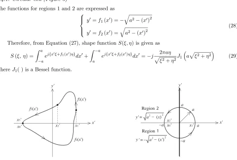
The shape function depends on the coil shape. When the coil is divided into three pieces of closed curve, each closed curve carries the same current, as shown in Figure 2. If they are described as y =f1(x),
f2(x) and f3(x), the shape function is obtained as follows by integrating counter clockwise
S(ξ, η) =
x1
x0
ej{xξ+f1(x)η}dx+
x2
x1
ej{xξ+f2(x)η}dx+
x3
x2
ej{xξ+f3(x)η}dx (27)
Next, the shape functions for a circular coil, rectangular coil and triangular coil using Equation (27) are derived. The center of the coils is the centroid of the shape.
2.4.1. Circular coil (Figure 3)
The functions for regions 1 and 2 are expressed as
⎧ ⎪ ⎨ ⎪ ⎩
y =f1(x) =−
a2−(x)2
y =f2(x) =
a2−(x)2
(28)
Therefore, from Equation (27), shape functionS(ξ, η) is given as
S(ξ, η) =
a
−a
ej{xξ+f1(x)η}dx+
−a
a
ej{xξ+f2(x)η}dx =−j2πaη
ξ2+η2J1
aξ2+η2 (29)
whereJ1( ) is a Bessel function.
y'
x'
x1'
x0' x2'
f1(x')
f2(x')
f3(x')
x3'
Figure 2. Arbitrarily shaped planar coil which is divided into three pieces of closed curve.
y'
x' a
−a
a
−a
a
Region2
Region1
x1'
x0'
x2'
2 2−
y a (x')
2 2−
y'= a (x)
'=−
2.4.2. Rectangular coil (Figure 4)
The functions for regions 1 and 2 are expressed as
y =f1(x) =−b
y =f2(x) =b (30)
Therefore, from Equation (27), shape functionS(ξ, η) is given as
S(ξ, η) =
a
−a
ej{xξ+f1(x)η}dx+
−a
a
ej{xξ+f2(x)η}dx =−j4
ξsin (aξ) sin (bη) (31)
2.4.3. Triangular coil (Figure 5)
The functions for lines 1, 2 and 3 are expressed as follows:
⎧ ⎪ ⎪ ⎪ ⎪ ⎨ ⎪ ⎪ ⎪ ⎪ ⎩
y =f1(x) =−b
3
y =f2(x) =−b
ax
+ 2
3b
y =f3(x) = b
ax
+2
3b
(32)
Therefore, from Equation (27), shape functionS(ξ, η) is given as
S(ξ, η) =
a
−a
ej{xξ+f1(x)η}dx+
0
a
ej{xξ+f2(x)η}dx+
−a
0
ej{xξ+f3(x)η}dx
= e−jb3η
2
ξsin (aξ) +
2a
a2ξ2−b2η2 {bηsin (bη)−aξsin (aξ)}
+j 2abη
a2ξ2−b2η2 {cos (aξ)−cos (bη)} (33)
y'
x' b
−a a
Region 2
y'=b
Region 1
y'=−b
x1'
x0'
x2'
−b
Figure 4. Rectangular coil with length 2a and width 2b.
y'
x'
−a a
Line1
x1'
x0'
x2'
Line2
Line3
2 3 b
y' = x' b
a
3 b y'
2 3 b
y' = x' b
a
2 3b
3 b
+ − +
=−
Figure 5. Triangular coil with base length 2a
and height b.
3. RESULTS AND DISCUSSION
From Equation (24), the visualized ECD as a function of excitation frequency and conductor speed are
obtained. The y (x)-direction corresponds to the horizontal (vertical) axis. ECD is given for z = 0
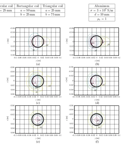
Table 1. Specifications of coils.
Circular coil Rectangular coil Triangular coil
a= 25 mm a= 50 mm a= 25 mm
b= 25 mm b= 75 mm
Table 2. Specifications of conducting slab.
Aluminum
σ= 3×10⁷S/m
d= 10 mm
μr= 1
-0.06
-0.04
-0.02
0
0.02
0.04
0.06
x
[m]
-0.1 -0.08 -0.06 -0.04 -0.02 0 0.02 0.04 0.06 0.08 0.1
y [m]
-0.06
-0.04
-0.02
0
0.02
0.04
0.06
x
[m]
-0.1 -0.08 -0.06 -0.04 -0.02 0 0.02 0.04 0.06 0.08 0.1
y [m]
-0.06
-0.04
-0.02
0
0.02
0.04
0.06
x
[m]
-0.1 -0.08 -0.06 -0.04 -0.02 0 0.02 0.04 0.06 0.08 0.1
y [m]
-0.06
-0.04
-0.02
0
0.02
0.04
0.06
x
[m]
-0.1 -0.08 -0.06 -0.04 -0.02 0 0.02 0.04 0.06 0.08 0.1
y [m]
-0.06
-0.04
-0.02
0
0.02
0.04
0.06
x
[m]
-0.1 -0.08 -0.06 -0.04 -0.02 0 0.02 0.04 0.06 0.08 0.1
y [m]
-0.06
-0.04
-0.02
0
0.02
0.04
0.06
x
[m]
-0.1 -0.08 -0.06 -0.04 -0.02 0 0.02 0.04 0.06 0.08 0.1
y [m]
(a) (b)
(c) (d)
(e) (f)
-20
20 60
60
20
-20 -60 100
70 50 30
10
10 -20
20 60 100
250
150 50
250
150
50
Figure 6. ECDs for a circular coil when excitation frequency and conductor speed change. (a) DC,
v = 10 m/s, (b) DC, v = 20 m/s, (c) f = 100 Hz, v = 10 m/s, (d) f = 100 Hz, v = 20 m/s, (e)
f = 1000 Hz, v= 10 m/s and (f)f = 1000 Hz, v= 20 m/s.
current. The thick line represents the coil line (i.e., Figures 6–8). The distance between the coil and
the conducting slab is z0 = 10 mm. The coil was excited by a 1 A current. The excitation frequency
was set to 0 (DC), 100 and 1000 Hz. Table 1 shows the specifications of the coils and Table 2 shows
the specifications of the conducting slab. The conductor speed was set tovy =v= 10 and 20 m/s. The
conductor slab was allowed to move only in the y-direction (vx = 0). A positive value represents the
a negative value represents the magnitude of the eddy currents in the same direction relative to the direction of the coil current.
Figure 6 shows ECD for a circular coil. At DC and v = 10 m/s or 20 m/s, two current vortexes
with different polarities were generated in the y-direction. Atf = 100 Hz andv = 10 m/s, two current
vortexes with similar polarities were generated in they-direction. Atv= 20 m/s, their polarities became
opposite. At v = 20 m/s, their polarities became opposite. At f = 1000 Hz, only a single vortex was
generated. At this frequency, the size of the eddy current increased, but the speed did not affect the ECD.
Figure 7 shows ECD for a rectangular coil. At DC andv= 10 m/s or 20 m/s, two current vortexes
with different polarities were generated in the y-direction. Atf = 100 Hz andv = 10 m/s, two current
vortexes with similar polarities were generated in they-direction. Atv= 20 m/s, their polarities became
opposite. At f = 1000 Hz, only a single vortex was generated. At this frequency, the size of the eddy
current increased, but the speed did not affect the ECD. The single vortex had a smooth shape with rounded corners of the coil.
-0.06
-0.04
-0.02
0
0.02
0.04
0.06
x
[m]
-0.1 -0.08 -0.06 -0.04 -0.02 0 0.02 0.04 0.06 0.08 0.1
y [m]
(a)
-0.06
-0.04
-0.02
0
0.02
0.04
0.06
x
[m]
-0.1 -0.08 -0.06 -0.04 -0.02 0 0.02 0.04 0.06 0.08 0.1
y [m]
(b)
-0.06
-0.04
-0.02
0
0.02
0.04
0.06
-0.1 -0.08 -0.06 -0.04 -0.02 0 0.02 0.04 0.06 0.08 0.1
y [m]
(c)
-0.06
-0.04
-0.02
0
0.02
0.04
0.06
-0.1 -0.08 -0.06 -0.04 -0.02 0 0.02 0.04 0.06 0.08 0.1
y [m]
(d)
-0.06
-0.04
-0.02
0
0.02
0.04
0.06
-0.1 -0.08 -0.06 -0.04 -0.02 0 0.02 0.04 0.06 0.08 0.1
y [m]
(e)
-0.06
-0.04
-0.02
0
0.02
0.04
0.06
-0.1 -0.08 -0.06 -0.04 -0.02 0 0.02 0.04 0.06 0.08 0.1
y [m]
(f)
x
[m]
x
[m]
x
[m]
x
[m]
20
20 20
60
-20
20 20
-60
-60 -20
60 100
20 100 20
20
60
20 20
-20 100
60
300
200
300
200 100 100
Figure 7. ECDs for a rectangular coil when excitation frequency and conductor speed change. (a)
DC, v = 10 m/s, (b) DC, v = 20 m/s, (c) f = 100 Hz, v = 10 m/s, (d) f = 100 Hz, v = 20 m/s, (e)
-0.06
-0.04
-0.02
0
0.02
0.04
0.06
x
[m]
-0.1 -0.08 -0.06 -0.04 -0.02 0 0.02 0.04 0.06 0.08 0.1 y [m]
(a)
-0.06
-0.04
-0.02
0
0.02
0.04
0.06
x
[m]
-0.1 -0.08 -0.06 -0.04 -0.02 0 0.02 0.04 0.06 0.08 0.1 y [m]
(b)
-0.06
-0.04
-0.02
0
0.02
0.04
0.06
x
[m]
-0.1 -0.08 -0.06 -0.04 -0.02 0 0.02 0.04 0.06 0.08 0.1 y [m]
(c)
-0.06
-0.04
-0.02
0
0.02
0.04
0.06
x
[m]
-0.1 -0.08 -0.06 -0.04 -0.02 0 0.02 0.04 0.06 0.08 0.1 y [m]
(d)
-0.06
-0.04
-0.02
0
0.02
0.04
0.06
x
[m]
-0.1 -0.08 -0.06 -0.04 -0.02 0 0.02 0.04 0.06 0.08 0.1 y [m]
(e)
-0.06
-0.04
-0.02
0
0.02
0.04
0.06
x
[m]
-0.1 -0.08 -0.06 -0.04 -0.02 0 0.02 0.04 0.06 0.08 0.1 y [m]
(f)
-20 60
20
100 60
20
-20
70 50
30
10
100 60
20
-20
150 50
150 50
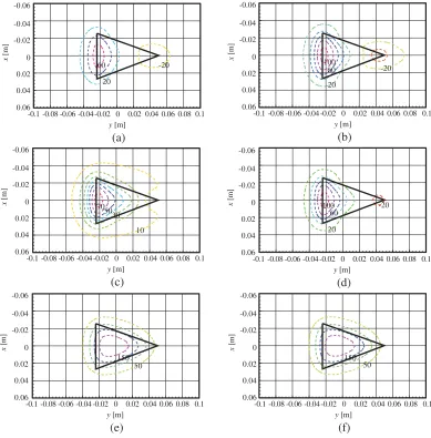
Figure 8. ECDs for a triangular coil when excitation frequency and conductor speed change. (a)
DC, v = 10 m/s, (b) DC, v = 20 m/s, (c) f = 100 Hz, v = 10 m/s, (d) f = 100 Hz, v = 20 m/s, (e)
f = 1000 Hz, v= 10 m/s and (f)f = 1000 Hz, v= 20 m/s.
Figure 8 shows ECD for a triangular coil. At DC andv = 10 m/s or 20 m/s, two current vortexes
with different polarities were generated in the y-direction. Atf = 100 Hz and v= 10 m/s, the current
vortex was greatly distorted in the y-direction. At v = 20 m/s, two current vortexes with opposite
polarities were generated in the y-direction. At f = 1000 Hz, the size of the eddy current increased,
but the speed did not affect the ECD. At this frequency, only a single vortex was generated and had a smooth shape with rounded corners of the coil.
Consequently, it is considered that the eddy current generated in the moving conductor slab is composed of current induced by the excitation frequency and conductor speed. When the eddy current
generated by the conductor speed is dominant (e.g., at f = 100 Hz and 20 m/s), one current vortex
is produced in the region of the conductor slab close to the coil. It is generated in the direction that reduces magnetic flux from the coil. The other current vortex is produced in the region of the conductor slab away from the coil, and it is generated in the direction that increases magnetic flux from the coil. Similar results were obtained with the DC excitation current. When the eddy current generated by the
excitation frequency is dominant (e.g., at f = 1000 Hz and 10 m/s or 20 m/s), the impact of moving
4. CONCLUSION
In this study, we derive an exact theoretical solution that visualizes ECD for an arbitrarily shaped coil arranged parallel to a conductor slab, a problem that heretofore remains unsolved. We determine that the eddy current flow in the conductor depends on the excitation frequency and speed of the conductor slab relative to the coil. The visualized ECD in the conductor, which is necessary to advance eddy current testing, induction heating and eddy current sensing, can be obtained from this new analysis.
APPENDIX A.
From Equations (1)–(3), (5) and (6), the magnetic density ¯B in the moving conductor slab (this region
is defined by −d < z <0 and coincides with the conductor itself) is obtained as follows [13]
∇2¯
B−σμvx∂
¯
B
∂x −σμvy ∂B¯
∂y −jωσμB¯ = ¯0 (A1)
Using Equation (7), Fourier transform of Equation (A1) gives
∂2¯b
∂z2 −
ξ2+η2−jσμvxξ−jσμvyη+jωσμ
¯
b= ¯0 (A2)
Solving the above equation, the x-, y- and z-components of the magnetic flux density ¯b in the
conductor slab are given by [13]
bx = Cxeγz+Dxe−γz (A3)
by = Cyeγz+Dye−γz (A4)
bz = Czeγz+Dze−γz (A5)
where
γ=
ξ2+η2−jσμ(v
xξ+vyη) +jωσμ (A6)
The coefficientsCx,Cy,Cz,Dx,Dy and Dz in Equations (A3)–(A5) are obtained as follows [13]
Cx = 1−μr
e2γd
−(1 +λ0)e2γd+ν0e
γ−√ξ2+η2d
Cix (A7)
Cy = 1−μr
e2γd
−(1 +λ0)e2γd+ν0e
γ−√ξ2+η2d
Ciy (A8)
Cz = 1−μer2γd
−(1 +λ0)e2γd+ν0e
γ−√ξ2+η2
d ξ2+η2
γ Ciz (A9)
Dx = 1−μer2γd
1 +λ0−ν0e
γ−√ξ2+η2d
Cix (A10)
Dy = 1−μr
e2γd
1 +λ0−ν0e
γ−√ξ2+η2d
Ciy (A11)
Dz = −1−μr
e2γd
1 +λ0−ν0e
γ−√ξ2+η2d ξ2+η2
γ Ciz (A12)
where μr = μ/μ0. The coefficients Cix, Ciy and Ciz are determined by the coil geometry.
Equations (A7)–(A12) are determined from boundary conditions.
As shown in Figure 1, when an arbitrarily shaped coil, which is positioned atz=z0 and carrying
current I, the x-, y- and z-components of magnetic flux density ¯bi(ξ, η, z) at z < z0 are described as
follows [14]
bix = μ20Iξ
η e
(z−z0)√ξ2+η2
n
i=1
xi
xi−1
ej{xξ+fi(x)η}dx=C
ixez
√
biy = μ20Ie(z−z0)
√
ξ2+η2
n
i=1
xi
xi−1
ej{xξ+fi(x)η}dx=C
iyez
√
ξ2+η2 (A14)
biz = jμ0I
ξ2+η2
2η e
(z−z0)√ξ2η+η2
n
i=1
xi
xi−1
ej{xξ+fi(x)η}dx=C
izez
√
ξ2+η2 (A15)
Therefore, using shape functionS(ξ, η) yields
Cix = μ20ηIξe−z0
√
ξ2+η2S(ξ, η) (A16)
Ciy = μ20Ie−z0
√
ξ2+η2S(ξ, η) (A17)
Ciz = jμ0I
ξ2+η2
2η e
−z0√ξ2+η2S(ξ, η) (A18)
From Equations (A3)–(A5) and (A7)–(A12), thex-,y- and z-components of magnetic flux density
¯b(ξ,η,z) at the moving conductor slab are described as follows
bx=1−μr
e2γd
−(1+λ0)e2γd+ν0e
γ−√ξ2+η2d
eγz+
1 +λ0−ν0e
γ−√ξ2+η2d
e−γz Cix (A19)
by =1−μer2γd
−(1+λ0)e2γd+ν0e
γ−√ξ2+η2
d
eγz+
1 +λ0−ν0e
γ−√ξ2+η2
d
e−γz Ciy (A20)
bz =1−μr
e2γd
−(1+λ0)e2γd+ν0e
γ−√ξ2+η2d
eγz−
1+λ0−ν0e
γ−√ξ2+η2d
e−γz ξ
2+η2
γ Ciz(A21)
By using Equations (A16)–(A18) and (8), the inverse Fourier transform of Equations (A19)–(A21) gives Equations (9)–(11).
REFERENCES
1. Mizukami, K., Y. Mizutani, A. Todoroki, and Y. Suzuki, “Detection of delamination in
thermoplastic CFRP welded zones using induction heating assisted eddy current testing,” NDT
and E Int., Vol. 74, 106–111, 2015.
2. Vyroubal, D., “Impedance of the eddy-current displacement probe: The transformer model,”IEEE
Trans. Instrum. Meas., Vol. 53, No. 2, 384–391, 2004.
3. Chen, X. and Y. Lei, “Electrical conductivity measurement of ferromagnetic metallic materials
using pulsed eddy current method,”NDT and E Int., Vol. 75, 33–38, 2015.
4. Chen, X. and Y. Lei, “Excitation current waveform for eddy current testing on the thickness of
ferromagnetic plates,”NDT and E Int., Vol. 66, 28–33, 2014.
5. Musolino, A., R. Rizzo, and E. Tripodi, “A quasi-analytical model for remote field eddy current
inspection,” Progress In Electromagnetics Research M, Vol. 26, 237–249, 2012.
6. Dodd, C. V. and W. E. Deeds, “Analytical solutions to eddy-current probe-coil problems,”J. Appl.
Phys., Vol. 39, No. 6, 2829–2838, 1968.
7. Panas, S. M. and A. G. Papayiannakis, “Eddy currents in an infinite slab due to an elliptic current
excitation,” IEEE Trans. Magn., Vol. 27, No. 5, 4328–4337, 1991.
8. Burke, S. K., “Impedance of a horizontal coil above a conducting half-space,” J. Phys. D: Appl.
Phys., Vol. 19, No. 7, 1159–1173, 1986.
9. Theodoulidis, P. T., “Analytical model for tilted coils in eddy-current nondestructive inspection,”
IEEE Trans. Magn., Vol. 41, No. 9, 2447–2454, 2005.
10. Theodoulidis, P. T. and E. E. Kriezis, “Impedance evaluation of rectangular coils for eddy current
testing of planar media,”NDT and E Int., Vol. 35, No. 6, 407–414, 2002.
11. Antonopoulos, C. S. and E. E. Kriezis, “Force on a parallel circular loop moving above a conducting
12. Panas, S. M. and E. E. Kriezis, “Eddy current distribution due to a rectangular current frame moving above a conducting slab,”Archiv fu¨r Elektrotechnik, Vol. 69, No. 3, 185–191, 1986.
13. Itaya, T., K. Ishida, A. Tanaka, N. Takehira, and T. Miki, “Eddy current distribution for a
rectangular coil arranged parallel to a moving conductor slab,” IET Sci. Meas. Technol., Vol. 6,
No. 2, 43–51, 2012.
14. Ishida, T., T. Itaya, A. Tanaka, and N. Takehira, “Magnetic field analysis of an arbitrary shaped