Bayesian Approach for Indoor Wave Propagation Modeling

Bayesian Approach for Indoor Wave Propagation Modeling

Abdullah Al-Ahmadi*, Yazeed Qasaymeh, Praveen R. P., and Ali Alghamdi

Abstract—This paper presents a parsimonious Bayesian indoor wave propagation model for predicting signal power in multi-wall multi-floor complex indoor environments. The received power is modeled as a Bayesian multiple regression model. The parameters of the model are assessed and validated using a two-tier validation strategy in which Bayes factor and posterior probability are used in the first tier and second tier, respectively. The performance of the two-tier strategy is then assessed using Bayesian information criterion. The proposed indoor propagation model is tested in a two-storey building with access points operating at 2.4 GHz.

1. INTRODUCTION

With the expanding of wireless communication technologies in the recent years, it is becoming increasingly difficult to ignore the fact that these technologies have become more complex to design and more expensive to install and maintain. In the new global economy, cost has become a central issue for developing such technologies. A major area of interest within the field of minimizing the cost of wireless communication systems is by reducing the human intervention. A considerable amount of literature has been published on this matter. Some of the studies emphasize the propagation of Radio Frequency (RF) and multipath phenomenon, where RF signals arrive at the receiver from multiple directions due to reflection, diffraction, and scattering. By incorporating the knowledge of RF propagation, researchers were able to reduce the human interference factor by using theoretical propagation models instead of empirical methods. However, a major problem with this kind of propagation models is their accuracy compared to empirical methods.

More recently, literature has emerged, which offers extremely meritorious findings about the use of Bayesian models in various applications. In location determination systems, Bayesian models are used to significantly reduce the size of the data set required for model training [1–3], in predicting the popularity of a tweet in social media [4], in record linkage and duplication detection [5], in the field of blind image deconvolution [6], and many more. Three essential operations are needed in Bayesian data analysis [7]. The first step is defining a probability model composed of observed variables and hidden causes, then conditioning on these observed variables in the second step, and lastly evaluating the fit of the model.

The objective of this study is to design a Bayesian model that is capable of predicting the signal power level in a complex multi-floors and multi-walls indoor environments. This study aims to contribute to this growing area of research by integrating Bayesian models with the field of signal propagation.

This study is divided into four sections. Section 2 provides a literature review on the area of wave propagation modeling. Section 3 introduces the proposed model and describes the methods used to validate the model. Section 4 shows the results and performance analysis of the model, and Section 5 describes summary and conclusion.

Received 28 April 2019, Accepted 3 July 2019, Scheduled 17 July 2019

* Corresponding author: Abdullah Al-Ahmadi (a.alahmadi@mu.edu.sa).

2. CLASSIFICATION OF INDOOR PROPAGATION MODELS

Generally, indoor propagation models can be divided into two categories, Empirical models where the received power is reported with mean and variance reflecting their accuracy, and Deterministic models where the estimation of received power is based on simulating the physics of radio wave propagation [8]. Tarng & Liu [9] proposed a deterministic site-independent hybrid model where the path loss is determined using direct transmitted ray along with the support of ray tracing technique. At first, the system searches for the direct Line-of-Sight (LoS) to determine whether the transmitted ray was blocked by an obstacle then traced to a predetermined reference direction.

Ray launching model [10] is a deterministic type propagation model for small-cell areas. A number of angle-separated rays are broadcasted in various directions interacting with the obstacles surrounding the receiver. A ray is terminated either by reaching a predetermined number of obstacles or if it declins below a predetermined threshold. The received ray r(t) is formulated as a sum of phase-shifted Dirac functions:

r(t) = n

k=1

γ_k·δ(t−τ_k)·ejΦk ₍₁₎

where γ is the amplitude, τ the time-of-arrival, and Φ the phase-of-arrival. However, the downside of this approach is the increased probability of rays missing obstacles as the separation between transmitter and receiver increases.

The One-Slope Model (1SM) [8] considers only the separation distance between the transmitter and the receiver, and assumes a linear dependence on the path loss (L_p)

L_p=L0+ 10nlog(d) (2)

where L0 is the first-meter path loss, n the path loss index, and dthe distance in meters (m) between the transmitter and the receiver. The main drawback of the 1SM model is that it does not address the very complex characteristics of the indoor environments. Instead, it only relies on the distance to calculate the path loss. The Multi-Wall Model (MWM) [8] suggests that Floor Attenuation Factor (FAF) has a nonlinear relationship with the number of floors between transmitter and receiver.

L_p =L_{F S}+L_c+ I

i=1

n_wiL_wi+n

nf+2

nf+1−β

f Lf (3)

where L_{F S} is the free space loss between transmitter and receiver, L_c a constant loss, n_wi the number of penetrated walls of typei,n_f the number of floors penetrated,L_withe loss of type iwall,L_f the loss between neighboring floors,β an empirical parameter, andI the number of wall types. Multiple linear regression is used to calculateL_c for wall losses which usually approaches zero. The model depends on the number and type of walls for the total wall attenuation between transmitter and receiver. Linear Attenuation Model (LAM) [11] assumes linear association between separation distance and path loss:

L_p=L_{F S}+α×d (4)

where α is the attenuation coefficient, and d is the distance from transmitter in meters. A major drawback for this model is the need for large data set and a complete propagation model for a small testbed area.

Malnar and Jevtic [12] proposed a site-dependent multi-room multi-obstacle indoor propagation model. The multi-parameter model integrates total attenuations caused by rooms, wall, windows, and doors.

L_p =LLoS+Lrooms+Lobstacles (5)

where LLoS is the path loss caused by first room encountered while signal travels from transmitter towards the receiver, Lrooms the total power loss caused by passing through the walls of all rooms,

andLobstacles the total obstacles power loss. However, this system requires a detailed site knowledge by

3. BAYESIAN INDOOR PROPAGATION MODEL

The Bayes’ Theorem describes the joint probability between random variables α and β as:

P(α, β) =P(α|β)P(β) =P(β|α)P(α) (6)

The conditional probability of α given β is called the posterior probability which can be obtained by arranging Equation (6):

P(α|β) = P(β|α)P(α)

P(β) (7)

whereP(α|β) is the marginal probability of the prior P(α) multiplied by the likelihood P(β|α):

posterior ∝prior ×likelihood

The Bayes Factor (BF) states that for any two models M1 and M0, the BF is [13]:

BF = P(Data|M1) P(Data|M0)

(8)

where M1 is the candidate model, and M0 is the null model. Table 1 lists the interpretation of BF values [14].

Table 1. Interpreting Bayes factors.

BF10 Evidence

<1 Supports the null model M0 1 to 3 Anecdotal evidence for M1 3 to 12 Moderate evidence forM1 12 to 150 Very strong evidence for M1

>150 Extreme evidence for M1

Based to the parsimony principles, in model selection there is a tradeoff between bias and variance [14]. As the number of model’s parameters increases so does the average error between measured and estimated values.

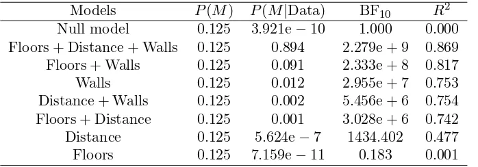
Table 2. Model comparison.

Models P(M) P(M|Data) BF10 R2

Null model 0.125 3.921e−10 1.000 0.000

Floors + Distance + Walls 0.125 0.894 2.279e + 9 0.869

Floors + Walls 0.125 0.091 2.333e + 8 0.817

Walls 0.125 0.012 2.955e + 7 0.753

Distance + Walls 0.125 0.002 5.456e + 6 0.754

Floors + Distance 0.125 0.001 3.028e + 6 0.742

Distance 0.125 5.624e−7 1434.402 0.477

Floors 0.125 7.159e−11 0.183 0.001

Table 2 lists all 2p possible models’ combinations wherepis the number of explanatory variables. A total of 8 models are considered in this study with BF10 compared to the null model in the fifth column where 6 of these models have extremely high BF10 values. BF10 of the null model is equal to 1 since M1 = M0, and it is considered a better model candidate than a single “Floors” explanatory variable model. Hence, the posterior probability is used to pick and choose from multiple candidates with high BF as:

P(M_i|Data) = P(Data|Mi)P(Mi) k

j=1

P(Data|M_j)P(M_j)

wherekis the number of candidate models. The third column in Table 2 shows the posterior probability for candidate models, here we only consider the top 6 models with BF higher than 150.

Bayesian Information Criterion (BIC) is another strategy used to select and validate predictor variables to be used in the model. This technique leverages the model’s likelihood and the size of the data set for parameters selection as follows:

BIC = ln (n) (p+ 1)−2 ln

ˆ L

(10)

wherenis the number of observations in the data set,pthe number of parameters, and ˆLthe maximum likelihood value. Table 3 shows the marginal inclusion probability for the Bayesian model predictors (Floors, Distance and Walls) in addition to the intercept. It is clear that all predictors have a high inclusion probability that exceeds 0.5 withp(Floors) = 0.986,p(Distance) = 0.897 andp(Walls) = 0.999 indicating the contribution of each predictor on the final model as shown in Figure 1 using the Bayesian Adaptive Sampling (BAS) package forR [15].

Table 3. Posterior summaries of coefficients.

Coefficient Mean SD P(incl) P(incl—data) BF_inclusion

Intercept 65.488 1.187 1.000 1.000 1.000

Floors 15.773 3.338 0.500 0.986 71.856

Distance 1.252 0.396 0.500 0.897 8.703

Walls 6.700 1.352 0.500 0.999 840.953

0.0

0.2

0.4

0.6

0.8

1.0

Marginal Inclusion Probability

Intercept

Floors

Distance

Walls

Figure 1. The marginal inclusion probability for three variables in addition to the intercept.

23.295 20.983 18.975 17.07 16.477 2.676 Model Rank

Log Posterior Odds Walls

Distance Floors Intercept

1 2 3 4 5 6 7

Figure 2. Model rank for all possible combinations.

40 50 60 70 80 90

-15

-10

-5

0

5

10

15

Predictions under BMA

Residuals

bas.lm(RSSI ~ .) Residuals vs Fitted

5 25

4

Figure 3. Residuals vs. fitted values.

4. DATA COLLECTION AND RESULTS

The data are collected using a custom made PC application for wireless interface [16] in a two-storey building as shown in Figure 4. A user carrying a PC collects data at random location points. The used data set contains 30tuples collected at random location points in a two-storey building [17]. 21 of these tuples are recorded in the first floor of the testbed and 9 in the second floor.

Each tuple comprises six variables,x_i, y_i, f l_i, D_i, P r_i and w_i. The model is set as:

P r_i=α+β1xfl_i+β2xDi +β3xwi+i (11)

where P r_i refers to the received power in dBm; f l_i represents the number of floors between the transmitter and receiver; D_i is the Euclidean distance in meters between the location points and the APs; w_i is the number of walls separation between transmitter and receiver; and_i is the error term of theith location point from the Access Point (AP). From Equation (11), the distanceD_i is:

D_i=

(a) (b)

Figure 4. Floor maps for the wireless communication center at Universiti Teknologi Malaysia. (a) First floor. (b) Second floor.

(a)

(b)

(c)

wherex_i and y_i are the coordinates of theith location point, and X and Y are the coordinates of AP. The error term_i is assumed to be Independent and Identically Distributed (iid) with common variance σ2 _as:

_iiid∼Normal (0, τ) (13)

From Equation (11), α, β1, β2 and β3 are the priors for the multiple regression model drawn from a normal distribution with means centered at parameters a, b1, b2 and b3, and τ is Gamma prior distribution for the precision:

α, β1, β2, β3 ∼Normal ((a, b1, b2, b3), τ) (14)

τ ∼Gamma (g1, g2) (15)

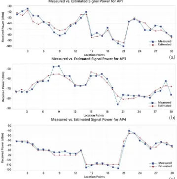
The BAS package for R which provides a predict function using Bayesian Model Averaging (BMA) is used to test the performance of the proposed model. Three models are built for three individual APs replicating distinct indoor environments. Each aforesaid model is supplied with a Zellner-Siow Cauchy prior and a uniform prior. Figure 5 shows the measured and estimated received powers at all location points from AP1, AP3, and AP4, respectively.

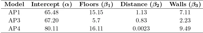
Figure 6 shows the Cumulative Distribution Function (CDF) of estimation error for all APs where each model is based on data collected from that particular AP. The average of estimation error is 4.87 dB for AP1, 3.06 dB for AP3, and 3.55 dB for AP4. The marginal posterior values for coefficientsα,β1,β2, and β3 are listed in Table 4 where the received power can be estimated by substituting the values for each coefficient listed in the table with their associated variables, x_fli,x_Di, and x_wi at theith location point. Eitherβ1 orβ3will be ignored if the transmitter and receiver are at the same floor (i.e.,xfli = 0), or there is a direct LoS between the AP and the location point (i.e., x_wi = 0).

Figure 6. CDF of estimation error.

Table 4. Marginal posterior summaries of coefficients.

Model Intercept (α) Floors (β₁) Distance (β₂) Walls (β₃)

AP1 65.48 15.15 1.13 7.11

AP3 67.20 5.7 0.83 2.23

AP4 80.11 16.11 0.0023 9.49

Average estimation error

1SM = 20.38 dB MWM = 11.16 dB LAM = 10.25 dB Proposed Model = 4.87 dB

Figure 7. Boxplots of estimation error for the proposed model vs. 1SM, MWM and LAM.

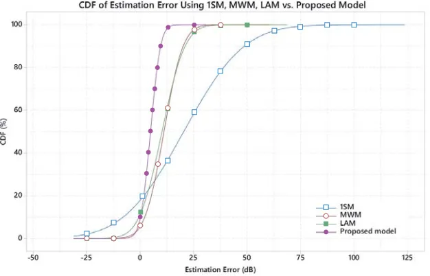
Figure 8. CDF of estimation error for the proposed model versus 1SM, MWM and LAM.

substitute for floors effect. The average estimation error for 1SM is 20.38 dB and 11.16 dB for MWM and 10.25 dB for LAM in comparison with average estimation error of 4.87 dB for the proposed model. The attenuation coefficientαfor LAM model is set to 2.8. Wall Attenuation Factor (WAF) and FAF in MWM model are set to 7 dB and 20 dB, respectively. Note that MWM and LAM perform similarly in terms of average estimation error, but this does not apply to the error variance for both models where variance for MWM is 49.11 dB and 70.93 for LAM. This is also visible by the CDF plot for all models in Figure 8.

Figure 9. CDF of estimation error for AP3 and AP4 based on AP1 model.

5. CONCLUSION

The purpose of the current study is to design a Bayesian model for predicting the signal power in indoor environments. The proposed model estimates the received power at the receiver in a complex indoor environment. The parameters of the Bayesian multiple regression model are validated using different strategies to ensure their suitability to the model.

ACKNOWLEDGMENT

This research was supported by the Deanship of Scientific Research, Majmaah University, Majmaah, 11952, Kingdom of Saudi Arabia (Contract No. 38/105).

REFERENCES

1. Madigan, D., E. Elnahrawy, R. P. Martin, W. H. Ju, P. Krishnan, and A. S. Krishnakumar, “Bayesian indoor positioning systems,” Proceedings — IEEE INFOCOM, Vol. 2, 1217–1227, 2005. 2. Al-Ahmadi, A., A. I. A. Omer, M. R. Kamarudin, and T. A. Rahman, “Multi-floor indoor positioning system using Bayesian graphical models,” Progress In Electromagnetics Research B, Vol. 25, 241–259, 2010.

3. Xu, H., Y. Ding, P. Li, R. Wang, and Y. Li, “An RFID indoor positioning algorithm based on Bayesian probability and K-Nearest Neighbor,” Sensors, Vol. 17, No. 8, 1806, Switzerland, Aug. 2017.

4. Zaman, T., E. B. Fox, and E. T. Bradlow, “A Bayesian approach for predicting the popularity of tweets,” Annals of Applied Statistics, Vol. 8, No. 3, 1583–1611, 2014.

5. Steorts, R. C., R. Hall, and S. E. Fienberg, “A Bayesian approach to graphical record linkage and deduplication,”Journal of the American Statistical Association, Vol. 111, No. 516, 1660–1672, 2016.

6. Campisi, P. and K. Egiazarian,Blind Image Deconvolution: Theory and Applications, 1st Edition, CRC Press, 2007.

8. Damosso, E., “Digital mobile radio towards future generation systems: COST action 231,” European Commission, 1999.

9. Tarng, J. H. and T. R. Liu, “Effective models in evaluating radio coverage on single floors of multifloor buildings,”IEEE Transactions on Vehicular Technology, Vol. 48, No. 3, 782–789, 1999. 10. Lawton, M. C. and J. P. McGeehan, “The application of a deterministic ray launching algorithm

for the prediction of radio channel characteristics in small-cell environments,”IEEE Transactions on Vehicular Technology, Vol. 43, No. 4, 955–969, Nov. 1994.

11. Herring, K. T., J. W. Holloway, D. H. Staelin, and D. W. Bliss, “Path-loss characteristics of urban wireless channels,” IEEE Transactions on Antennas and Propagation, Vol. 58, No. 1, 171–177, Jan. 2010.

12. Malnar, M. and N. Jevtic, “Novel multi-room multi-obstacle indoor propagation model for wireless networks,” Wireless Personal Communications, Vol. 102, No. 1, 583–597, Sep. 2018.

13. Rouder, J. N. and R. D. Morey, “Default Bayes factors for model selection in regression,”

Multivariate Behavioral Research, Vol. 47, No. 6, 877–903, Nov. 2012.

14. Posada, D. and T. R. Buckley, “Model selection and model averaging in phylogenetics: Advantages of akaike information criterion and Bayesian approaches over likelihood ratio tests,” Syst. Biol., Vol. 53, No. 5, 793–808, Oct. 2004.

15. Clyde, M., “BAS: Bayesian variable selection and model averaging using Bayesian adaptive sampling,” R package version 1.5.3, 2018.

16. Al-Ahmadi, A. S., T. A. Rahman, M. R. Kamarudin, M. H. Jamaluddin, and A. I. Omer, “Single-phase wireless LAN based multi-floor indoor location determination system,” 2011 IEEE 17th International Conference on Parallel and Distributed Systems, 1057–1062, IEEE, Dec. 2011. 17. Al-Ahmadi, A. and T. A. Rahman, “One stage indoor location determination systems,” New

Approach of Indoor and Outdoor Localization Systems, F. B. Elbahhar and A. Rivenq, editors,