Study on Operating Status of Overhead Transmission Lines Based on Wind Speed Variation

(1)

Study on Operating Status of Overhead Transmission Lines

Based on Wind Speed Variation

Yang Mo1, Xiaofeng Zhou2, Yanling Wang1, *, and Likai Liang1

Abstract—In the spatial dimension, the variation of the wind speed along the overhead transmission line makes the conductor temperature and line parameter show a nonuniform distribution characteristic, which has an important inﬂuence on the operating status of the system. In order to describe the actual situation more accurately, a line division model based on the wind speed variation along the line is proposed. This paper proves the application value of the model by using a typical 4-bus system. From the two aspects of the power ﬂow and maximum power transmission capacity, we contrast the line division model with the traditional models, indicating that the division model is closer to the actual situation of the system.

1. INTRODUCTION

The meteorological conditions along the overhead transmission line are important factors affecting the operating status of the line. However, the traditional static thermal rating uses conservative meteorological data to determine the operating limits of the line [1]. For example, wind speed is designed to be 0.5 m/s, and ambient temperature is designed to be 40◦C. Some studies have been improved by presenting seasonal static thermal rating [2]. The calculation result is also very different from the actual situation. Dynamic thermal rating takes into account the real-time changes in meteorological conditions [3, 4], and to a certain extent, the accuracy of the calculation result is improved. However, the changes of the line in the spatial dimension are usually not taken into account. The model still uses a single lumped parameter, and its result is still different from the actual situation, especially for long-distance transmission lines.

Due to the complexity of geographical location where the transmission lines pass through, meteorological conditions, such as wind speed, temperature, eﬀectively vary with the line location. For example, the wind speed varies greatly along the transmission line of the mountain outlet and the transmission line of southern coastal area where typhoons often occur [5, 6]. The conductor temperature is aﬀected by the meteorological conditions, and the line parameters show a nonuniform distribution characteristic [7].

The wind is one of the meteorological conditions, mainly acting on the conductor convected-heat loss [8]. Wind speed is the main factor aﬀecting the operation status of the transmission line [9], and an in-depth study of wind speed on the system is necessary.

According to the changes of wind speed along the transmission line, this paper uses three kinds of wind speed models. The average model and the weighted average model adopt the traditional mathematical method to establish a single lumped parameter model of the transmission line [10]. Using these two models, the accuracy of the results is improved, but it still has a certain gap from the actual situation. At present, for the analysis of the spatial dimension of overhead transmission lines, some

Received 26 July 2017, Accepted 14 September 2017, Scheduled 18 September 2017

* Corresponding author: Yanling Wang ([email protected]).

1 _{School of Mechanical, Electrical and Information Engineering, Shandong University (Weihai), Weihai, Shandong 264200, China.} 2

(2)

papers have begun to apply the nonuniform distribution parameter model to solve the problem. In [11], the transmission line is divided into segments of equal length. In [7] and [10], the transmission line is divided by the division model based on ambient temperature. On the basis of these studies, this paper proposes a line division model based on the wind speed along the line, dividing the line into multiple segments. According to diﬀerent locations of the weather data, we determine the wind speed of each segment, and then the accurate conductor temperature and line parameters are obtained for each segment.

In order to verify the accuracy of the line division model based on the wind speed, this paper presents a 4-bus test system to ﬁnd the operation data of the system under normal weather conditions and extreme weather conditions. In addition, we analyze the system power ﬂow and the maximum power transmission capacity through a 4-bus test system.

Section 2 describes the relationship among wind speed, conductor temperature and line parameters. In Section 3, three models are proposed for the wind speed change along the line. In Section 4, we propose a 4-bus test system and make a detailed comparison of the results of the three models. Section 5 summarizes the paper and makes a brief explanation of the future research.

2. BACKGROUND

This section discusses the relationship among wind speed, conductor temperature and line parameters. Firstly, the inﬂuence of conductor temperature on the line parameters is discussed. Then, the inﬂuence of the wind speed on the conductor temperature is discussed. Finally, the mechanism of the wind speed on the overhead transmission line is determined.

2.1. Relationship between Conductor Temperature and Line Parameters

Overhead transmission lines have four main parameters: series resistance r, series reactance xL, shunt

susceptanceb and shunt conductanceg. These parameters mainly depend on the characteristics of the conductor material, the surrounding electric ﬁelds and magnetic ﬁelds, and the geographical location of the transmission line [12].

The resistance and reactance are linear functions of the conductor temperature, as shown in Eqs. (1) and (2):

r(Tc) = r(T0)·[1 +α(Tc−T0)] (1)

xL(Tc) = xL(T0)·[1 +β(Tc−T0)] (2)

where T0 is the reference temperature (it is usually 20◦C in the power system), Tc the conductor

temperature, and αand β are the temperature coeﬃcients of resistance and conductance, respectively, depending on the physical properties of the conductor.

Line shunt susceptance is usually considered constant, because the eﬀect of temperature changes on line charging is usually negligible, without considering external environmental conditions, such as humidity. In addition, since the actual line operating voltage is lower than the corona critical voltage, it can be assumed that no corona occurs, so the shunt conductance is often taken as zero.

Through the above analysis, the inﬂuence of conductor temperature on the line parameters is mainly reﬂected in the change of resistance and reactance.

2.2. Relationship between Wind Speed and Conductor Temperature

Under steady-state conditions, the heat balance equation for the conductor is expressed as:

qc+qr=I2r+qs (3)

where qc is the convected heat loss, qr the radiated heat loss, I the current through the transmission

line,r the resistance at the corresponding conductor temperature, andqs the solar heat loss.

In the CIGRE standard, convected heat loss qc can be further expressed as:

qc=πλf(Tc−Ta)B1

Dρfvw

μf

_n

(3)

whereTa is the ambient temperature,λf the thermal conductivity of the air,Dthe conductor diameter,

ρf the air density, μf the air viscosity coeﬃcient, andvw the wind speed.

Under conditions of constant ambient temperatureTa, becauseλf andμf are functions of conductor

temperatureTc,qccan be seen as a function of conductor temperatureTc and wind speedvw.

In the line actual operation, with the increase in wind speed, the conductor temperature will drop, so the line impedance also decreases, thus it will aﬀect the system power ﬂow and the line maximum power transmission capacity.

3. MODELS COMBINED WITH WIND SPEED

This section describes three models for handling wind speed variations along overhead transmission lines. All wind speed information is based on the measurement devices installed along the transmission line, or the nearby weather stations. Model 1 and model 2 treat the line as a single lumped parameters model. The model 3 is the most appropriate description of the actual situation, and it is the focus of this paper. The model 3 divides the line into multi-segments lumped parameters. Please note that, in the limit, the line parameters show the nonuniform distribution characteristics.

3.1. Average Model

In this model, for the wind speed changes in the transmission line, taking the average wind speed value vavg at the beginning and end of the line, to approximate the entire line,vavg can be determined by the

following formula:

vavg =

vbeg+vend

2 (5)

wherevbeg is the wind speed at the beginning of the line, andvend is the wind speed at the end of the

line.

3.2. Weighted Average Model

For wind speed changes in the transmission lines, we use the weighted average vwavg to represent the

entire line, and the weighted average method is based on the wind speed measurement points along the line to determine:

vwavg =

N−1

i=1

v_i+v_i+1

2

× Δxi,i+1

l

(6)

whereN is the total number of wind speed measurement points;iis the wind speed measurement point (i= 1. . . N) on the line;v_i is the wind speed value at the measurement pointi; Δx_i,i+1 is the the line

length between the measurement point iand its next measurement point i+ 1; l is the total length of the line.

3.3. Line Division Model Based on Wind Speed

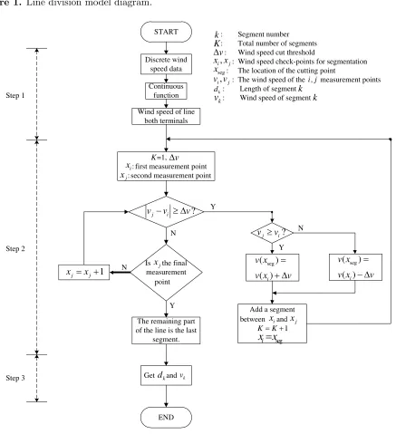
This study assumes that other weather parameters (such as ambient temperature, wind angle, sunshine) along the line are constants. In this paper, a wind speed-based line division model is proposed. The model diagram is as follows.

In Figure 1, k is the segment number, K the total number of segments, v_k the wind speed for segment k, d_k the length of segment k, Z_k the series impedance for segment k, and Y_k the shunt admittance for segment k. V1 and V2 are the beginning and end voltages of the line. I1 andI2 are the

beginning and end currents of the line.

(4)

+

−

+

1( , )1 1

Z d v Z d v2( 2, 2) ZK(dK,vK)

1( )1

Y d Y d2( 2) Y dK( K)

2 k= 1

k= k=K

2 V 2 I 1 V 1 I −

Figure 1. Line division model diagram.

START

=1,

: first measurement point : second measurement point

Is the final measurement

point

Get and

END

Add a segment between and Discrete wind

speed data

Continuous function

Wind speed of line both terminals Y N N Y Y N : Segment number : Total number of segments

: Wind speed cut threshold

: Wind speed check-points for segmentation : The location of the cutting point

: The wind speed of the , measurement points : Length of segment

: Wind speed of segment

The remaining part of the line is the last

segment. k v Δ , i j x x , i j v v k d k v 1 j j

x = +x

?

j i

v − ≥ Δv v

?

j i

v ≥v v Δ i x j x j x k d k k i j K i

x x_j

1 K= +K

seg

i

x x

=

K

seg x

seg

( )

( )_i

v x

v x v = − Δ

seg

( )

( )_i

v x

v x v = + Δ k v Step 1 Step 2 Step 3

Figure 2. Division model algorithm ow chart.

(5)

3.3.1. Step 1): Get the Wind Speed Distribution

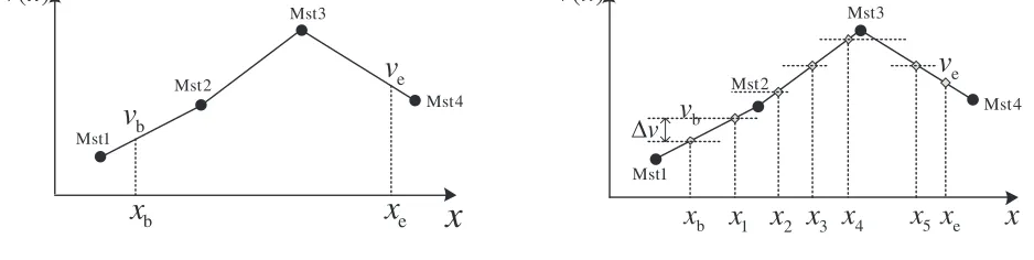
It is assumed that the wind speed changes linearly between any two measurement points along the transmission line, and the wind speed distribution can be determined by each measurement point. Taking into account the actual line, there may be no measuring device at the beginning and end of the line. So we generally consider that the ﬁrst and last measurement points are outside the beginning and end of the line. The discrete wind speed data can be approximated to obtain a continuous type function. The independent variable of the function is the line distance x and the outcome variable is the wind speed v along the line. Figure 3 shows a typical example. The line has four measurement points. The wind speed shows a linear change between each two adjacent measurement points, and the ﬁrst and last measurement points are outside the beginning and end of line. From above, we get a continuous functionv(x) of distancex.

In particular, the wind speed values at the beginning and end of the line are determined according to the following formula:

v_m−v v_m−v_n =

x_m−x

x_m−x_n (7)

where v_m and v_n are the measured wind speed values at both terminals of the points to be measured. x_m and x_nare the position at both terminals of the points to be measured. Respectively, substitutex_b and x_e to get the wind speed v_b and v_e of line both terminals.

e

x

_x

( )

v x

Mst1

Mst2

Mst3

Mst4

b

v

e

v

b

x

Figure 3. Wind speed function.

x

( )

v x

Mst1

Mst2

Mst3

Mst4

4

x

3

x

2

x

1

x

v

Δ

b

x

5

x

e

b

v

e

v

Figure 4. The wind speed distribution after division.

3.3.2. Step 2): Divide the Wind Speed Along the Line

After obtaining the complete wind speed function, we need to set a wind speed threshold Δv to divide the function. From the beginning of the line, towards the end of the line, when the wind speed change reaches the threshold Δv, set the division point. Take the beginning of the line as an example. At the wind speed reachedvb+ Δv, set the division pointx1, and then starting with pointx1, when the wind

speed reaches v(x1) + Δv, set the division point x2. In addition, when dropping along the line, the

wind speed is used to subtract the threshold, and so on until the ﬁnal division point is obtained, and the residual line wind speed change reaches the threshold value at the last segment. After division, the wind speed distribution is shown in Figure 4.

3.3.3. Step 3): Find the Parameter Values for Each Segment

After the completion of the line division, the division point of the wind speed has been determined, and then we need to obtain the segmented wind speed after division. In this step, we use the weighted average method shown in formula (6). It is worth noting that the data in this model are not limited to wind speed measurement points, and instead, it is based on the wind speed known points, including the measurement points, division points and both terminals of line.

After obtaining the wind speed value of each division point, we can get the corresponding position x by taking formula (7), then the length of each segment can be determined by formula (8):

(6)

wherex_k is the starting position and x_k+1 the stop position.

For each segment of the line, the wind speed v_k, other meteorological parameters and current are taken into the heat balance Equation (3) and the power ﬂow equation for iterative solution, and we can get the conductor temperatureT_ck. Series impedance Z_k and shunt admittance Y_k can be determined by conductor temperatureT_ck and lengthd_k of each segment.

Model 1 and model 2 are the traditional models. The calculation results are diﬀerent from the actual situation to a certain degree. The accuracy of model 3 will be shown in the next section.

4. CASE STUDY

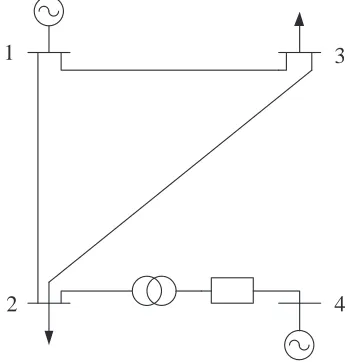
In order to illustrate the application value of the wind speed-dependent line division model proposed in this paper, a simple 4-bus system in various scenarios under diﬀerent models is analyzed as follows. The purpose is to reveal the accuracy of the model, and the system structure is depicted in Figure 5. The transmission lines are arranged in a certain way in this test. In this study, we select the LGJ-400/50 model of aluminium conductors steel-reinforced to test. Parameter settings are as follows: the resistance is 0.0849 Ω/km at 40◦C; the reactance is 0.4366 Ω/km at 40◦C; the susceptance is 2.815×10−6S/km; the resistance and reactance temperature coeﬃcients are 0.0039 Ω/◦C.

1

2

3

4

Figure 5. 4-bus system structure diagram.

The lengths of branches 1-2 and 1-3 are both 150 km, and length of branch 2-3 is 200 km. We set the reference voltage at 220 kV, the reference capacity is 100 MVA. The system structure is shown below. We use a power-ﬂow solver coded in Matlab to build the system, and analyze the system power ﬂow and the maximum power transmission capacity.

Base Case — In order to further compare the accuracy of the three methods, we set the normal weather conditions as the base case and get the result from the system in the base case as the base value. In the power system, an ambient temperature of 40◦C and a wind speed of 0.5 m/s are usually assumed under the base case [7, 14]. The parameters of the line under the base case are shown in Table 2.

High windy scenario — An ambient temperature of 40◦C and a wind speed of 0.5 m/s are assumed, and bus 3 is aﬀected by the extreme weather, such as in a storm, its wind speed suddenly rising to 20 m/s. Aﬀected by the weather, the wind speed shows a nonuniform distribution along branches 1-3 and 2-3. The overall system ambient temperature remains constant.

In order to simplify the problem, it is assumed that the wind speed measurement points are set at both terminals and the point of trisection of the branches 1-3 and 2-3. Measurement point position and measured wind speed are set as shown in Table 1. x1−3 and x2−3 are the distance between the

(7)

Table 1. Measurement point position and measured wind speed.

MST Point x1−3 (km) x2−3 (km) Wind Speed (m/s)

1 0 0 0.5

2 50 66.67 15.5

3 100 133.34 25

4 150 200 20

Model 1 (average model) — branches 1-3 and 2-3 are aﬀected by the storm. The wind speed is calculated by formula (5), and the average value is 10.25 m/s. Then the wind speed distribution of branches 1-3 and 2-3 is represented by a single meteorological value.

Model 2 (weighted average model) — similar to model 1, the weighted average wind speed of lines 1-3 and 2-3 is 16.92 m/s, calculated by formula (6) in this model.

Model 3 (line division model based on wind speed) — considering the accuracy of the model and the system size minimization constraint, we set the wind speed threshold Δv to 5 m/s. Branch 1-3 is divided into ﬁve segments: 1-5, 5-6, 6-7, 7-8 and 8-3, and branch 2-3 is divided into ﬁve segments: 2-9, 9-10, 10-11, 11-12 and 12-3. There is a 12-bus system after completing the division.

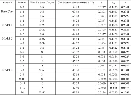
We can get the wind speed values in the above three models. The conductor temperature can be obtained by the repeated solution of the heat balance equation under the CIGRE standard. The line parameters at the corresponding temperature can be obtained by formulas (1) and (2). The detailed values are shown in Table 2.

Table 2. The parameter values for base case and each model.

Models Branch Wind Speed (m/s) Conductor temperature (◦C) r xL b

Base Case

1-2 0.5 54.23 0.0277 0.1423 0.2044

1-3 0.5 69.48 0.0291 0.1497 0.2044

2-3 0.5 55.93 0.0371 0.1909 0.2725

Model 1

1-2 0.5 54.23 0.0277 0.1423 0.2044

1-3 10.25 46.19 0.0267 0.1383 0.2044

2-3 10.25 43.43 0.0355 0.1827 0.2725

Model 2

1-2 0.5 54.23 0.0277 0.1423 0.2044

1-3 16.92 44.54 0.0267 0.1375 0.2044

2-3 16.92 42.52 0.0354 0.1821 0.2725

Model 3

1-2 0.5 54.22 0.0277 0.1422 0.2044

1-5 3 53.02 0.003 0.0157 0.0227

5-6 8 47.23 0.003 0.0154 0.0227

6-7 13 45.37 0.003 0.0153 0.0227

7-8 18 44.4 0.0047 0.0241 0.0359

8-3 22.58 43.86 0.0131 0.0673 0.1004

2-9 3 47.18 0.004 0.0206 0.0303

9-10 8 44.03 0.0039 0.0203 0.0303

10-11 13 43.02 0.0039 0.032 0.0303

11-12 18 42.49 0.0062 0.032 0.0478

(8)

4.1. System Power Flow Analysis

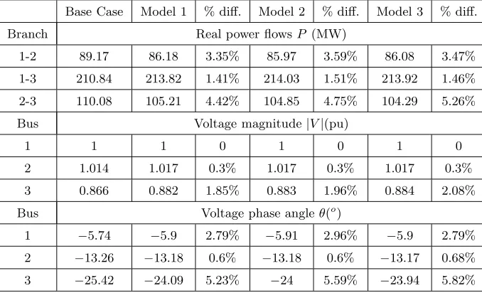
By establishing the system and analyzing the base case and the power flow of the three models, the results are shown in Table 3. The results of each model and the base case are listed in Table 3, including the active powerP and voltage magnitude|V|, voltage phase angleθ. The percentage difference shown in Table 3 is calculated as Eq. (9), and its size reflects the degree of deviation from the base value.

% dif f.=ResultModle 1 2 or 3−ResultBase Case ResultBase Case

×100% (9)

From the active power part, we can see that the three models have the greatest degree of deviation in branch 2-3 with the base case, in which model 1 is 4.42%; model 2 is 4.75%; model 3 is 5.26%. Model 1 is the closest to the base value. The diﬀerence between model 3 and the base value is the largest, and model 2 is in the middle of them. Due to high wind speed design, model 3 is closest to the actual situation. Model 1 is least consistent with the actual situation, and model 2 is between the two.

Table 3. Power-ﬂow results for the system.

Base Case Model 1 % diff. Model 2 % diff. Model 3 % diff.

Branch Real power ﬂowsP (MW)

1-2 89.17 86.18 3.35% 85.97 3.59% 86.08 3.47%

1-3 210.84 213.82 1.41% 214.03 1.51% 213.92 1.46%

2-3 110.08 105.21 4.42% 104.85 4.75% 104.29 5.26%

Bus Voltage magnitude|V|(pu)

1 1 1 0 1 0 1 0

2 1.014 1.017 0.3% 1.017 0.3% 1.017 0.3%

3 0.866 0.882 1.85% 0.883 1.96% 0.884 2.08%

Bus Voltage phase angleθ(o)

1 −5.74 −5.9 2.79% −5.91 2.96% −5.9 2.79%

2 −13.26 −13.18 0.6% −13.18 0.6% −13.17 0.68%

3 −25.42 −24.09 5.23% −24 5.59% −23.94 5.82%

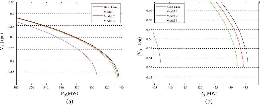
4.2. Maximum Power Transfer Capability

In order to test the maximum power transmission capacity of the system, we gradually increase the load on bus 3. However, we need to ensure that the ratio of active and reactive loads of bus 3 remains constant. The loads of the other nodes remain constant, and the load increment is distributed proportionally to the outputs of the generators. The voltage magnitude of bus 3 will change with the increase of the active load. The change in voltage magnitude with the active load of bus 3 is described in Figure 6, which includes the results of the three models and the base case. The detailed maximum active power values Pmax are listed in Table 4. The maximum power of the base case is 407 MW. The maximum

(9)

Base Case Model 1 Model 2 Model 3

3 Base Case

Model 1 Model 2 Model 3

0.95

0.9

0.85

0.8

0.75

0.7

|V | (pu)

0.65

3

0.69

0.68

0.66

0.65

0.64

0.63

|V | (pu)

0.62

3

0.67

300 320 340 360 380 400 420 440 405 410 415 420 425 430 435

P (MW)₃ P (MW)₃

(a) (b)

Figure 6. (a) PV curves at bus 3. (b) Zoomed-in around the maximum power transfer point.

Table 4. Maximum power transfer point at bus 3 (MW).

Base value Model 1 % diff. Model 2 % diff. Model 3 % diff.

407 432.4 6.24% 434.4 6.73% 435.9 7.1%

5. CONCLUSION AND FUTURE VISION

In the spatial dimension, the wind speed has an important effect on the overhead transmission lines, especially for long-distance transmission lines passing through extreme weather. If the transmission line is set to a single lumped parameter model, the power flow and maximum power transmission capacity are very different from the actual situation. Especially in the high windy area, transmission capacity can be greatly improved. Therefore, it is important to consider the change of wind speed in the spatial dimension to extract the transmission potential of the existing overhead transmission lines.

With regard to the change of wind speed along the overhead transmission line, this paper proposes a line division model based on wind speed. The lines are divided into multiple lumped parameter segments, based on the measurement points. Compared with the average model and the weighted average model, the results obtained by the line division model are closer to the actual value. In the actual grid scheduling, the relevant departments can make more accurate judgments. In the premise of ensuring the safe operation of the grid, we can improve the power transmission capacity to the greatest extent possible.

The following research will take into account the comprehensive meteorological conditions, such as ambient temperature, wind speed, along the overhead transmission lines. The eﬀects of meteorological conditions on the running status of the line will be studied, including the system power ﬂow and maximum power transmission capacity.

ACKNOWLEDGMENT

(10)

REFERENCES

1. Douglass, D. A., “Weather-dependent versus static thermal line ratings,” IEEE Transactions on Power Delivery, Vol. 3, No. 2, 742–753, 1998.

2. Heckenbergerova, J., P. Musilek, and K. Filimonenkov, “Assessment of seasonal static thermal ratings of overhead transmission conductors,” 2011 IEEE Power and Energy Society General Meeting, 1–8, 2011.

3. Douglass, D. A., and A. Edris, “Real-time monitoring and dynamic thermal rating of power transmission circuits,” IEEE Transactions on Power Delivery, Vol. 11, No. 3, 1407–1418, 1996. 4. Fu, J., D. J. Morrow, S. Abdelkader, and B. Fox, “Impact of dynamic line rating on power systems,”

UPEC 2011 46th International Universities’ Power Engineering Conference, 1–5, 2011.

5. Xie, Z. H., “Calculation and analysis of wind speed in design of overhead transmission line in mountain area,”Sichuan Electric Power Technology, Vol. 38, No. 3, 30–32, 2015.

6. Li, T. W., J. H. Zhao, Y. F. Cai, B. Luo, and L. Liu, “Analysis on design wind speed of transmission lines for coastal region of china southern power grid,”Southern Power System Technology, Vol. 9, No. 6, 49–53, 2015.

7. Rahman, M., M. Kiesau, and V. Cecchi, “Investigating the impacts of conductor temperature on power handling capabilities of transmission lines using a multi-segment line model,” SoutheastCon 2017, 1–7, 2017.

8. Zhang, H., X. S. Han, and Y. L. Wang, “Analysis on current carrying capacity of overhead lines being operated,” Power System Technology, Vol. 32, No. 14, 31–35, 2008.

9. Seppa, T. O., “Guide for selection of weather parameters for bare overhead conductor ratings,”

CIGRE Technical Brochure 299, 2006.

10. Cecchi, V., A. S. Leger, K. Miu, and C. O. Nwankpa, “Incorporating temperature variations into transmission-line models,”IEEE Transactions on Power Delivery, Vol. 26, No. 4, 2189–2196, 2011. 11. Cecchi, V., K. Miu, A. S. Leger, and C. Nwankpa, “Study of the impacts of ambient temperature variations along a transmission line using temperature-dependent line models,”Power and Energy Society General Meeting, 1–7, 2011.

12. Grainger, J. J. and W. D. Stevenson, Jr.,Power System Analysis, McGraw-Hill College, 1994. 13. Cecchi, V., M. Knudson, and K. Miu, “System impacts of temperature-dependent transmission line

models,” IEEE Transactions on Power Delivery, Vol. 28, No. 4, 2300–2308, 2013.

14. Zhang, Q. P. and Z. Y. Qian, “Study on real-time dynamic capacity-increase of transmission line,”