A New Technique Based on Grey Model for Forecasting of Ionospheric GPS Signal Delay Using GAGAN Data

(1)

A New Technique Based on Grey Model for Forecasting

of Ionospheric GPS Signal Delay Using GAGAN Data

Ginkala Venkateswarlu1, * and Achanta D. Sarma2

Abstract—The ionospheric GPS signal delay which is a function of TEC plays a major role in the estimation positional accuracy of satellite based navigation systems and detrimental to position estimation, especially in strategic applications. Ionospheric TEC is a function of geographical location (Latitude, Longitude), time, season, etc. In this paper, we propose a system theory based Grey Model (GM(1,1)) which uses past and present data for forecasting TEC (GPS signal delay). In this model, data of nine sequential days from five stations of a GPS Aided Geo Augmented Navigation (GAGAN) system network located at different places representing different latitudes, longitudes and equatorial anomaly regions are used to forecast the 10th day TEC values. The performance of the model is assessed by comparing the statistical parameters such as Standard Deviation (SD) and Mean Square Deviation (MSD). The forecasted results are very encouraging. For all the considered five stations, forecasting is better for post sunset time than day time. Also, the results indicate that SD and MSD values are comparatively higher for Trivandrum (near geomagnetic equator) and Ahmedabad (near the crest of the equatorial anomaly region) stations. These results indicate that the proposed model is useful for forecasting of GPS signal delay both for civil aviation and strategic applications.

1. INTRODUCTION

The Global Positioning System (GPS) is a satellite based navigation system that provides user position, velocity and time information in all weather conditions. Like GPS, other satellite based navigation systems such as GLONASS of Russia, Galileo of Europe, Compass of China and IRNSS of India have come up. In order to receive and utilize signals from these systems, the receiver antenna should have a wide bandwidth and high performance [1]. Characterization of GPS signals is very important in evaluating the overall performance of the navigation system. The propagating GPS signals experience different effects in different environments and need statistical techniques to assess the effects. The satellite signals propagate through various atmospheric layers including ionospheric layers and reach the user receiver. Therefore, the accuracy of the user position is limited by a number of errors including ionospheric time delay of the signals and multipath. The signal may reach the receiver by taking multiple reflections from the surrounding environment resulting in multipath. The effect of multipath can be mitigated by using various adaptive filtering techniques [2]. Forecasting the delay would be very helpful in strategic applications. As the ionosphere is dispersive medium, using a dual-frequency GPS receiver, the delay can be estimated by using the code phase and/or carrier phase measurements. Ionospheric delay depends on Total Electron Content (TEC) along the signal propagation path from satellite to receiver. The TEC is a function of solar radiation, season, day, time of the measurements and receiver location. In the last two decades, several grid models have been proposed to predict the

Received 14 April 2017, Accepted 18 July 2017, Scheduled 2 August 2017 * Corresponding author: Ginkala Venkateswarlu ([email protected]).

1 _{Department of ECE, Vasavi College of Engineering, Hyderabad, India.} 2 _{Department of ECE, Chaitanya Bharathi Institute}

(2)

TEC for GAGAN applications. Sarma et al. (2009) [3] compared the performance of various grid based ionospheric time delay models for GAGAN system. Ratnam et al. (2012) [4] used Spherical Harmonic Functions (SHF) to model ionosphreric time delay for GAGAN TEC network. Srinivas et al. (2016) [5] used Anisotropic IDW with Jackknife Technique to model Ionospheic time delay. However, the grid models are valid only for near realtime applications such as aviation and are meant for the next 5 to 10 minutes [6]. As the data correspond to low/equatorial latitude region, the GPS signals are more susceptible to the ionospheric gradients making the time delay forecasting diﬃcult [7]. The aim of this paper is to predict the GPS signal delay for the immediate following day based on the past and present data by using state of the art forecasting algorithms.

For this type of forecasting/ predicting, several authors proposed various techniques including artificial and statistical techniques. Krankowski et al. (2006) [8] used wavelet analysis for short term forecasting of ionospheric TEC by considering data from European IGS/EPN permanent stations. Neural Network (NN) based models are popularly known as artificial intelligence based models. Tulunay et al. (2006) [9] used NN model to forecast TEC maps using data of Europe centered over Italy. The disadvantage of NN model is that it requires more data and long training period [10]. Therefore, normally for short term time series forecasting, statistical methods are used. Auto Regressive Moving Average, which is a parametric model, was used to forecast the global TEC maps [11]. It is difficult to construct a mathematical model by using conventional linear statistical methods. Exponential Smoothing method, Holt-Winter method, etc. are the prominent existing statistical models for forecasting. Elmunim et al. (2015) [12] considered the GPS data due to UKM station located in Malaysia during May and June, 2010 to forecast ionospheric delay using Holt-Winters models. The results show that the forecasting accuracy of the signal delay using Holt-Winter’s Additive and Multiplicative models was up to 68–92% and 70–93%. In another research paper, the authors considered Indian Regional Navigation Satellite System (IRNSS) VTEC data due to IRNSS receiver located at Hyderabad, India for forecasting [13]. The forecasting accuracy of the Exponential Smoothing method shows up to 89%, Holt-Winters’ Additive method up to 89%, and multiplicative model up to 95%. In this research paper, we used VTEC data due to five GAGAN stations for assessing the forecasting performance using grey model and proved to be better. Therefore, a new model based on system theory is proposed.

In system theory, a system can be described with color that represents the amount of clear information related to that system. A system whose characteristics can be described completely using mathematical equations is known as white system; otherwise, it is called a black box. A flight data recorder may be described by black box. A system that consists of both known and unknown information is called a grey system [14]. For example, the communication systems may be described as white systems and weather systems expressed as grey systems. Grey model was first introduced by Deng [15]. Kayacan et al. (2010) [16] applied different Grey models to forecast United States dollar to Euro parity. In this paper, we use this particular model to predict GPS signal delay using the data taken from five stations namely, Ahmedabad, Bangalore, Delhi, Hyderabad and Trivandrum of Indian GAGAN network.

2. GREY MODEL GM(P, Q)

The grey model is being widely used in various diversified applications, such as scientific, technological, meteorological, transportation applications, and even in financial fields due to its computational efficiency. In this section, we present the salient features of grey model in the context of forecasting TEC.

(3)

these accumulated data to forecast the required TEC data (GPS signal delay) [17].

Consider a sequence X(0) consisting of ‘n’ Vertical TEC (VTEC) data values due to GAGAN station network. X(0) _{is a non-negative sequence of VTEC data. It can be expressed as,}

X(0) = (x(0)(1), x(0)(2), x(0)(3), . . . , x(0)(n)) n≥4 (1)

AGO is used on VTEC data to obtain accumulated sequenceX(1).

X(1) = (x(1)(1), x(1)(2), x(1)(3), . . . , x(1)(n)) n≥4 (2) where,

x(1)(k) = k

i=1

x(0)(i) k= 1,2,3, . . . , n (3)

The grey derivative ofx(1) is denoted as [18]

d(k) =x(0)(k) =x(1)(k)−x(1)(k−1) (4)

The mean value of adjacent data of x(1)(k) is z(1)(k) which can be written as,

z(1)(k) = 0.5x(1)(k) + 0.5x(1)(k−1) k= 2,3, . . . , n (5) In GM(1,1) model, grey diﬀerential equation can be expressed as [15]

x(0)(k) +az(1)(k) =b (6) where, aand bare called sequence parameters.

The GM(1,1) model is a ﬁrst order diﬀerential equation with one variable and can be expressed as,

d(k) +az(1)(k) =b (7)

The variable k= 2,3, . . . , n is a function of time ‘t’, becausekvalue varies with time. Thenx(1)(t) is a time function of x(1). Now Equation (6) can be written as

dx1(t)

dt +ax

(1)₍

t) =b (8)

The procedure for estimation of coeﬃcients aand b is as follows: Equation (6) can be written in the matrix form as (k= 2,3, . . . , n)

⎡ ⎢ ⎢ ⎣

x(0)(2)

x(0)(3)

. x(0)(n)

⎤ ⎥ ⎥ ⎦=

⎡ ⎢ ⎢ ⎣

−z(1)(2) 1 −z(1)(3) 1

. .

−z(1)(n) 1

⎤ ⎥ ⎥ ⎦ ab

(9)

Using the least square method,aand bcan be estimated as,

[ a b ]T =BTB−1BTY (10)

whereY is called data vector, andB is called data matrix and can be deﬁned as,

Y =

⎡ ⎢ ⎢ ⎣

x(0)(2)

x(0)(3)

. x(0)(n)

⎤ ⎥ ⎥

⎦ (11)

B =

⎡ ⎢ ⎢ ⎣

−z(1)(2) 1 −z(1)₍₃₎ ₁

. .

−z(1)(n) 1

⎤ ⎥ ⎥

(4)

The solution of Equation (8) at time kcan be written as

x(1)_p (k+ 1) = x(0)(1)− b

a

e−ak+ b

a (13)

The forecasted value of the original data at time (k+ 1) can be obtained by using grey model and IAGO as,

x(0)_p (k+ 1) = x(0)(1)− b

a

e−ak(1−ea) (14)

3. DATA ACQUISITION

In India, the Indian Space Research Organisation (ISRO) and Airport Authority of India (AAI) have jointly developed a Satellite Based Augmentation System (SBAS) known as GPS Aided Geo Augmented Navigation (GAGAN) system. GAGAN is designed to be interoperable with other international SBAS systems such as US WAAS, European EGNOS and Japanese MSAS. Similar to other international SBAS systems, GAGAN provides additional accuracy, availability and integrity necessary for all phases of flight, enroute through approach for all qualified airports within GAGAN service volume [19]. This GAGAN programme has obtained required certifications for Required Navigation Performance (RNP) 0.1 and Approach Procedure with Vertical guidance (APV) 1.0 Service over Indian Airspace. APV1 service provides APV approaches for selecting runways within India [20].

As a part of GAGAN project, a selected group of 20 TEC stations are deployed at well surveyed locations over widely separated geographical area over India to support ionospheric radio wave propagation studies. These stations are nearly at the centers of 5◦ ×5◦ grids over India. The TEC stations consist of dual-frequency GPS receivers to acquire GPS signals. Space Application Center, ISRO, Ahmedabad, India is responsible for collecting the data from various TEC stations of the GAGAN network.

(5)

The raw GPS data contain 23 parameters. Among them, only seven parameters, namely satellite vehicle number (SV), GPS week number, GPS seconds of the week, elevation angle, azimuth angle, STEC, and user location are used in the analysis. Slant TEC due to various satellites is converted to vertical TEC using standard mapping function corresponding to an Ionospheric Pierce Point (IPP) altitude of 350 kms. All the results are represented in terms of local time.

In order to validate the performance of the proposed model for forecasting the ionospheric GPS signal delay, GAGAN TEC data with 60 seconds sampling interval corresponding to several consecutive days from five TEC stations, namely, Bangalore, Delhi, Hyderabad, Ahmedabad and Trivandrum, are considered (Fig. 1). The first three stations have almost the same longitude but different latitudes. In this way, we can study the performance of the model at different latitudes. The fourth station (Ahmedabad) is near the crest region of the equatorial anomaly, and the fifth station (Trivandrum) is near the geomagnetic equator. Equatorial anomaly region extends up to nearly ±20 degrees from the magnetic equator. It anomaly occurs due to trough in the ionization process in F2 layer at the equator and crests near about 17 degrees in magnetic latitude, and affects the GPS signals [21–23]. The current in the F layer due to horizontal magnetic field increases the ionization in the F layer. The forecasting at these stations will help us to assess the proposed model’s performance in low latitude regions which experience anomaly conditions.

4. RESULTS AND DISCUSSIONS

As the orbital period of the GPS satellite is half of the sidereal day, the following day satellite arrives at the same spot in the orbit nearly 4 minutes early. GPS provides very precise time in the order of nanoseconds and has applications in diversified fields including communication systems, defence applications, electrical power grids, financial transactions, etc. In our analysis, observation time is kept constant, even though the same satellite advances slightly in the orbit as each day progresses. That is, the dataset consists of observations at the same local time even though the IPP position slightly differs [24]. For example, vertical TEC data from a particular satellite at 14:00 Hrs for nine consecutive days are considered in the GM(1,1) model to predict the ionospheric signal delay value at 14:00 Hrs of 10th day. The same procedure is repeated for every minute and for the whole visible period of the satellite. This type of analysis is carried out for several typical solar activity days (0≤kp ≤6). The

kp index is used to express the disturbances in the horizontal component of earth’s magnetic field. Depending on the values of kp index, each day is classified as quiet day (1 < kp < 2), moderate day (2 ≤kp ≤4) and storm day (kp≥5) [25]. Analysis period is categorized as day time and post sunset time to know how the model forecasts during different times of the day. Satellite selection is based on the availability of data throughout the considered time periods. For each plot presented in the figures, both elevation and azimuth angles are indicated at the beginning and end of the plot so that one can appreciate in which direction the signal is propagating through.

Code phase measurements are easy to do, and their accuracy is less, whereas Carrier phase measurements are more precise but diﬃcult to do. Either of these measurements or combination of these measurements are essential for position estimation.

In order to predict VTEC data, coefficients a and b are chosen for each of the five cases and are estimated by considering the data of every epoch and using least square method. For example, at Delhi station during day time a particular Satellite Vehicle (SV) is visible for about five hours. With a sampling period of one minute, a total of 300 epochs data can be obtained. The coefficients are estimated for each epoch (Equation (10)) and used for forecasting purpose. The same procedure is followed for the remaining four cases (Hyderabad, Bangalore, Ahmedabad and Trivandrum), and the results are very encouraging.

4.1. Delhi

4.1.1. Day Time TEC Forecasting

(6)

9 10 11 12 13 14 10 15 20 25 30 35 40 45 50 55 60 65 70 75 80

kp = 2

Local Time ( Hrs)

TECU

For ec as te d da ta Or iginal da ta

Dat e: 13- 04- 200 6 SV -6

el :33. 14 az: 177. 66

el :1 7. 08 az :307 .1 8

9 10 11 12 13 14 15

20 25 30 35 40 45 50

kp 2

Local Time (Hrs)

TEC

U

Forecas te d data Original dat a

Da te :11- 04-2006 SV -6

el:33. 03 az:175.82

el:17. 14 az: 319 .67

12 13 14 15 16 17 18

30 35 40 45 50

kp 4

Lo ca l Time ( Hrs)

TE

C

U

Forecas te d da ta Or igin al dat a

SV -1 5

Da te :10- 04- 200 6

el :1 7. 13 az:3 17 .63

el :3 2. 82 az:1 56 .02

12 13 14 15 16 17 18

30 35 40 45 50

kp 6

TE C U Forecasted data Original data Date:09-04-2006 SV-18 el:50.32 az:245.44 el:23.88 az:79.90

8 9 10 11 12 13 14

15 20 25 30 35 40

k p = 0

TEC

U

Forecas te d data

Origin al data

SV-30

el:29. 57 az: 185 .45

el:17. 15 az:324. 23

Da te :08- 04- 2006

(a) (b)

(c) (d)

(e)

≤

≤ _≤

Figure 2. (a)–(e) Forecasted TEC for the day time due to Delhi, Hyderabad, Bangalore, Ahmedabad and Trivaudrum stations using GM(1,1) model.

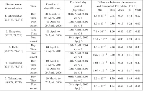
TEC follows the measured TEC (Fig. 2(a)). The SD and MSD values are 0.36 and 0.38 corresponding to day time TEC data (Table 1).

4.1.2. Post Sunset TEC Forecasting

(7)

Table 1. Comparison of diﬀerent stations data.

Station name

& coordinates Time

Considered days (09 days)

Predicted day period

(Kpvalue)

Diﬀerence between the measured and forecasted TEC data (TECU)

Min Max Mean SD MSD

1. Ahmedabad

(23.5◦N, 72.5◦E)

Day Time

31 March to 08 April, 2006

09th April, 2006

kp≤6 1.4×10

−3 _2.35 _0.58 _0.44 _0.52

Post sunset

01 April to 09 April, 2006

10th April, 2006

kp≤3 1.9×10

−4 _0.89 _0.16 _0.22 _0.07

2. Bangalore

(13◦N, 77.5◦E)

Day

Time 01 April to

09 April, 2006

10th April, 2006

kp≤4 7.3×10

−3 _1.60 _0.39 _0.37. _0.29

Post sunset

10th April, 2006

kp≤3 1.16×10

−4 _0.98 _0.30 _0.23 _0.14

3. Delhi

(28.7◦N, 77.2◦E)

Day

Time 04 April to

12 April, 2006

13th April, 2006

kp= 2 1.3×10

−3 _2.46 _0.51 _0.36 _0.38

Post sunset

13th April, 2006

kp≤4 2.35×10

−4 _0.40 _0.14 _0.11 _0.03

4. Hyderabad

(17.5◦N, 78.5◦E)

Day Time

11th April, 2006

kp≤2 1.03×10

−4 _1.45 _0.54 _0.34 _0.40

Post sunset

10th April, 2006

kp≤3 1.07×10

−4 _0.99 _0.11 _0.17 _0.04

5. Trivandrum

(8.5◦N, 77◦E)

Day

Time 30 March to

07 April, 2006

08th April, 2006

kp= 0 2.2×10

−3 _1.79 _0.64 _0.49 _0.64

Post sunset

08th April, 2006

kp≤1 4.3×10

−3 _1.94 _0.59 _0.40 _0.51

2006 (kp= 4 to 4−). The forecasted TEC follows the measured TEC closely (Fig. 3(a)). The SD and MSD values are 0.11 and 0.03 corresponding to post sunset TEC (Table 1).

4.2. Hyderabad

For forecasting TEC data corresponding to 2 April to 10 April 2006 are considered. Satellite (SV-6) is visible for about 5 Hrs from 10:00 Hrs to 15:00 Hrs. The TEC data are forecasted for 11 April 2006 (1< kp≤2). The forecasted TEC follows the measured TEC except from 13:00 to 14:30 Hrs (Fig. 2(b)). The maximum deviation between measured and forecasted TEC data is 1:45 TECU. The SD and MSD values are 0.34 and 0.40, respectively (Table 1). This can be explained as follows: All the nine days have diﬀerentkp index values (3 days havekpindex value around 0. One day has about 2. 3 days have around 4. 1 day has around 1. Another day has 5–6) causing the prediction of the 10th day data slightly less accurate.

(8)

18 19 20 21 22 23 0 5 10 15 20 25

kp 4

Loca l Time ( Hr s)

TEC

U

For ec as te d da ta or igi na l da ta el :17. 28

az : 167 .1 3

SV -1 6

Dat e: 13- 04- 200 6

el :31. 38 az :40. 3

18 19 20 21 22 23

5 10 15 20 25 30 35 40

kp 3

Local Ti me ( Hrs)

TECU

Fore cast ed data Origin al data

SV -16 el :17. 29 az:175. 81

el :33. 27 az:34.29 Date :10-04- 200 6

18 19 20 21 22 23

10 15 20 25 30

kp 3

TEC U Forecasted data Original data el:33.51 az:32.98 el:17.08 az:179.54 SV-16 Date :10-04-2006

18 19 20 21 22 23

0 5 10 15 20 25 30 35 40 45 50

kp 3

TEC U Forecasted data Original data Date:10-04-2006 el:18.64 az:164.25 el:33.36 az:39.74 SV-16

18 19 20 21 22 23

10 15 20 25 30

kp 1

TEC U Forecasted data Original data Date:08-04-2006 el :32.16 az:31.79 SV-16 el :17.08 az:184.28 (a) (b) (c) (d) (e) ≤ ≤ ≤ ≤ ≤

Figure 3. (a)–(e) Forecasted TEC for post sunset time due to Delhi, Hyderabad, Bangalore, Ahmedabad and Trivaudrum stations using GM(1,1) model.

4.3. Bangalore

For this station, SV-15 is visible for about 5 Hrs from 13:00 Hrs to 18:00 Hrs. Data corresponding to 9 days are considered (1 April to 9 April, 2016) as input to the proposed model and forecasted TEC (GPS signal delay) values on 10 April which is a moderate day (2< kp≤4) value.

(9)

to 17.45 Hrs shown in (Fig. 2(c)). This may be due to more variations of the kp index values in the input data to the model (5 days nearly 0–1, 3 days nearly 2–5, 1 day 6–4+). Thekp values on 9 April and 5 April are 6 and 5. The maximum and minimum deviations between measured and forecasted TEC data are 1.6 and 7.3×10−3 _{TECU, and SD and MSD values are 0.37 and 0.29, respectively.}

For the same station and dates, SV-16 is visible for about 5 Hrs from 18:00 Hrs to 23:00 Hrs, and the corresponding data are considered for forecasting.

The TEC data are forecasted for 10 April 2006 (kp = 3 to 3−). The forecasted TEC data follow

the measured TEC data closely except about 18:50 to 19:00 Hrs and 20:25 to 20:70 Hrs (Fig. 3(c)). It is evident from Table 1 that the SD and MSD values are 0.23 and 0.14 in post sunset time, respectively. The post sunset time SD and MSD values are less than day time values.

4.4. Ahmedabad

For this station, SV-18 is visible for about 5 Hrs from 12.00 Hrs to 17.00 Hrs. Data corresponding to 9 days (31 March to 8 April 2006) are considered for forecasting the TEC (GPS signal delay) values on the 10th day (9 April 2006). The forecasted TEC data along with the observed data are shown in (Fig. 2(d)). It can be seen from the ﬁgure that the forecasted TEC data follow the measured TEC data closely. However, towards the end of the satellite pass, there is a slight diﬀerence between the measured and forecasted TEC data. This deviation may be attributed to the following reason:

During the speciﬁed period between 16:00–17:00 Hrs, out of the nine days, seven days have a kp

index in the range of 0–2, and one of the remaining two days has a kp index in the range of 4−to 4 (5 April 2006). The other one day, the kpindex value is in the range of 4− to 1+. On the 10th day on which the values of kpindexes are in the range from 6 to 4+, much higher than the values of the days taken as input to the model. This can be reason for the deviation between the forecasted values and measured value. The SD and MSD values are 0.44 and 0.52 (Table 1).

For the same station, SV-16 is visible for about 5 Hrs from 18:00 Hrs to 23:00 Hrs. As the data of 31 March 2006 are not of good quality, the TEC is forecasted for 10 April 2006. The forecasted values closely follow the measured TEC (GPS signal delay) as shown in (Fig. 3(d)). The SD and MSD values corresponding to post sunset time are 0.22 and 0.07, respectively.

The post sunset time SD and MSD values are less than day time TEC data values because the variation of TEC in night time is less in the absence of solar radiation. From these values, it is evident that GM(1,1) model forecasts the night time TEC data more precisely than that of day time TEC data.

4.5. Trivandrum

For this station, SV-30 is visible for about 5 Hrs from 9:00 to 14:00 Hrs. The input data correspond to 30 March to 7 April 2006. The TEC data (GPS signal delay) are forecasted for 8 April 2006 (kp= 0 to 0+). The forecasted TEC data follow the measured TEC data except from 9.00 Hrs to 10:80 Hrs and from 12:35 to 13:15 (Fig. 2(e)). The kp index of the preceding 9 days varies signiﬁcantly (3 days 0, 2 days 1–2, 2 days 0–1, 2 days 3–5) causing more deviations. The SD and MSD are 0.49 and 0.64.

(10)

18.00 to 18.5 Hrs, 19.00 to 19:70 Hrs and 20.:20 Hrs to 22:37 Hrs. This may be due to more variations in the measured TEC data. During the considered period,Kpindex also varies drastically (2 days nearly 0+, 2 days 0–1, 2 days 1–2, 2 days 1–2+, 1 day 5− to 5+). It is evident from Table 1 that the values of SD and MSD are 0.40 and 0.51.

5. CONCLUSION

Forecasting of GPS signal delay is very important not only for civil aviation applications but also in strategic applications. For forecasting, we propose a technique based on grey model and assess its performance for ionospheric stations located in different places all over India. Data corresponding to five GAGAN stations are used in the proposed technique. From the results, we find that the model performs better for stations (Hyderabad, Bangalore and Delhi) located other than at anomaly crest regions (Ahmedabad) and very near equatorial regions (Trivandrum). Even at Ahmedabad & Trivandrum also, the SD and MSD values are within 0.44 and 0.52, 0.49 and 0.64 respectively. Also, it is found in general night time (SD = 0.11 and MSD = 0.03) that forecasting is better than day time forecasting (SD = 0.34, MSD = 0.40). As India comes under low latitude region, the ionospheric variations are intense and irregular. Even with this type of erratic ionospheric data as input, the grey model shows good performance. Hence, this model is expected to perform well in any other areas.

ACKNOWLEDGMENT

The research work presented in this paper has been carried out under the RESPOND programme of Indian Space Research Organization (ISRO) vide sanction letter no: ISRO/RES/2/399/15-16, dated: 13 July 2015. The authors are grateful to Shri. K. Bandopadhyay and Dr. M. R. Sivaraman, Space Application Centre — ISRO, Ahmedabad for providing the GAGAN data.

REFERENCES

1. Kumar, A., A. D. Sarma, A. K. Mondal, and K. Yedukondalu, “A wide band antenna for multi-constellation GNSS and augmentation systems,” Progress In Electromagnetic Research M, Vol. 11, 65–77, 2010.

2. Yedukondalu, K., A. D. Sarma, and V. Satya Srinivas, “Estimation and mitigation of GPS multipath interference using adaptive ﬁltering,” Progress In Electromagnetic Research M, Vol. 21, 133–148, 2011.

3. Sarma, A. D., D. Venkata Ratnam, and D. Krishna Reddy, “Modelling of low-latitude ionosphere using modiﬁed planar ﬁt method for GAGAN,” IET Radar Sonar Navig., Vol. 3, No. 6, 609–619, 2009, doi: 10.1049/iet-rsn.2009.0022.

4. Venkata Ratnam, D. and A. D. Sarma, “Modeling of low-latitude ionosphere using GPS data with SHF model,” IEEE Transactions on Geoscience and Remote Sensing, Vol. 50, No. 3, March 2012. 5. Satya Srinivas, V., A. D. Sarma, and H. K. Achanta, “ Modeling of ionospheric time delay using anisotropic IDW with Jackknife technique,”IEEE Transactions on Geoscience and Remote Sensing, Vol. 54, No. 1, January 2016, doi:10.1109/TGRS.2015.2461017.

6. Sarma, A. D., N. Prasad, and T. Madhu, “Investigation of suitability of grid-based ionospheric models for GAGAN,”Electron. Lett., Vol. 42, No. 8, 478–479, April 2006.

7. Satya Srinivas, V., A. D. Sarma, A. Supraja Reddy, and D. Krishna Reddy, “Investigation of the eﬀect of ionospheric gradients on GPS signals in the context of LAAS,”Progress In Electromagnetic Research B, Vol. 57, 191–205, 2014.

8. Krankowiski, A., W. Kosek, L. W. Baran, and W. Popinski,“Wavelet analysis and forecasting of VTEC obtained with GPS observations over European latitudes,” Journal of Atmospheric and Solar-Terrestrial Physics, Vol. 67, 1147–1156, 2006.

(11)

10. Jo, T. C., “The eﬀect of virtual term generation on the neural based approaches to time series prediction,”Proceedings of the IEEE Fourth Conference on Control and Automation, Vol. 3, 516– 520, Montreal, Canada, 2003.

11. Prokhorenkov, A. S. and V. Ya. Choliy, “Parametric modeling of global TEC ﬁelds,” Advances in Astronomy and Space Physics, Vol. 2, 85–87, 2012.

12. Elmunim, N. A., A. M. Hashi, and S. A. Bahari, “Comparison of statistical Holt-Winter models for forecasting the ionospheric delay using GPS observations,” Indian Journal of Radio & Space Physics, Vol. 44, 28–34, March 2015.

13. Venkateswarlu, G. and A. D. Sarma, “Performance of Holt-Winter and exponential smoothing methods for forecasting ionospheric TEC using IRNSS data,” 2017 Second IEEE International Conference on Electrical, Computer and Communication Technologies, (IEEE ICECCT 2017) Coimbatore, Tamil Nadu, India, February 22–24, 2017.

14. Deng, J., “Control problems of grey system,”Systems and Control letters, Vol. 1, 288–294, 1982. 15. Deng, J. L., “Introduction to grey system theory,”The Journal of Grey System, Vol. 1, 1–24, 1989. 16. Kayacan, E., B. Ulutas, and O. Kaynak, “Grey system theory-based models in time series

prediction,”Expert Systems with Applications, Vol. 37, No. 2, 1784–1789, March 2010.

17. Lin, Y. and S. Liu, “A historical introduction to grey systems theory,” Proceedings of IEEE International Conference on Systems, Man and Cybernetics The Netherlands, Vol. 1, 2403–2408, 2004.

18. Hua, Q. and X. Yang, “Base a EMD-grey model for textile export time series prediction,” International Journal of Database Theory and Applications, Vol. 6, No. 6, 29–38, 2013.

19. Ramalingam, K., “GAGAN status,” International Civil Aviation Organization, GNSS PANEL, Working Group A and B Meeting, San Antonio, Texas, USA, October 16–25, 2002.

20. http://www.icao.int/APAC/Meetings/2015%20CNSSG19/WP18 India%20AI%205.5%20%20Cer-tiﬁcation%20of%20GAGAN.pdf.

21. Oliveira, A. B. V., T. N. de Morais, and F. Walter, “Eﬀects of equatorial anomaly in the GPS signals,”ION-GNSS-2003, Portland, OR, September 9–11, 2003.

22. De Morais, T. N., A. B. V. Oliveira, and F. Walter, “Global behavior of equatorial anomaly since 1999 and eﬀects on GPS signals,” IEEE Transactions on Aerospace and Electronic Systems, March 2005.

23. Chakraborty, S. K., A. Dasgupta, S. Ray, and S. Banerjee, “Long term observations of VHF scintillations and total electron content near the crest of the equatorial anomaly in the Indian longitude zone,” Radio Sci., Vol. 34, 241–255, 1999.

24. Reddy Ammana, S. and S. Dattatreya Achanta, “Estimation of overbound on ionospheric spatial decorrelation over low-latitude region for ground-based augmentation systems,”IET Radar, Sonar &Navigation, 2016, doi: 10.1049/iet-rsn.2015.0469.