Characterization of the Neural Mechanisms Supporting the Implementation of Cognitive Control in Human Decision Making

MECHANISMS SUPPORTING THE IMPLEMENTATION OF COGNITIVE CONTROL IN HUMAN DECISION MAKING

Thesis by Shabnam Hakimi

In Partial Fulfillment of the Requirements for the Degree of

Doctor of Philosophy

CALIFORNIA INSTITUTE OF TECHNOLOGY Pasadena, California

2014

ACKNOWLEDGEMENTS

During my time at Caltech I have been the lucky recipient of a great deal of kindness and support. John O’Doherty gave me a home, and for his time, expertise, and understanding I am inexpressibly grateful. I am also lucky to have had the mentorship of Ralph Adolphs, who has been a constant source of sage advice. (The first piece of advice Ralph gave me was at SfN in 2007. Rather than approach him to introduce myself, I cowered behind a poster for twenty minutes, totally awestruck. When I finally got up the courage to be late to our appointment, he immediately put me in my place, telling me that I was being ridiculous.)

I must also thank the other members of my committee, Colin Camerer, Pietro Perona, and Shin Shimojo, for their advice, support, and availability. I must also thank Associate Dean of Graduate Studies Felicia Hunt, without whom I would not have made it through graduate school. Thank you, Felicia, for your incredible kindness and for believing in me when I did not.

I would not have survived without my Caltech family, who helped keep me excited about science while gifting me with laughs along the way. Many thanks to my officemates – Alice Lin, Vanessa Janowski, and Cendri Hutcherson – who made living in the lab worthwhile. More thanks to Damian Stanley, whose encouragement and playlist crafting skills helped me to smile when neither of us wanted to. Thank you to Catherine Holcomb for being dedicated as both collaborator and friend. And boundless gratitude to my patient collaborator Todd Hare, who kindly indulged my many questions as we tried to make sense of experiments that didn’t go as planned… Science!

motivated me to work smarter, harder. I am fortunate to know her as a scientist, collaborator, and friend.

To my family and friends: thank you for understanding when weeks passed without a phone call, and for offering kindness and support when I did finally pick up the phone. To my parents: I promise to call and visit more now that this thesis is complete. My mother and father have always been my most ardent supporters, and this Ph.D. belongs as much to them as it does to me.

ABSTRACT

TABLE OF CONTENTS

Acknowledgments ... iii

Abstract ... v

Table of contents ... vii

List of figures and tables ... viii

Nomenclature ... x

... 11

Chapter 1: Introduction ... 19

Chapter 2: Neural changes associated with learned cognitive control ... 59

Chapter 3: Intra-prefrontocortical connectivity in temporal discounting Chapter 4: Individual differences in temporal discounting and the neural representation of ... 94

imagined rewards ... 110

Chapter 5: Conclusions Bibliography ... 113

Appendix A: Response inhibition task instructions ... 127

Appendix B: Imagine task instructions ... 131

LIST OF FIGURES AND TABLES

Figure 2.1. Task design ... 24

Figure 2.2. Behavioral performance by condition across time ... 29

Figure 2.3. Reaction time by performance across conditions ... 30

Table 2.1. Mean reaction time by condition and performance ... 30

Table 2.2. Regions showing greater response for normal contingency compared to reversal trials. . 31

Figure 2.4. Voxels showing differential effects by condition ... 31

Table 2.3. Regions showing greater response for reversal compared to normal contingency trials .. 32

Figure 2.5. Voxels showing linear effects of time for each condition ... 33

Table 2.4. Regions showing positive linear effects of time in normal contingency trials ... 34

Table 2.5. Regions showing negative linear effects of time in reversal trials ... 35

Figure 2.6. Neural main effects of accuracy in normal contingency trials ... 36

Table 2.6. Regions showing differential effects for correct and incorrect normal trials ... 37

Figure 2.7. Voxels more active in correct reversal trials. ... 38

Table 2.7. Regions showing differential effects for correct and incorrect reversal trials ... 39

Figure 2.8. Voxels showing negative linear effects of time in correct reversal trials ... 40

Table 2.8. Regions showing negative linear effects of time in correct reversal trials ... 41

Figure S2.1. Voxels showing differences for normal contingency and reversal trials when controlling for performance ... 47

Table S2.1. Regions activated for the contrast [NC - NI - RC + RI] ... 48

Figure S2.2. Voxels significantly activated for the contrast [RC - RI - NC + NI] ... 49

Table S2.2. Regions activated for the contrast [RC - RI - NC + NI] ... 50

Figure S2.3. Voxels activated for the contrast [NC - NI + RC + RI] ... 51

Table S2.3. Regions activated for the contrast [NC - NI + RC + RI] ... 52

Figure S2.4. Voxels showing linear effects of time for incorrect reversal trials ... 53

Table S2.4. Regions exhibiting linear change in response over time for incorrect reversal trials ... 54

Figure S2.5. Voxels showing a linear increase in activation for correct normal contingency trials over time ... 55

Table S2.5. Regions exhibiting linear increase in response over time for correct normal contingency trials ... 56

Figure S2.6.Voxels showing a linear increase in activation for incorrect normal contingency trials over time ... 57

Table S2.6. Regions exhibiting linear increase in response over time for incorrect normal contingency trials ... 58

Figure 3.1. Task design and behavioral data ... 64

Figure 3.2. Increased activity in left dlPFC when choosing to accept larger, delayed rewards after controlling for subjective value (p < 0.05, SVC) ... 70

Figure 3.3. Ventral striatum region positively correlated with dSV in GLM-1 (p< 0.05, WBC) ... 71

Figure 3.4. Areas correlated with the rdSV regressor from GLM-2 voxels shown in violet are significant in all three studies ... 74

Table S3.2. Regions more active when accepting delayed rewards controlling for discounted

stimulus value in GLM-1 ... 87

Table S3.3. Regions reflecting discounted stimulus value at the time of choice in GLM-1 ... 88

Table S3.4. Regions positively correlated with relative discounted stimulus value at the time of choice in GLM-2 ... 89

Table 3.5. Regions negatively correlated with relative discounted stimulus value at the time of choice in GLM-2 ... 90

Table S3.6. Regions more active when accepting delayed rewards controlling for discounted stimulus value in GLM-2 ... 91

Table S3.7. Regression coefficients predicting log(k) as a function of DCM parameters ... 92

Table S3.8. Group-averaged DCM parameters for the model including ventral striatum and dlPFC-BA46 ... 93

Figure 4.1. Task diagram ... 98

Figure 4.2. Voxels showing a significant difference between real and imagined consumption of liquid rewards ... 102

Table 4.1. Regions more active for Imagine compared to Consume ... 103

Table 4.2. Regions for active for Consume compared to Imagine ... 104

NOMENCLATURE

AC-PC line anterior commissure - posterior commissure line

BA Brodmann area

BOLD signal blood oxygen level-dependent signal

dlPFC dorsolateral prefrontal cortex

EPI echoplanar imaging

fMRI functional magnetic resonance imaging

GLM general linear model

ITC intertemporal choice

OFC orbitofrontal cortex

PFC prefrontal cortex

ROI region of interest

vlPFC ventrolateral prefrontal cortex

vmPFC ventromedial prefrontal cortex

C h a p t e r 1

INTRODUCTION

"Like the entomologist in pursuit of brightly coloured butterflies, my attention hunted, in the flower garden of the gray matter, cells with delicate and elegant forms, the mysterious butterflies of the soul, the beating of whose wings may some day – who knows? – clarify the secret of mental life."

– Santiago Ramón y Cajal1

Preamble

Like many before me, I find myself obsessed by a single cell: the neuron. How is it that the entirety of the human experience can be defined by a network of tiny cells and their hundreds of trillions of connections to one another? Human behaviors are immensely complex, and each individual is exceedingly different. Evolution has imagined the brain as a structure stereotyped yet plastic, incredibly robust to the unique path navigated by an individual through the series of decisions that make up her life.

neuroscience is the natural convergence of these theories. Cognitive neuroscientists look to the brain as the mediator between mind and behavior, localizing psychological processes to brain regions and neural networks.

Cognitive neuroscience witnessed a revolution2 _{with Ogawa and colleagues’ discovery of the} BOLD signal in 19903; inquisitive scientists were provided unparalleled access into the world of the behaving mind. Changes in the BOLD response are now imaged as individuals engage in actions that mirror the complexity of their everyday decisions. Neuroimaging studies of cognitive control have provided critical insight into the neurobiological mechanisms of some of the most pervasive actions in human life. Cognitive control processes – ranging from suppression of a motor action in response to an environmental change to self-regulation that sustains long-term wellness goals – allow individuals to do more than just respond reflexively to their immediate environment, enabling more complex behaviors directed by often-distant future goals4. Studying behaviors so fundamental to the human condition brings us ever closer to understanding how and why we do the things we do, questions that have long driven philosophical thought. Ramón y Cajal could hardly have imagined how close we could be to glimpsing those “mysterious butterflies of the soul.”

Inhibition and cognitive control

Research on the cognitive neuroscience of inhibition has been marked by disagreement over the meaning of the term. In neuroscience, the contextual meaning of inhibition is clear at multiple levels of analysis, as it is observable either in neurophysiological measures or in behavior. In psychology, inhibition is less clearly defined, and has been used to describe components of myriad processes5. Unsurprisingly, the marriage of neuroscience and psychology of inhibition lacks this kind of clarity, and studies of the neural underpinnings of inhibition and, more generally, cognitive control encompass many potentially distinct processes, spanning motor inhibition, attentional inhibition of distracting stimuli, emotion regulation, and self-control5. Despite this lack of clear operationalization, all these processes seem to involve a single substrate: a cognitive signal issued in response to an environmental change that has rendered current behavior sub-optimal. It is this constituent process that will be examined in this thesis.

Because of its unique pattern of connectivity, which facilitates both internal links and external connections to other cortical regions and subcortical structures6-9_{, the PFC is well positioned to issue} such a signal4,10,11. The vlPFC has been consistently implicated in response inhibition by lesion12 and functional neuroimaging5,13-15 _{studies, and is thought to support response inhibition through} maintenance of stimulus-response associations16,17_{. More dorsal regions of lateral PFC have also} been implicated in the maintenance of information relevant to response selection18-20 _{and response} inhibition21-23_{. Furthermore, apart from representing value (e.g.,} 24_{), the vmPFC/OFC may mediate} the effects of emotion on response selection25-27_.

what is needed to withhold an action, the stop-signal task assays the ability to abort a prepared action that is no longer required30,31, and poor performance in this task is thought to reflect impulsivity32_{. Recent work}33 _{suggests that the action cancelation needed to perform in the stop} signal task is a late-emerging subcomponent of response inhibition. Importantly, while action withholding (as in go/no-go) begins earlier, both processes seem to engage the same network of fronto-parietal-pre-motor regions.

Sebastian and colleagues’ findings33 align well with an influential neurocomputational model of action selection that maps onto the direct, indirect, and hyperdirect pathways from the cortex to the basal ganglia. In this model, the direct pathway facilitates the implementation of the appropriate action, while the indirect pathway suppresses any actions that are inappropriate given the current state; the hyperdirect pathway functions as a global inhibitor of action34-36_{. This so-called basal} ganglia go/no-go (BG-GNG) model37 accounts for the balance of signaling between the direct (go), indirect (no-go), and hyperdirect (global no-go) pathways, providing a neuroanatomical38 _and neurochemical (i.e., dopaminergic)39 basis for response inhibition. This model, which has been shown to provide a good fit for experimental data40-42_{, has also been used to examine aberrant} response inhibition in the underlying cortico-basal ganglia-thalamo-cortical circuitry in disorders including Parkinson’s disease, Tourette’s syndrome, attention deficit/hyperactivity disorder, drug addiction, and schizophrenia43_.

ITC as a model for self-control

Temporal discounting is antithetical to this definition of self-control, and describes the opposite tendency to value immediate gains over future gains58,59; this phenomenon has been observed in a variety of species, including pigeons60-62_{, rats}60,63_{, macaques}64-66_{, and humans}67-69_{. While multiple} frameworks for ITC have been proposed70, two models are generally used to describe these behaviors. The first, which is based on the standard discounted utility model in economics71_, assumes a constant rate of discounting over time. The second assumes a hyperbolic relationship between value and delay (to the reward)72 – meaning that discounting is steeper for values nearer in the future – and tends to provide a better fit for observed behavior54,73.

As such, the hyperbolic discounting function is commonly used to model human choice data in neuroimaging studies. The work of Kable and Glimcher (2007) has been particularly influential, and provided the first fMRI evidence of the neural correlates of subjective desirability for choice preferences in intertemporal decision making74; they demonstrated that activity in ventral striatum, medial PFC – a region critical for valuation75 _{– and posterior cingulate track subjective value.} Others have replicated and extended this work using a variety of methodological parameters70. Despite these advances, however, the neural circuitry mediating ITC remains poorly understood. Consistent with other theories of cognitive control (e.g., 10_{), the fronto-cortico-striatal circuitry is} thought to be involved76-81_{. Human}82 _{and non-human primate}66,83,84 _{research has specifically} implicated the dlPFC, which is thought to maintain context and goal information over time85-87 _and has been shown to be important for self-control in dietary choice88,89_.

Individual differences in ITC

attention deficit/hyperactivity disorder, and may serve as an important target for therapeutic intervention28,94-97. Understanding the continuum of ITC behavior and its underlying neurobiology can therefore have significant implications for the treatment of psychological disorders.

Theories addressing the psychological basis of temporal discounting have often dealt with varying conceptions of the self. Some44,52,53,72 have proposed that ITC can be thought of as “intrapersonal bargaining among multiple ‘selves’”98. In this model, an individual evaluates how outcomes will affect future selves relative to the present self; the distance between an individual and his or her future self – or, rather, the extent to which the future self is viewed as a distinct entity – is reflected in shortsighted decision making99,100. This theory is consistent with the idea that humans are particularly adept at “mental time travel”101, and that this ability to represent the future has played a direct role in human success as a species101,102_{. Specifically, the representation of future outcomes at} the time of decision facilitates goal-directed planning that can help overcome a tendency for impulsive, myopic decision making shaped only by the demands of the moment. Indeed, vividness of representation of the future self is linked to mitigated temporal discounting55,103,104 and reduced delinquency105_.

to which temporal discounting was attenuated77_{. Benoit and colleagues (2011) also cued specific} episodic imagery during an ITC task and demonstrated strong, imagery-related medial PFC response in association with reduced temporal discounting106_{. A separate line of research has} implicated the vmPFC in envisioning positive future events107, suggesting that emotional salience affects the vividness of imagery.

Contributions of this thesis

Increased experience with environmental stimuli facilitates the development of automaticity, leading to enhanced efficiency in both behavioral and neural responding. While the neural correlates of learning for frequent stimulus-response associations over time has been well described26_{, learning for infrequent stimuli – particularly if their appearance requires cognitive} control – is less well understood. The work described in Chapter 2 examines whether learned automaticity in cognitive control behavior for such infrequent events is associated with concomitant changes in neural response.

In Chapter 3, we interrogate the neurobiology of a more abstract form of cognitive control using an ITC task. We combine research on the neural correlates of self-control in dietary choice88,89 and ITC (especially 82) to test a neurocomputational model of self-control that posits that control is implemented through modulation of vmPFC by dlPFC. We apply this model further, examining the relationship between the strength of these connections and individual temporal discounting behavior. We examine another potential source of individual differences in ITC in Chapter 4, testing the hypothesis that behavioral variation in ITC is related to the ability to imagine and neurally represent rewards.

C h a p t e r 2

NEURAL CHANGES ASSOCIATED WITH LEARNED COGNITIVE CONTROLÛ

Learned automaticity allows organisms to take advantage of environmental stability, enabling the efficient deployment of well-learned responses to common stimuli. Nonetheless, organisms must be prepared for the occurrence of infrequent events, since optimal outcomes in new conditions may require the deployment cognitive control processes to affect a change in behavior. A growing literature suggests that cognitive control can also benefit from experience-dependent automaticity, yet the neural correlates supporting this effect remain unclear. We used fMRI to examine the neural correlates of learning associated with enhanced cognitive control ability over time in a speeded response inhibition task with motivationally salient incentives for performance, where trials requiring inhibition were relatively infrequent. We found both behavioral and neural evidence of automaticity in frequent trials, replicating and extending previous work. Moreover, our data show that performance improvements in infrequent trials requiring control are supported by concomitant neural changes, with the right vlPFC, a region thought to be necessary for response inhibition, demonstrating linear decreases in BOLD response over time. These findings are consistent with the theory that learning of promotes both behavioral and neural efficiency in both frequent and infrequent environmental conditions.

Introduction

A dynamic environment necessitates the ability to adapt one’s behavior to the demands of the situation. More often than not, however, the environment is relatively unchanging. During these stable periods, automaticity emerges; such automaticity may be adaptive, ensuring that responses to frequently occurring events are deployed efficiently and effectively108,109. Nonetheless, one must

still be prepared to act appropriately should a rare, unexpected event take place. For example, suppose you have sleepily entered a hotel shower and turned the right knob on the faucet only to find that scalding hot water is released. Even though the vast majority of faucet knobs map cold water to the right – including the one you’re used to at home – you had still better be prepared to jump back to avoid a burn. Learning when to be prepared for such a behavioral change is equally important. The challenge, therefore, is to learn the appropriate balance between the efficiency of learned automaticity and vigilance, so that automatic responses can be inhibited should goals change.

additional time required125-127_{, and reversal learning tasks, which require the abandonment of a} well-learned response for a new one when stimulus-response contingencies reverse98,128,129, have also suggested a role for the vlPFC. Other regions implicated more generally in these tasks include the anterior cingulate cortex130-134 (ACC), vmPFC/OFC135,136, (medial) pre-supplementary motor area122,137-139 _{(preSMA), inferior parietal cortex}15,130_{, posterior parietal cortex}134,140_{, insula}116,141,142_, striatum98,138,142-144, and subthalamic nucleus/ventral tegmental area145,146 (STN/VTA).

One important characteristic of such paradigms is the relative infrequency of events that require inhibition. Indeed, vlPFC147-150, OFC151,152, and striatum153,154 are also implicated in the detection of infrequent, yet salient targets. What remains unclear, however, is how the response in these regions and in this larger network for behavioral control changes with exposure to these infrequent events over time. Does automaticity develop in these regions as practice with cognitive control increases? Recent work from Chiu and colleagues (2012) has shown that practice with ‘no-go’ stimuli can lead to automaticity in suppressing the ‘go’ response (as measured by motor evoked potentials) for those events. Interestingly, this automatic inhibition effect “wears off” as performance asymptotes, ostensibly because less inhibitory control is needed, since an incorrect motor response is less likely to be triggered. The authors suggest that automatic response inhibition is facilitated by the formation and subsequent retrieval of stimulus-stop associations155_{. Such automatic activation of an} inhibitory control network would be consistent, for example, with evidence showing that right vlPFC activity can be elicited by stimuli that were previously associated with stopping156_. Nonetheless, the link between automaticity in these regions and learned success in response inhibition remains poorly defined.

associate particular motor responses to different visual stimuli; the appearance of relatively infrequent cues signaled a reversal of the appropriate response to a particular visual stimulus. In order to study how learning impacts both automaticity and cognitive control, we examined changes in response to frequent (i.e., most susceptible to automaticity) and infrequent (i.e., requiring control) cues over the course of several hundred trials. We hypothesized that (1) increasing experience with frequent trials will encourage automaticity, as evidenced through improved accuracy in these trials over time; (2) learning (as evidenced by changes over time in response) in frequent trials will engage regions associated with response automaticity, including premotor areas157,158; (3) correct responses to infrequent events will require cognitive control and will therefore necessitate the recruitment of brain areas that have been implicated in response inhibition and cognitive control, specifically vlPFC; and (4) in contrast to learning in frequent trials, learning in the context of increased experience with response inhibition in infrequent trials will be associated with changes in vlPFC or other regions involved in cognitive control.

Methods

Participants. 24 healthy, right-handed male individuals (age = 23 ± 4.0 years) completed the study. All participants had normal or corrected-to-normal vision, no history of neurological, psychiatric, or metabolic illness, and were not taking any medications that interfere with the BOLD signal at the time of scanning. The institutional review board at the California Institute of Technology (Pasadena, CA) approved the study.

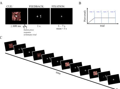
responses associated with each cue, the participant was told that, most of the time, the fractal would have a white circle at its center (normal contingency, or normal, trials) and they should respond according to the associations they had just seen. Participants were also told that occasionally the fractal cue would have a white triangle at its center instead of the circle (reversed contingency, or reversal, trials). On these trials, participants were instructed to respond to the cue using the opposite hand. For example, if the normal response to the fractal (with the circle in the center) was a right thumb button press, a triangle in the center would instead cue a reversal trial and thus, a left thumb button press.

Figure 2.1. Task design. A) Single-trial schematic. B) Graphic depicting temporal evolution of reversal trial probability. C) Sample sequence of events.

After finishing the experiment, all participants completed a battery of questionnaires designed to assess the effect of individual differences on the behavioral and neural responses to the task. The results of these analyses will be discussed in a separate manuscript.

Error analysis. Two types of errors are possible on reversal trials: an error of commission, in which the response is consistent with that fractal’s associated response in normal contingency trials, or an error of omission, in which the participant failed to enter any response during the allotted time. Because participants rarely made this second type of error, all incorrect trials were binned together for subsequent analysis. Errors on reversal trials, therefore, serve as our index of inhibitory control. Moreover, since there were no behavioral differences in performance by fractal identity (normal contingency performance x fractal identity ANOVA, p > 0.05), trials were grouped by condition for all subsequent behavioral and neural analyses. (A subsequent, post hoc analysis revealed no significant effect of fractal identity on neural response to either normal contingency or reversal cues.) These and other behavioral analyses were done using the Statistics Toolbox in MATLAB (Version 8.0.0.783, The MathWorks, Inc., Natick, Massachusetts).

T1-weighted structural images (TR = 1500 ms; TE = 3.05 ms; flip angle = 10o_{; voxel resolution = 1} mm3; single-shot, ascending acquisition) were also collected for each of the participants. These images were coregistered with the their respective EPI images to assist with the anatomical localization of the functional activations.

fMRI data preprocessing and statistical analysis. Imaging data analysis was performed using SPM5 (Wellcome Department of Imaging Neuroscience, Institute of Neurology, London, UK). Preprocessing of functional data consisted of correction for slice-time acquisition, motion correction and realignment to the mean image, spatial normalization to the Montreal Neurological Institute EPI template, and spatial smoothing using a Gaussian kernel with a full-width-half-maximum at 8 mm. Intensity filtering and high-pass temporal filtering (using a filter width of 128 s) were also applied to the data. All images were visualized using MRIcron software (http://www.sph.sc.edu/comd/rorden/mricron/).

To test for linear effects over time, we specified first-level contrasts separately for both normal contingency and reversal trials of the form [-0.75 -0.25 0.25 0.75] to test for linear increases in response and [0.75 0.25 -0.25 -0.75] to test for linear decreases in response over the four runs.

In order to address directly effects of performance on neural response for the two trial types, we estimated Model 2 with the following regressors of interest: (1) an indicator function for normal contingency trials where the correct response was entered (NormalCorrect, or NC), (2) an indicator for incorrect normal contingency trials (NormalIncorrect, or NI), (3) an indicator for correct reversal trials (ReversalCorrect, or RC), and (4) an indicator for incorrect reversal trials (ReversalIncorrect, or RI). All events were modeled with a duration of 0 s. Note that, as in the behavioral analysis, incorrect reversal trials were primarily errors of commission. The following first-level contrasts were computed for each individual: [NC - NI], [NI - NC], [RC-RI], [RI - RC], [NC - NI - RC + RI], [RC - RI - NC + NI], and [NC - NI + RC - RI]. (The final contrast identifies regions involved in processing correct responses relative to incorrect ones, while controlling for incorrect reversal responses, which were hypothesized to be similar to correct normal contingency responses.)

Results

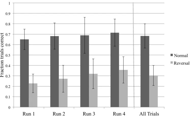
Behavioral results. Across all trials, participants responded with significantly greater accuracy on normal contingency trials (mean fraction correct = 0.68 ± 0.12) compared to reversal trials (mean fraction correct = 0.31 ± 0.096; t23 = 12.4, p < 0.001). Incorrect responses in reversal trials were primarily the button presses typically associated with the fractal cue (i.e., in normal contingency trials; mean fraction correct = 0.74 ± 0.14) rather than errors of omission. Since trials were also classified as incorrect if responses were entered after 600 ms (i.e., the subject received negative feedback at the end of the trial), we examined the accuracy of the button presses entered after the 600 ms period. For both trial types, performance was improved slightly for responses entered during the requisite window (normal: mean fraction correct = 0.80 ± 0.111; reversal: mean fraction correct = 0.56 ± 0.21), indicating that a longer response window would have improved accuracy.

Figure 2.2. Behavioral performance by condition across time. Rightmost panel shows performance averaged across all four runs.

A post hoc examination verified a significant linear trend over time for both normal trial (t23 = 2.78, p < 0.05) and reversal trial accuracy (t1,23 = 4.62, p < 0.001).

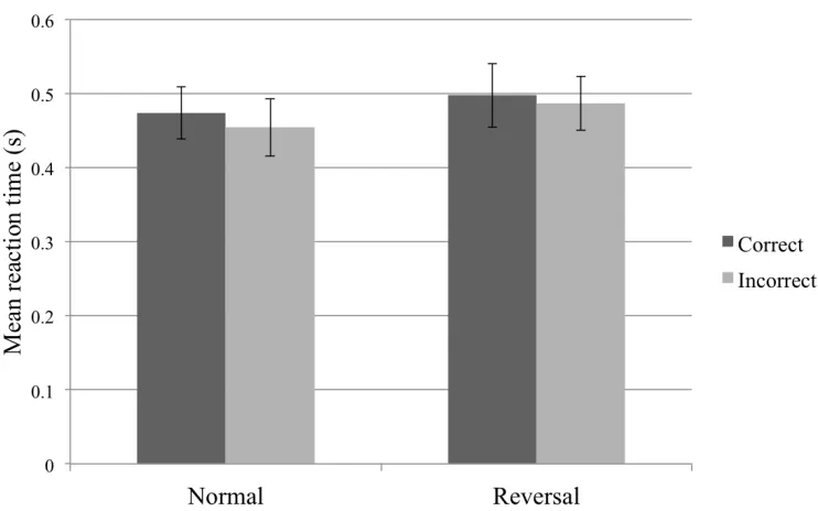
Figure 2.3. Reaction time by performance across conditions.

Figure 2.3 illustrates the reaction times over all trials for correct and incorrect trials in both conditions; values are listed in Table 2.1.

Performance

Correct Incorrect

Condition Normal 0.474 ± 0.035 0.454 ± 0.039

Reversal 0.497 ± 0.043 0.487 ± 0.037

Table 2.1. Mean reaction time by condition and performance. Mean (s) ± standard deviation.

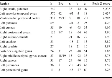
Region k BA x y z Peak Z score

Right insula, putamen 740 33 -12 -6 5.23*

Left superior temporal gyrus 570 42 -63 -3 18 5.03* Ventromedial prefrontal cortex 337 25/11 3 18 -12 4.79*

Left putamen 69 -24 -3 -9 4.26

Left cuneus 35 19 -6 -93 33 4.09

Right postcentral gyrus 125 5/7 18 -54 63 3.90

Right anterior caudate 23 21 36 -3 3.90

Left caudate 31 -18 21 15 3.89

Right caudate 27 18 21 15 3.87

Posterior cingulate gyrus 24 31 -9 -18 51 3.83

Right middle occipital gyrus, cuneus 33 18/19 15 -93 33 3.78

Right cuneus 31 17 24 -90 15 3.76

Left precuneus 36 5 -18 -45 63 3.59

Left postcentral gyrus 11 3 -45 -27 60 3.28

Table 2.2. Regions showing greater response for normal contingency compared to reversal trials. All results are reported at p < 0.001, uncorrected, with cluster extent ≥ 10 voxels.

* Whole-brain corrected for multiple comparisons (p < 0.05) at the cluster level (minimum cluster size = 194 voxels).

k = cluster size. Coordinates reported in MNI space.

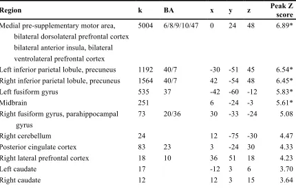
In contrast, stronger response in reversal trials was observed in a large cluster encompassing medial preSMA, bilateral ventrolateral, right insular, and left insular cortices (including left vlPFC). Other regions demonstrating higher neural response for reversal compared to normal contingency trials included bilateral inferior parietal lobule, bilateral precuneus, left fusiform gyrus, and midbrain (p < 0.05, WBC; Table 2.3).

Region k BA x y z Peak Z _score

Medial pre-supplementary motor area, 5004 6/8/9/10/47 0 24 48 6.89* bilateral dorsolateral prefrontal cortex

bilateral anterior insula, bilateral ventrolateral prefrontal cortex

Left inferior parietal lobule, precuneus 1192 40/7 -30 -51 45 6.54* Right inferior parietal lobule, precuneus 1564 40/7 42 -54 48 6.45*

Left fusiform gyrus 535 37 -42 -60 -12 5.83*

Midbrain 251 6 -24 -3 5.61*

Right fusiform gyrus, parahippocampal 73 20/36 30 -33 -24 5.08 gyrus

Right cerebellum 24 12 -75 -30 4.47

Posterior cingulate cortex 83 23 3 -24 30 4.33

Right lateral prefrontal cortex 18 10 36 51 18 4.23

Left caudate 17 -12 3 6 3.70

Right caudate 12 12 3 15 3.64

Table 2.3. Regions showing greater response for reversal compared to normal contingency trials. All results are reported at p < 0.001, uncorrected, with cluster extent ≥ 10 voxels.

* Whole-brain corrected for multiple comparisons (p < 0.05) at the cluster level (minimum cluster size = 194 voxels).

k = cluster size. Coordinates reported in MNI space.

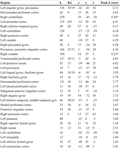
Figure 2.5. Voxels showing linear effects of time for each condition. A) Regions showing a positive linear effect in normal contingency trials. B) Regions showing a negative linear effect in reversal trials. The warm color scale reflects linear increases in response over time, while the cool color scale reflects linear decreases in response over time.

Region k BA x y z Peak Z score

Left angular gyrus, precuneus 156 39/19 -42 -81 36 4.73

Dorsomedial prefrontal cortex 42 9 15 36 33 4.63

Right cerebellum 220 39 -45 -36 4.54*

Left premotor cortex 155 6/8 -12 30 63 4.41

Right inferior temporal gyrus 30 20 57 -6 -27 4.37

Left cerebellum 128 -27 -72 -39 4.34

Right premotor cortex 29 8 27 42 51 4.30

Left caudate 68 -18 27 9 4.29

Right precentral gyrus 50 4 15 -24 54 4.28

Precuneus, posterior cingulate cortex 166 23/31 3 -54 24 4.36

Right caudate 194 24 33 3 4.22*

Ventromedial prefrontal cortex 127 10/11 -3 42 -6 4.05

Left posterior insula 55 13 -39 -48 21 4.02

Left precuneus 14 7 -15 -57 39 3.96

Left lingual gyrus, fusiform gyrus 44 18/19 -6 -81 -6 3.93

Right fusiform gyrus 19 18 27 -72 -12 3.79

Dorsomedial prefrontal cortex 121 10 -12 60 24 3.77

Left lateral prefrontal cortex 11 10 -30 57 6 3.76

Subgenual anterior cingulate cortex 12 25 3 15 -18 3.74

Right angular gyrus 19 39 54 -72 36 3.72

Left inferior temporal, middle temporal gyri 46 20/21 -57 -3 -27 3.69

Medial prefrontal cortex 33 10 -6 54 12 3.67

Posterior cingulate cortex 19 30 -21 -57 9 3.66

Right premotor cortex 13 6 12 27 63 3.66

Left putamen 40 -21 6 -3 3.64

Right superior frontal gyrus 29 10 21 51 33 3.58

Right insula 15 13 51 -15 9 3.51

Left cerebellum 16 -42 -51 -30 3.46

Left amygdala 12 -18 -6 -18 3.46

Left inferior frontal gyrus 16 47 -48 45 -3 3.45

Left extrastriate cortex 18 18 -12 -99 3 3.42

Table 2.4. Regions showing positive linear effects of time in normal contingency trials

All results are reported at p < 0.001, uncorrected, with cluster extent ≥ 10 voxels. * Whole-brain corrected for multiple comparisons (p < 0.05) at the cluster level (minimum cluster size = 174 voxels).

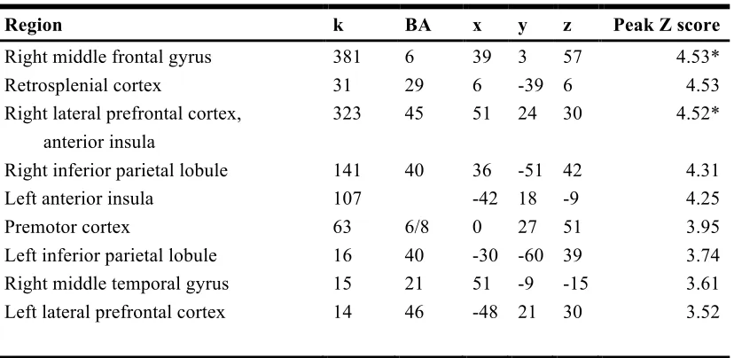
In contrast, only a negative linear effect was evident in reversal trials, with premotor cortex and right lateral PFC extending into insula showing particularly strong decreases in neural response over time (p < 0.05, WBC; Figure 2.5B, Table 2.5).

Region k BA x y z Peak Z score

Right middle frontal gyrus 381 6 39 3 57 4.53*

Retrosplenial cortex 31 29 6 -39 6 4.53

Right lateral prefrontal cortex, 323 45 51 24 30 4.52* anterior insula

Right inferior parietal lobule 141 40 36 -51 42 4.31

Left anterior insula 107 -42 18 -9 4.25

Premotor cortex 63 6/8 0 27 51 3.95

Left inferior parietal lobule 16 40 -30 -60 39 3.74

Right middle temporal gyrus 15 21 51 -9 -15 3.61

Left lateral prefrontal cortex 14 46 -48 21 30 3.52

Table 2.5. Regions showing negative linear effects of time in reversal trials. All results are reported at p < 0.001, uncorrected, with cluster extent ≥ 10 voxels.

* Whole-brain corrected for multiple comparisons (p < 0.05) at the cluster level (minimum cluster size = 173 voxels).

k = cluster size. Coordinates reported in MNI space.

Direct contrasts between normal and reversal for both the positive linear and negative linear effects confirmed that changes over time were unique to each condition (all p < 0.01, uncorrected).

Contrast Region k BA x y z Peak Z score

NC - NI

Posterior cingulate cortex, striatum, 3768 31 3 -42 36 5.28* ventromedial prefrontal cortex

Left premotor cortex 261 8/6 -18 30 54 5.27

Right extrastriate cortex, cuneus, 293 18 27 -96 9 5.17* lingual gyrus

Left primary visual cortex 275 17 -21 -96 6 4.55*

Left precuneus, angular gyrus 62 39 -36 -66 30 4.32

Right superior temporal gyrus 36 22 57 -9 -3 4.30

Right premotor cortex 280 8/6 24 24 57 4.24*

Right inferior temporal gyrus 67 20 60 -9 -24 4.10

Left hippocampus 27 -30 -33 -3 4.00

Left superior temporal gyrus 18 22 -54 -9 -3 3.98

Right angular gyrus 32 39 48 -72 36 3.84

Left middle temporal gyrus 16 41 -54 -45 -9 3.59

Dorsomedial cingulate cortex 13 32 3 -9 30 3.39

NI - NC

Left anterior insula 229 -33 21 9 5.39

Right anterior insula 190 36 18 9 4.64

Medial premotor cortex, right

supplementary motor cortex 299 32/6 6 15 42 4.40*

Right supramarginal gyrus 75 40 63 -45 27 4.31

Right dorsolateral prefrontal cortex 46 9 42 6 33 4.15 Left dorsolateral prefrontal cortex 42 9 -42 15 33 4.00

Left superior parietal lobule 29 7 -27 -60 42 3.75

Precuneus 23 31 -9 -69 18 3.64

Left supplementary motor cortex 17 6 -9 -9 72 3.64

Right parahippocampal gyrus 10 30 18 -54 0 3.37

Left parahippocampal gyrus 11 30 -18 -60 0 3.33

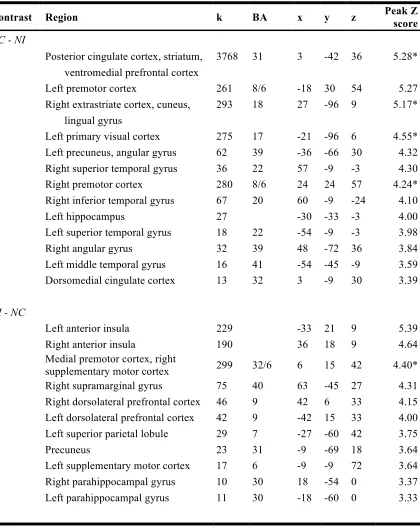
Table 2.6. Regions showing differential effects for correct and incorrect normal trials. All results are reported at p < 0.001, uncorrected, with cluster extent ≥ 10 voxels.

* Whole-brain corrected for multiple comparisons (p < 0.05) at the cluster level (minimum cluster size = 257 voxels).

We examined our third hypothesis by testing specifically for the involvement of cognitive control regions in trials for correct reversal responses. Significant effects for reversal trials were only found for correct > incorrect trials; correct responses in these trials were associated with activity in right supplementary motor areas (p < 0.05, WBC) and left vlPFC (p < 0.05, SVC), among others (Figure 2.7, Table 2.7).

Contrast Region k BA x y z Peak Z score

RC - RI

Right supplementary motor cortex 333 6/8 21 24 63 4.72* Left ventrolateral prefrontal cortex 127 11 -42 42 -9 4.64

Right angular gyrus 138 7/40 51 -63 51 4.49

Left supplementary motor cortex 121 6 -30 18 60 4.46

Left ventral striatum 98 -12 6 -9 4.42

Left angular gyrus 50 7 -39 -72 45 4.08

Left anterior insula 28 -36 15 -6 3.88

Anterior cingular gyrus 36 32 3 39 -3 3.87

Right anterior insula 57 45 30 -9 3.74

Medial prefrontal cortex 141 10 0 57 21 3.56

Left fusiform gyrus 26 20 -51 -39 -27 3.46

RI - RC

No significant voxels

Table 2.7. Regions showing differential effects for correct and incorrect reversal trials. All results are reported at p < 0.001, uncorrected, with cluster extent ≥ 10 voxels.

* Whole-brain corrected for multiple comparisons (p < 0.05) at the cluster level (minimum cluster size = 205 voxels).

k = cluster size. Coordinates reported in MNI space.

controlling for incorrect responses on reversal trials, since those responses required the same motor action as the correct normal contingency response. Stronger BOLD response was observed in bilateral premotor areas, PCC, and ventral striatum extending into medial PFC (p < 0.05, WBC; Figure S2.3, Table S2.3).

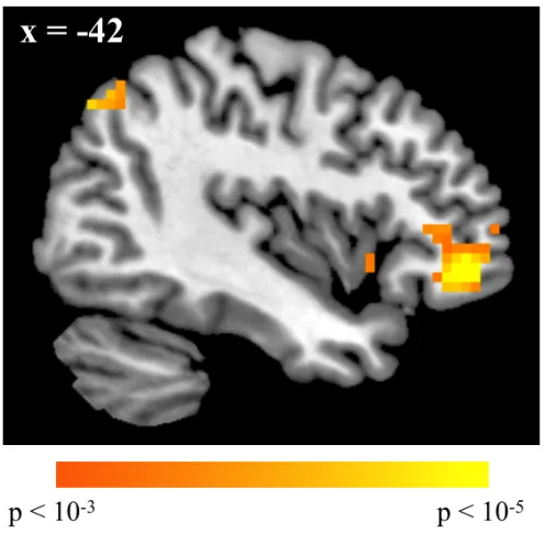
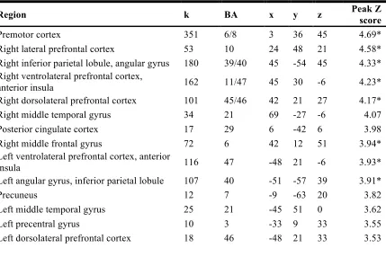
Finally, to interrogate our fourth hypothesis, we examined linear changes in response – particularly in infrequent (i.e., reversal) trials – over time with respect to performance. For correct reversal trials, we saw decreases in response over time in a variety of regions, including medial preSMA, left and right vlPFC, right lateral PFC, and right inferior parietal lobule (p < 0.05, WBC; Figure 2.8, Table 2.8). No regions showed increase response over time for correct reversal trials. All other results showing linear changes in neural response as a function of response accuracy are described in Supplementary Materials (incorrect reversal trials: Figure S2.4 and Table S2.4 correct normal trials: Figure S2.5 and Table S2.5; incorrect normal contingency trials: Figure S2.6 and Table S2.6).

Region k BA x y z Peak Z score

Premotor cortex 351 6/8 3 36 45 4.69*

Right lateral prefrontal cortex 53 10 24 48 21 4.58*

Right inferior parietal lobule, angular gyrus 180 39/40 45 -54 45 4.33* Right ventrolateral prefrontal cortex,

anterior insula 162 11/47 45 30 -6 4.23*

Right dorsolateral prefrontal cortex 101 45/46 42 21 27 4.17*

Right middle temporal gyrus 34 21 69 -27 -6 4.07

Posterior cingulate cortex 17 29 6 -42 6 3.98

Right middle frontal gyrus 72 6 42 12 51 3.94*

Left ventrolateral prefrontal cortex, anterior

insula 116 47 -48 21 -6 3.93*

Left angular gyrus, inferior parietal lobule 107 40 -51 -57 39 3.91*

Precuneus 12 7 -9 -63 20 3.82

Left middle temporal gyrus 25 21 -45 51 0 3.62

Left precentral gyrus 10 3 -33 9 33 3.55

Left dorsolateral prefrontal cortex 18 46 -48 21 33 3.53

Table 2.8. Regions showing negative linear effects of time in correct reversal trials. All results are reported at p < 0.001, uncorrected, with cluster extent ≥ 10 voxels.

* Whole-brain corrected for multiple comparisons (p < 0.05) at the cluster level (minimum cluster size = 42 voxels).

k = cluster size. Coordinates reported in MNI space.

Discussion

were further modulated by performance, where an effect of automaticity was observed in regions including right vlPFC – an area thought to be necessary for cognitive control12 – only in trials where response inhibition was implemented successfully. These findings replicate and extend previous work identifying neural regions involved in cognitive control and response automaticity, and provide additional support for the theory that automaticity in cognitive control is associated with neural efficiency.

Learned automaticity in neural response to reversal trials was evidenced by a decrease in BOLD response over time in premotor cortex and right vlPFC extending into insula; no regions showed a linear increase in signal over sessions. This effect was unique to reversal trials, since there were no common activations for temporal response patterns between normal and reversal trials. Moreover, as experience with cognitive control increased over time, correct responses were associated with reductions in neural response in several regions that have been linked to cognitive control, including medial preSMA122,137-139,157, right vlPFC (e.g., 21,98,114-122,126-129), right lateral PFC98,114, and right inferior parietal cortex15,130. These data are in line with the work of Chiu and others (2012), who demonstrated that the magnitude of motor evoked potentials decreases as performance improves in the ‘no-go’ trials of a typical go/no-go paradigm155, and extend their work to fMRI, which offers more precise localization of effects. Reductions in neural response in association with training and improvement in individual performance may be indicative of increased efficiency, especially in cognitive tasks (e.g., 164,173-176). Together, such data imply that the cognitive control performance enhancements associated with increased automaticity may be mediated by increased neural efficiency.

time was relatively unchanged, and changes were only evident in slight reductions in standard deviation, particularly between the first and second half of the experiment. Even as improvements in accuracy indicated learning over time, the task remained difficult – the highest average performance (in run 4) for normal contingency was 71.4% and 35.7% for reversal trials – and required vigilance for the duration of the experiment.

Several additional issues should be considered in the interpretation of these findings. First, with respect to the role of vlPFC in response inhibition, recent data have suggested that right vlPFC activation in go/no-go tasks may reflect a more general attentional salience detection mechanism148,177. Neither our experiment nor any of the others cited here can fully rule out this interpretation, since response inhibition tasks typically make use of “oddball” style designs, where the stimuli requiring control are far less frequent than the other stimuli, enhancing their novelty or salience. However, it is worth noting that lesions to frontal areas, including the vlPFC, critically affect performance on the Wisconsin Card Sorting Test, a neuropsychological battery that, like many other task switching paradigms, measures behavioral flexibility in response to changing reinforcement schedules178,179_.

Another source of individual variability was task in strategy180 _{– for example, whether to strive for} speed or accuracy; such differences manifest in both brain and behavior and can impact interpretation. While we cannot know whether individuals were more motivated by speed or accuracy strategies, we can assume that strategic bias was minimized by the experimental design, which provided both speed and accuracy incentives. We limited the response period to 600 ms, since a short response period has also been shown to increase the likelihood of observing response inhibition181 and is less likely than a long window to induce bias toward accuracy, since time for the evolution of cognitive processes is limited. We balanced any potential speed bias by providing motivationally salient feedback on each trial, a technique that has been shown to impact go/no-go learning both behaviorally and neurally in STN/VTA and vlPFC182. Indeed, our behavioral data indicate that we were able to mitigate any potential strategic bias; standard deviations were of comparable magnitude across normal and reversal trials, indicating that the speed incentive did not affect learning differentially during reversal trials. Moreover, when participants entered responses outside the 600 ms window on reversal trials, these responses were generally accurate, suggesting strong motivation to enter a correct response on each trial; additionally, post-task self-report suggested that participants were motivated by the feedback, and individuals were especially frustrated when they made errors of commission on reversal trials.

Figure S2.1. Voxels showing differences for normal contingency and reversal trials when controlling for performance.

Table S2.1. Regions activated for the contrast [NC - NI - RC + RI].

Region k BA x y z Peak Z score

Right superior temporal gyrus 114 42 63 -24 6 4.50

Right paracentral lobule 44 5 12 -36 57 4.44

Right subgenual cingulate cortex 25 25 15 30 -6 4.42

Right caudate 20 21 3 30 4.24

Subgenual cingulate cortex 17 25 -3 24 -15 4.21

Left posterior insula 31 13 -27 -36 18 4.16

Left caudate 20 -21 15 24 4.02

Right postcentral gyrus 25 5 21 -42 63 3.94

Ventromedial prefrontal cortex 65 11 -3 45 -12 3.93

Right posterior insula 19 13 27 -27 24 3.93

Left hippocampus 15 -27 -27 -3 3.68

Right extrastriate cortex 19 18 24 -96 -3 3.45

Table S2.2. Regions activated for the contrast [RC - RI - NC + NI].

Region k BA x y z Peak Z score

Left insula 276 13 -33 21 6 5.30*

Premotor cortex 266 6/8 6 15 63 5.07*

Right insula 313 13 36 24 -3 4.54*

Left ventrolateral prefrontal cortex 19 11 -42 42 -6 3.91

Left precentral gyrus 15 9 -57 12 42 3.88

Left superior parietal lobule 29 7 -30 -60 45 3.78

Right supramarginal gyrus 22 40 63 -57 39 3.57

Left dorsolateral prefrontal cortex 29 46 -48 21 24 3.49

All results are reported at p < 0.001, uncorrected, with cluster extent ≥ 10 voxels.

* Whole-brain corrected for multiple comparisons (p < 0.05) at the cluster level (minimum cluster size = 183 voxels).

Table S2.3. Regions activated for the contrast [NC - NI + RC + RI].

Region k BA x y z Peak Z score

Left premotor cortex 394 6/8 -24 21 66 5.15*

Right premotor cortex 372 6/8 21 24 63 5.05*

Posterior cingulate cortex 310 31 -3 -48 33 5.07*

Ventral striatum, medial prefrontal cortex 1547 32/9/10 -15 9 -9 4.68*

Right visual cortex 126 18/17 24 -93 3 4.63

Right inferior parietal lobule 196 7/40 57 -63 45 4.49

Left inferior parietal lobule 83 7/39/40 -39 -72 45 4.28

Right inferior temporal gyrus 60 21 57 -9 -21 4.12

Left cuneus 45 17 -18 -93 0 4.09

Mediodorsal cingulate gyrus 94 24 -12 -12 33 3.96

Left inferior temporal gyrus 106 20/21 -60 -36 -18 3.92

Right cerebellum 10 42 -63 -42 3.90

Left inferior frontal gyrus 13 47 -45 36 6 3.76

Left ventrolateral prefrontal cortex 59 11 -39 45 -6 3.59

Left lateral prefrontal cortex 13 10 -33 54 9 3.41

All results are reported at p < 0.001, uncorrected, with cluster extent ≥ 10 voxels.

* Whole-brain corrected for multiple comparisons (p < 0.05) at the cluster level (minimum cluster size = 243 voxels).

Figure S2.4. Voxels showing linear effects of time for incorrect reversal trials.

Table S2.4. Regions exhibiting linear change in response over time for incorrect reversal trials.

Contrast Region k BA x y z Peak Z

score

Linear increase over runs

Right cerebellum 23 36 -42 -36 4.33

Right paracentral lobule 11 31 15 -24 54 4.17

Right extrastriate cortex 41 18 12 -102 15 3.84

Right cingulate gyrus 12 24 21 9 33 3.47

Linear decrease over runs

Left anterior insula 36 47 -42 18 -9 4.26

Right fusiform gyrus 11 37 51 -51 -21 3.68

Right superior temporal gyrus 11 22 51 -39 12 3.59

Right supramarginal gyrus 11 40 45 -51 36 3.42

Table S2.5. Regions exhibiting linear increase in response over time for correct normal contingency trials.

Region k BA x y z Peak Z score

Premotor cortex 471 6/9/10 -12 30 63 4.61*

Left angular gyrus, inferior parietal lobule 138 39 -42 -81 36 4.57*

Right cerebellum 217 39 -51 -45 4.51*

Frontal lobe (white matter) 107 24 21 27 4.45*

Left superior temporal gyrus 35 39 -39 -48 21 4.29

Right middle temporal gyrus 26 20/21 57 -6 -27 4.21

Right superior frontal gyrus 35 8 24 42 51 4.2

Left cerebellum 103 -24 -75 -36 4.05*

Left ventrolateral prefrontal cortex 52 47/11 -48 30 -3 4.02*

Left middle temporal gyrus 56 21 -60 -36 -3 3.91*

Right superior frontal gyrus 90 9/10 21 51 36 3.87*

Left lingual gyrus 32 18 -9 -81 -6 3.85

Posterior cingulate cortex 94 31 0 -57 18 3.83*

Frontal lobe (white matter) 10 -15 12 24 3.81

Right supplementary motor area 15 6 24 -21 54 3.73

Left supplementary motor area 11 6 -3 12 72 3.73

Left supramarginal gyrus 33 40 -63 -48 42 3.69

Left putamen 11 -21 3 12 3.65

Right angular gyrus 16 39 54 -72 36 3.63

Left hippocampus, parahippocampal gyrus 20 -21 -12 -15 3.61

Left precuneus 10 7 -18 -57 39 3.6

Right putamen 14 21 9 9 3.59

Ventromedial prefrontal cortex 82 10/11 3 42 -15 3.58*

Left superior frontal gyrus 12 8 -33 24 48 3.42

Left extrastriate cortex 17 18 -12 99 9 3.41

Left cerebellum 20 -39 -54 -30 3.37

All results are reported at p < 0.001, uncorrected, with cluster extent ≥ 10 voxels.

* Whole-brain corrected for multiple comparisons (p < 0.05) at the cluster level (minimum cluster size = 45 voxels).

Table S2.6. Regions exhibiting linear increase in response over time for incorrect normal contingency trials.

Region k BA x y z Peak Z score

Right cerebellum 39 39 -45 -36 4.78

Left lingual gyrus 11 30 -15 -42 0 4.72

Left cerebellum 42 -45 -51 -33 4.54

Posterior cingulate cortex 137 23/31 0 39 33 4.41*

Left cerebellum 25 -27 -72 -39 3.93

Left middle temporal gyrus 18 21 -42 0 -30 3.86

Left precuneus 33 19 -42 -78 36 3.77

Pons 10 3 -27 -39 3.75

Right supplementary motor area 18 6 21 -24 54 3.62

Posterior cingulate cortex 11 30 -18 -54 9 3.52

Left cerebellum 19 -18 -63 -33 3.47

All results are reported at p < 0.001, uncorrected, with cluster extent ≥ 10 voxels.

* Whole-brain corrected for multiple comparisons (p < 0.05) at the cluster level (minimum cluster size = 45 voxels).

C h a p t e r 3

INTRA-PREFRONTOCORTICAL CONNECTIVITY IN TEMPORAL DISCOUNTINGÛ

There is widespread interest in identifying computational and neurobiological mechanisms that influence the ability to choose long-term benefits over more proximal and readily available rewards in domains such as dietary and economic choice. We present the results of a human fMRI study that examines how neural activity relates to observed individual differences in the discounting of future rewards during a monetary ITC task. We found that portions of left dlPFC, in BA 9 and 46, were more active in trials where subjects chose delayed rewards, after controlling for the subjective value of those rewards. We also found that the connectivity from dlPFC-BA46 to a region of vmPFC widely associated with the computational of stimulus values, increased at the time of choice, and especially during trials in which subjects chose delayed rewards. Finally, we found that estimates of effective connectivity between these two regions played a critical role in predicting out-of-sample between-subject differences in discount rates. Together with previous findings in dietary choice, these results suggest that a common set of computational and neurobiological mechanisms facilitate virtuous choice in both settings.

Introduction

Impaired self-control is thought to play a critical role in sub-optimal decision-making, and in conditions like addiction and obesity28,97. As a result, there is a widespread, on-going effort to characterize the computational and neurobiological mechanisms underlying self-control. Two types of paradigms have been widely used in behavioral neuroscience to examine these mechanisms. First are tasks involving intertemporal decisions between rewards, often money, in which subjects choose between sooner-smaller amounts and later-larger ones70,74,76,77,79-81,97,183,184_{. Second, are tasks}

involving dietary choices, in which subjects make choices between foods that vary in their tastiness and healthiness88,89,185.

In previous work investigating dietary self-control, we found important commonalities and differences between successful and unsuccessful dieters88_{. Behaviorally, the two groups differed on} the relative weight that they placed on the health and taste attributes of foods in making their decisions (with successful dieters weighting both health and taste, and unsuccessful dieters weighting only taste). Neurally, the vmPFC encoded the value of foods at the time of choice equally for both groups. The critical difference had to do with the role of left dlPFC. In successful dieters, dlPFC came on-line and exhibited increased effective connectivity with vmPFC during choices that required self-control (e.g., refusing to eat tasty, but unhealthy, candy). In contrast, unsuccessful dieters did not exhibit this pattern of connectivity. Furthermore, in a subsequent study we found that non-dieting participants behaved like successful dieters if they were given an exogenous reminder to pay attention to health information, and that the reminder activated the same dlPFC-vmPFC networks that successful dieters activated on their own89.

the vmPFC will assign values to options that are not consistent with the long-term, goal-relevant (e.g., proper nutrition) rewards they generate.

An important open question is whether this pattern of interregional neural activity is also involved in other decision domains, such as those involving intertemporal monetary tradeoffs. This question is important because comparing the mechanisms at work in different decision contexts is a critical step in identifying common mechanisms that facilitate self-control. Theoretically, these circuits should also influence the degree of discounting for delayed rewards in the case of ITC, as long as dlPFC modulation of vmPFC can lead to an increased (or decreased) weighting for delayed rewards.

Here we address this open question by testing the following three hypotheses. First, we hypothesized that the same sub-regions of left dlPFC that are more active during self-control in dietary choice would also be more active in ITC when the subjects choose the larger-delayed payment over the money available today, after controlling for their value difference. Note that it is crucial to control for the value difference, because if the subjective value of the delayed reward is large enough, the decision to wait becomes trivial. Second, we hypothesized that effective connectivity from left dlPFC to vmPFC would be stronger during trials in which subjects choose larger-delayed rewards (again controlling for subjective value), which is consistent with the idea that dlPFC can modulate the value signals in vmPFC so that they place more weight on the value of delayed payouts. Third, we hypothesized that the levels of activation in dlPFC, as well as its effective connectivity to vmPFC, would help to explain differences in discount rates across subjects.

wide variety of decision contexts187-196_{, including decisions involving intertemporal} tradeoffs74,76,88,89,197. Second, previous studies have associated responses in left dlPFC with choosing to wait for delayed monetary rewards using transcranial magnetic stimulation (TMS) and fMRI79,82_. In particular, Figner et al. (2010) showed that temporarily reducing activity in left dlPFC using TMS results in subjects making more impatient choices, thus, establishing a causal role for this region in temporal discounting82. Third, recent studies have found that resting-state connectivity in networks including left dlPFC was correlated with discount rates198,199.

Despite the attractiveness of the theory, and the body of consistent evidence, critical questions remain open. In particular, none of the previous studies have examined the effective connectivity between dlPFC and vmPFC during ITCs, nor can they establish that the dlPFC influences discount rates through a mechanism that involves the modulation of the stimulus values computed in vmPFC, or that the effective connectivity runs from dlPFC to vmPFC, and not the other way around. Here we are able to address these questions by estimating dynamic causal models200_{, and} using their estimates to explain and predict differences in discount rates across individuals.

Materials and methods

ITC task. On every trial, subjects chose between getting $25 at the end of the experiment, and getting an equal or larger amount at a later date. The later offers ranged from $25 to $54, with a delay from 7 to 200 days. Subjects made 216 decisions. The unique combinations of amount and delay used are shown in Table S3.1. All subjects saw the same set of options, although in different random orders. Each option was shown twice. Note that presenting all subjects with the same options was necessary to subsequently test how neural activity relates to discount rates. Although beneficial for the hypotheses tested in previous studies74,77,201, tailoring the choice sets around the indifference points of each subject would create a confound when examining how individual differences in neural activity relate to discount rates, since less patient subjects would be shown delayed rewards with higher monetary values.

Figure 3.1. Task design and behavioral data. A) Example display screens and timing parameters. B) Choice curve displaying the probability of choosing the larger, delayed reward. The y-axis shows the probability of selecting the future reward and the x-axis displays the stimulus value of the future reward. Error bars represent the standard error of the mean. C) Bar graph showing the distribution of discounting parameters.

All payments were made using prepaid debit cards given to the subjects at the end of the experiment. This allowed us to make the delayed payments available on the appropriate date, without requiring subjects to return to the lab.

delayed options using a hyperbolic discounting function, in which the value of $A with a delay of D days is given by

dSV = A/(1+kD),

where dSV denotes the discounted stimulus value. We also assumed that the probability of accepting the delayed option is given by the soft-max function

P(Yes) = (1+exp(b*(25 - dSV)))-1,

where b is a non-negative parameter that modulates the slope of the psychometric choice function. Note that in this formula the value of the constant reference option is $25.

fMRI data preprocessing. Imaging data were preprocessed using SPM8 (Wellcome Department of Imaging Neuroscience, Institute of Neurology, London, UK). Data were corrected for motion with realignment to the mean image, spatially normalized to the Montreal Neurological Institute EPI template, resampled to 3 mm3 voxels, and spatially smoothed using a Gaussian kernel (full-width-at-half-maximum = 8 mm). Data were also temporally filtered using a filter width of 128 s.

GLMs. We estimated two different mixed effect models of the BOLD responses, with AR(1). The models were designed to localize in our sample the areas of vmPFC and vStr that, as discussed in the introduction, have been repeatedly shown to correlate with stimulus values at the time of choice. The models are identical except for the specification of the value modulators.

The first model, GLM-1, had the following regressors of interest: 1) an indicator function beginning at the onset of each decision screen with duration equal to the reaction time for that trial, 2) the indicator function modulated by the subject specific value of each delayed offer (dSV), and 3) the indicator function modulated by the variable Accept (which equals 1 if the subject chooses the delayed outcome, and zero otherwise). The third regressor was orthogonalized with respect to the second one in order to assign any shared variance between them to the dSV regressor. The model also included session dummies, linear time trends, and head movements as regressors of no interest.