BIROn - Birkbeck Institutional Research Online
Paterson, Maura B. and Stinson, D. (2016) Combinatorial characterizations
of algebraic manipulation detection codes involving generalized difference
families. Discrete Mathematics 339 (12), pp. 2891-2906. ISSN 0012-365X.
Downloaded from:
Usage Guidelines:
Please refer to usage guidelines at or alternatively
Combinatorial Characterizations of Algebraic Manipulation
Detection Codes Involving Generalized Difference Families
Maura B. Paterson1 and Douglas R. Stinson∗2
1Department of Economics, Mathematics and Statistics, Birkbeck, University of London,
Malet Street, London WC1E 7HX, UK
2David R. Cheriton School of Computer Science, University of Waterloo, Waterloo,
Ontario, N2L 3G1, Canada
March 8, 2016
Abstract
This paper provides a mathematical analysis of optimal algebraic manipulation detection (AMD) codes. We prove several lower bounds on the success probability of an adversary and we then give some combinatorial characterizations of AMD codes that meet the bounds with equality. These characterizations involve various types of generalized difference families. Con-structing these difference families is an interesting problem in its own right.
1
Introduction
Algebraic manipulation detection (AMD) codes were defined in 2008 by Cramer et al. [3, 4] as a generalization and abstraction of techniques that were previously used in the study of robust secret sharing schemes [14, 15, 17]. AMD codes are studied further in [1, 5, 6]. Several interesting and useful applications of these structures are described in these papers, including applications to robust fuzzy extractors, secure multiparty computation, non-malleable codes, etc. Various construction methods for AMD codes are also presented in these papers.
We begin by providing some motivating examples as well as some historical context from the point of view of authentication codes. AMD codes can be considered as a variation of the classical
unconditionally secure authentication codes [16], which we will refer to as A-codes for short. An
A-code has the form (S,T,K,E) whereSis a set of plaintextsources,T is a set oftags,Kis a set of
keysandEis a set ofencoding functions. For eachK ∈ K, there is a (possibly randomized) encoding function EK :S → T. A secret key K ∈ K is chosen randomly. Later a source s ∈ S is selected
and the tagt =EK(s) is computed. The tag t is authenticated by verifying that t=EK(s); this
can be done only with knowledge of the keyK. Having seen a valid pair (s, t), an active adversary may create a bogus pair (s0, t0) (where s0 6=s), hoping that it will be accepted as authentic (this process is calledsubstitution). The adversary is trying to maximize thesuccess probability of such an attack. One main objective is to design A-codes that will minimize the success probability of the adversary.
∗
Example 1.1. Let pbe prime and defineS =T =Zp. DefineK=Zp×Zp. For everyK = (c, d)∈ K, define the function EK by the rule s 7→ cs+dmodp for all s ∈ Zp. (That is, the encoding
functions consist of all linear functions from Zp toZp.) Any observed source-tag pair(s, t) is valid
under exactly p of the p2 keys. Then, any substitution (s0, t0) (s0 6=s) is valid under exactly 1 of the p “possible” keys. Therefore, the adversary’s success probability is 1/p.
There are two types of AMD codes. The first type is a weak AMD code. Here there is no key, so there is only one encoding functionE. Further, the tag is an element of a finite additive abelian group, sayG. The adversary is required to commit to a specific substitution of the formg7→g+ ∆, where ∆ ∈ G \ {0} is fixed. Later, a source s ∈S is chosen randomly and encoded to g = E(s). Then g is replaced by g0 = g+ ∆. The adversary wins if g0 =E(s0) for some s6=s0. Again, the objective in designing such a code is to minimize the adversary’s success probability.
Example 1.2. Let S = {1,2,3,4,5} and let G = Z21. The encoding function E is defined by
E(1) = 3, E(2) = 6,E(3) = 12, E(4) = 7 andE(5) = 14. It turns out that the adversary’s success probability is 1/5, independent of his choice of ∆ 6= 0. This follows because {3,6,12,7,14} is a difference set inZ21 (for the definition of difference set, see Section 2).
The second type of AMD code is a strong AMD code. It is basically the same as a weak AMD code, except that the adversary is given the source (but not the encoded version of the source) before choosing ∆.
Example 1.3. This example is based on Example 2.7. Let S = {1,2,3,4} and let G = Z7.
The encoding function E is defined by E(1) = 1, E(2) = 2, E(3) = 4 and E(4) ∈R {0,3,5,6}
(the notation “∈R” denotes that the given encoding is to be chosen uniformly at random from the given set). If the source s = 1,2 or 3, then the adversary succeeds with probability 1 by choosing ∆ such that E(s) + ∆ = E(s0) for some s0 6= s. However, if the source s = 4, it can be verified that the adversary’s success probability is 1/2. To see this, observe for any ∆6= 0 that
E(4) + ∆∈ {E(1), E(2), E(3)} for precisely two of the four possible values of E(4).
1.1 Notation
In this section, we present relevant notation that we will use in the rest of the paper.
• There is a setS of plaintext messages which is termed thesource space, where|S|=m. There will be a probability distribution on S, which is assumed to be public. We will normally assumePr[s] = 1/mfor all s∈ S, so we have equiprobable sources.
• The encoded message space(or more simply, message space) is a setG, where|G|=n(note:
G will usually be an additive abelian group with identity 0).
• For every sources∈ S, let A(s)⊆ G denote the set of valid encodings of s. We require that
A(s)∩A(s0) =∅ if s6=s0; this ensures that any message can be correctly decoded. Denote
A={A(s) :s∈ S}.
• Letas=|A(s)|for anys∈ S. Define
G0= [
s∈S
and denote
a=X
s∈S
as.
Ifas is constant, sayk, then the code is k-uniform. In this case, a=km.
• E :S → G is a (possibly randomized) encoding function that maps a source s∈ S to some
g∈A(s) according to a certain probability distribution defined onA(s):
Pr[E(s) =g] =Pr[g|s].
The encoding functionE, as well as the probability distributions Pr[E(s) =g], are assumed to be public. Observe that, for equiprobable sources, the induced probability distribution on
G0 is given by
Pr[g] = 1
m×Pr[E(s) =g]
for all s∈ S and allg∈A(s).
• Formally, we can define the AMD code as a 4-tuple (S,G,A, E).
• If Pr[E(s) =g] = 1/as for every s∈ S and every g ∈ A(s), then the code has equiprobable
encoding. Such a code can be denoted as a 3-tuple (S,G,A). In a code with equiprobable sources and equiprobable encoding, we have
Pr[g] = 1
asm
for all s∈ S and allg∈A(s).
• A k-uniform code that has equiprobable sources and equiprobable encoding is said to be
k-regular. In a k-regular code, we have
Pr[g] = 1
km
for all g∈ G0.
• A 1-regular code is said to be deterministic because the source uniquely determines the encoding. In a deterministic code with equiprobable sources, we have
Pr[g] = 1
m
for all g∈ G0.
1.2 Formal Definitions of Weak and Strong AMD Codes
Definition 1.1 (Weak AMD code). Suppose (S,G,A, E) is an AMD code.
1. The value ∆∈ G \ {0} is chosen according to the adversary’s strategy.
2. The source s∈ S is chosen uniformly at random by the encoder (i.e., we have equiprobable sources).
3. The source is encoded into g∈A(s) using the encoding functionE. 4. The adversary wins if and only if g+ ∆∈A(s0) for some s0 6=s.
The success probability of the strategyσ, denoted σ, is the probability that the adversary wins this
game using the specific strategy σ.
We will say that the code (S,G,A, E) is a weak (m, n,ˆ)-AMD code where ˆ denotes the success probability of the adversary’s optimal strategy. That is,
ˆ
= max
σ {σ}.
We now turn to the stronger security model. The following concept of strong security is also defined as a game involving an adversary. In this model, the strategy σ used to choose ∆ will depend on the source s.
Definition 1.2 (Strong AMD code).
1. The source s∈ S is given to the adversary (here there is no probability distribution defined onS).
2. The value ∆∈ G \ {0} is chosen according to the adversary’s strategy. 3. The source is encoded into g∈A(s) using the encoding functionE. 4. The adversary wins if and only if g+ ∆∈A(s0) for some s0 6=s.
For a given source s the success probability of the strategy σ, denoted σ,s, is the probability that
the adversary wins this game using the specific strategy σ.
We will say that the code (S,G,A, E) is a strong (m, n,ˆ)-AMD code where ˆ denotes the maximum success probability of any strategy over all sources s. That is,
ˆ
= max
σ,s {σ,s}.
As we mentioned earlier, the difference between a weak and strong AMD code is that, in a weak code, the adversary chooses ∆ before he seess, while in a strong code, the adversary is givensand then he chooses ∆.
1.3 Our Contributions
In this paper, we studyoptimal AMD codes, i.e., codes in which the adversary’s success probability is as small as possible. We consider bounds for both weak and strong AMD codes and investigate when these bounds can be achieved. This involves several generalizations of difference families, some of which have apparently not been studied previously.
Connections between difference sets and difference families on the one hand, and objects such as AMD codes and robust secret sharing schemes on the other hand, have been observed previously in several papers, beginning with [13] (see also [4, 5, 15, 14]). The paper [5] and other prior work is mainly concerned with codes that are “close to” optimal and/or the construction of classes of codes that have asymptotically optimal behaviour. This is of course desirable from the point of view of applications. In contrast, our focus is on mathematical characterizations of codes where the relevant bounds areexactly met with equality; this is the sense in which we are using the term “optimal”.
The rest of this paper is organized as follows. In Section 2, we define all the generalizations of difference families that we will be using in the rest of the paper. We give some examples and constructions as well as prove some nonexistence results. Section 3 studies weak AMD codes. Bounds are considered in Section 3.1, where we introduce the notion of R-optimal and G-optimal
AMD codes; these bound arise in the analysis of two different adversarial strategies. Conditions under which these bounds can be met with equality are presented in Section 3.2. Section 4 provides an analogous treatment of strong AMD codes. Finally, we conclude the paper in Section 5.
2
Difference Families and Generalizations
In this section, we describe several variations of difference sets and difference families. These concepts will be essential for constructions and combinatorial characterizations of optimal (strong and weak) AMD codes. Some of the definitions we give are new, and we prove some interesting connections between various types of difference families that may be of independent interest.
Let G be an abelian group. For any two disjoint setsA1, A2⊆ G, define
D(A1, A2) ={x−y:x∈A1, y ∈A2}.
Note thatD(A1, A2) is a multiset. Also, for any A1⊆ G, define
D(A1) ={x−y:x, y∈A1, x6=y}.
D(A1) is also a multiset.
Our first two definitions—difference sets and difference families—are standard notions from combinatorial design theory. There is a large literature on these combinatorial structures.
Definition 2.1 (Difference Set). Let G be an additive abelian group of order n. An (n, m, λ) -difference set (or (n, m, λ)-DS) is a set A1 ⊆ G with |A1|=m, such that the following multiset
equation holds:
D(A1) =λ(G \ {0}).
If an (n, m, λ)-DS exists, then λ(n−1) =m(m−1).
Definition 2.2(Difference Family). Let Gbe an additive abelian group of order n. An(n, m, k, λ) -difference family (or (n, m, k, λ)-DF) is a set of m k-subsets of G, say A1, . . . , Am, such that
the following multiset equation holds:
[
i
D(Ai) =λ(G \ {0}).
If an (n, m, k, λ)-DF exists, thenλ(n−1) =mk(k−1). Also, an (n, m, λ)-DS is an (n,1, m, λ )-DF.
The following definition is from [14].
Definition 2.3 (External difference family). Let G be an additive abelian group of order n. An
(n, m, k, λ)-external difference family (or(n, m, k, λ)-EDF) is a set of m disjoint k-subsets of
G, sayA1, . . . , Am, such that the following multiset equation holds:
[
{i,j:i6=j}
D(Ai, Aj) =λ(G \ {0}).
If an (n, m, k, λ)-EDF exists, then n≥mk and
λ(n−1) =k2m(m−1). (1)
Also, an (n, m,1, λ)-EDF is the same thing as an (n, m, λ) difference set.
There are several papers giving construction methods for external difference families, e.g., [2, 7, 8, 9, 10, 11, 18]. Here is an example of one infinite class of external difference families due to Tonchev [18]; it was later rediscovered in [10].
Theorem 2.1. [18, 10] Suppose that q = 2u`+ 1is a prime power, where u and ` are odd. Then there exists a (q, u, `,(q−2`−1)/4)-EDF in Fq.
Proof. Letα ∈Fq be a primitive element. Let C be the subgroup ofFq∗ having orderu and index
2`. The` cosetsα2iC (0≤i≤`−1) form the EDF.
Example 2.1. We give an example to illustrate Theorem 2.1. Let G= (Z19,+). Thenα= 2 is a
primitive element andC={1,7,11}is the (unique) subgroup of order 3 inZ19∗. A(19,3,3,3)-EDF
is given by the three sets {1,7,11}, {4,9,6} and{16,17,5}.
We refer to [9, Table II] for a list of known external difference families.
Remark: The related but more general concept of a difference system of sets was defined much earlier, by Levenshtein, in [12]. This is similar to the definition of an external difference family, except that every difference x−y (x ∈ Ai, y ∈ Aj, i 6= j) is required to occur at least λ times.
However, we note that a perfect, regular difference system of sets is equivalent to an external difference family.
Definition 2.4(Bounded external difference family). LetGbe an additive abelian group of ordern. A(n, m, k, λ)-bounded external difference family(or(n, m, k, λ)-BEDF) is a set ofmdisjoint
k-subsets of G, say A1, . . . , Am, such that the following condition holds for every g∈ G \ {0}:
|{x−y:x−y=g, x∈Ai, y ∈Aj, i6=j}| ≤λ.
It is obvious that an (n, m, k, λ)-EDF is an (n, m, k, λ)-BEDF.
Definition 2.5 (Strong external difference family). Let G be an additive abelian group of order
n. An (n, m, k;λ)-strong external difference family (or (n, m, k;λ)-SEDF) is a set of m
disjoint k-subsets ofG, sayA1, . . . , Am, such that the following multiset equation holds for every i,
1≤i≤m:
[
{j:j6=i}
D(Ai, Aj) =λ(G \ {0}). (2)
It is easy to see that a (n, m, k, λ)-SEDF is an (n, m, k, mλ)-EDF. Therefore, from (1), if an (n, m, k, λ)-SEDF exists, then
λ(n−1) =k2(m−1). (3)
Example 2.2. Let G = (Zk2+1,+), A1 = {0,1, . . . , k−1} and A2 = {k,2k, . . . , k2}. This is a
(k2+ 1,2;k; 1)-SEDF.
Example 2.3. Let G= (Zn,+) and Ai ={i} for 0≤i≤n−1. This is a (n, n; 1; 1)-SEDF.
Theorem 2.2. There does not exist an(n, m, k,1)-SEDF with m≥3 and k >1.
Proof. Suppose A1, . . . , Am is an (n, m, k,1)-SEDF with m ≥ 3 and k > 1. From (2), it follows
that
[
{i,j:1≤i≤m,1≤j≤m,i6=j}
D(Ai, Aj) =m(G \ {0}). (4)
Then, from (2) and (4), we have
[
{i,j:2≤i≤m,2≤j≤m,i6=j}
D(Ai, Aj) = (m−2)(G \ {0}). (5)
Suppose x, y ∈ A1, x 6= y (note that k > 1 so we have two distinct elements in A1). Now, from
(5), since m >2, there exists u ∈ Ai, v ∈ Aj such that i, j >1, i 6=j and u−v = x−y. Then
u−x=v−y, which contradicts (2).
Theorem 2.3. There exists an (n, m, k,1)-SEDF if and only if m = 2 and n =k2+ 1, ork = 1
and m=n.
Proof. From Theorem 2.2, we only need to consider the cases m = 2 and k = 1. If m = 2, then from (3), we must haven=k2+ 1, and the relevant SEDF exists from Example 2.2. If k= 1, then from (3) we must havem=n, and the relevant SEDF exists from Example 2.3.
Definition 2.6(Generalized external difference family). LetGbe an additive abelian group of order
n. An (n, m;k1, . . . , km;λ)-generalized external difference family (or (n, m;k1, . . . , km;λ) -GEDF) is a set of m disjoint subsets of G, sayA1, . . . , Am, such that |Ai|=ki for 1≤i≤m and
the following multiset equation holds:
[
{i,j:i6=j}
D(Ai, Aj) =λ(G \ {0}).
Clearly, an (n, m, k, λ)-EDF is an (n, m;k, . . . , k;λ)-GEDF.
Example 2.4. Let G= (Z13,+), A1 ={0,1} and A2 ={2,4,6}. This is a (13,2; 2,3; 1)-GEDF.
Example 2.5. Let G= (Z11,+), A1={0}, A2 ={1}, andA3 ={3,5}. This is a (11,3; 1,1,2; 1)
-GEDF.
Remark: A generalized external difference family is also known as aperfect difference system of sets.
Definition 2.7 (Generalized strong external difference family). LetG be an additive abelian group of order n. An (n, m;k1, . . . , km;λ1, . . . , λm)-generalized strong external difference family
(or (n, m;k1, . . . , km;λ1, . . . , λm)-GSEDF) is a set of m disjoint subsets of G, say A1, . . . , Am,
such that |Ai|=ki for 1≤i≤m and the following multiset equation holds for every i, 1≤i≤m:
[
{j:j6=i}
D(Ai, Aj) =λi(G \ {0}).
It is obvious that an (n, m, k, λ)-SEDF is an (n, m;k, . . . , k;λ, . . . , λ)-GSEDF.
Example 2.6. LetG = (Zn,+),A1={0}andA2={1,2, . . . , n−1}. This is a (n,2; 1, n−1; 1,1)
-GSEDF.
Example 2.7. Let G = (Z7,+), A1 ={1}, A2 ={2}, A3 ={4}, and A4 = {0,3,5,6}. This is a
(7,4; 1,1,1,4; 1,1,1,2)-GSEDF.
A (n, m;k1, . . . , km;λ1, . . . , λm)-GSEDF ismaximalif P
ki =n. Here is a nice characterization
of maximal GSEDF.
Theorem 2.4. Suppose A1, . . . , Am is a partition of G (where |G|=n) with |Ai|=ki for 1≤i≤
m. Then A1, . . . , Am is a (maximal) (n, m;k1, . . . , km;λ1, . . . , λm)-GSEDF if and only if Ai is an
Proof. Fix a value i, 1≤i≤m. It is clear that
[
{j:j6=i}
D(Ai, Aj) = D(Ai,G \Ai)
= [
x∈Ai
D(x,G \Ai)
= [
x∈Ai
(D(x,G \ {x})\ D(x, Ai\ {x}))
=
[
x∈Ai
D(x,G \ {x})
\
[
x∈Ai
D(x, Ai\ {x}) = [
x∈Ai
G \ {0})
\ D(Ai)
= (ki(G \ {0}))\ D(Ai),
where all operations are multiset operations. Therefore,
[
{j:j6=i}
D(Ai, Aj) =λi(G \ {0})
if and only if
D(Ai) = (ki−λi)(G \ {0}).
Theorem 2.5. Suppose there exists an (n, m;k1, . . . , km;λ1, . . . , λm)-GSEDF where ki = 1. Then
λi= 1 and Pmi=1ki =n (i.e., the GSEDF is maximal).
Proof. We haveki(a−ki) =a−1 =λi(n−1), wherea=Pmi=1ki. Sincea≤nandλi ≥1, it must
be the case that a=nand λi= 1.
Definition 2.8 (Bounded generalized strong external difference family). Let G be an additive abelian group of ordern. An(n, m;k1, . . . , km;λ1, . . . , λm)-bounded generalized strong external difference family (or (n, m;k1, . . . , km;λ1, . . . , λm)-BGSEDF) is a set of m disjoint subsets of G, sayA1, . . . , Am, such that |Ai|=ki for 1≤i≤m and the following multiset equation holds for
every j, 1≤j≤m, and for every g∈ G \ {0}:
|{x−y:x−y=g, x∈Ai, y∈Aj, i6=j}| ≤λj.
Remark: A BGSEDF is equivalent to the notion of adifferential structure, as defined, e.g., in [5].
Definition 2.9 (Partitioned external difference family). Let G be an additive abelian group of order n. An (n, m;c1, . . . , c`;k1, . . . , k`;λ1, . . . , λ`)-partitioned external difference family (or
(n, m;c1, . . . , c`;k1, . . . , k`;λ1, . . . , λ`)-PEDF) is a set of m = Pici disjoint subsets of G, say
A1, . . . , Am, such that there are ch subsets of size kh, for 1 ≤ h ≤ `, and the following multiset
equation holds for everyh, 1≤h≤`:
[
{i:|Ai|=ch} [
{j:j6=i}
We note the following:
• an (n, m;k1, . . . , km;λ1, . . . , λm)-GSEDF is an (n, m; 1, . . . ,1;k1, . . . , km;λ1, . . . , λm)-PEDF • an (n, m, k, λ)-EDF is an (n, m;m;k;λ)-PEDF
• an (n, m;c1, . . . , c`;k1, . . . , k`;λ1, . . . , λ`)-PEDF is an (n, m;k1c1, . . . , k`c`;λ)-GEDF in which
λ=
` X
i=1
λi,
where the notationkici denotesci occurrences ofki, for 1≤h≤`.
Here is an example of a PEDF that is not an EDF or GSEDF.
Example 2.8. Let G = (Z13,+), A1 = {0,1,4}, A2 = {3,5,10}, A3 = {2,6,7,9}, A4 = {8},
A5 ={11},A6={12}. It can be verified that A1, . . . , A6 is a (13,6; 2,1,3; 3,4,1; 5,3,3)-PEDF. To
see that it is not a GSEDF, we first compute the occurrence of differences from A1 to the union of
the other Ai’s:
difference 1 2 3 4 5 6 7 8 9 10 11 12 frequency 2 3 2 2 3 3 3 3 2 2 3 2
Then we compute the occurrence of differences from A2 to the union of the other Ai’s:
difference 1 2 3 4 5 6 7 8 9 10 11 12 frequency 3 2 3 3 2 2 2 2 3 3 2 3
These two lists of occurrences of differences are not uniform, so we do not have a GSEDF. However, each difference occurs a total of five times in the two lists.
Theorem 2.6. SupposeA1, . . . , Am is a partition ofG(where|G|=n) such that there arech subsets
of size kh for 1 ≤h ≤ `. Then A1, . . . , Am is a (maximal) (n, m;c1, . . . , c`;k1, . . . , k`;λ1, . . . , λ`)
-PEDF if and only if the subsets of cardinalitykh form an(n, kh, chkh−λh)-DF inG, for1≤h≤`.
Proof. We omit the proof, which is similar to the proof of Theorem 2.4.
Example 2.9. Let’s look again at the PEDF in Example 2.8. Here the two sets of size 3 form a
(13,2,3,1)-DF; the set of size 4 is a (13,1,4,1)-DF; and the three sets of size 1 form a (13,3,1,0) -DF.
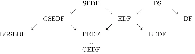
In Figure 1, we indicate the relationship between the various types of difference families we have defined. If we designateX→Y, this indicates that any example of “X” automatically satisfies the properties of “Y”.
3
Weak AMD Codes
Our goal is to prove lower bounds on the adversary’s optimal success probability, ˆ. Note that a
lower bound on ˆ states that there exists an adversary who wins the relevant game with at least
SEDF DS
. & . &
GSEDF EDF DF
. & . &
BGSEDF PEDF BEDF
↓
[image:12.612.138.479.73.168.2]GEDF
Figure 1: Relationships between various types of difference families
3.1 Bounds for Weak AMD Codes
Theorem 3.1. In any weak (m, n,ˆ)-AMD code, it holds that
ˆ
≥ a(m−1)
m(n−1).
Proof. Suppose the adversary chooses the value ∆ ∈ G \ {0} uniformly at random. For any given
g∈A(s) and for a randomly chosen ∆, the probability that the adversary wins is (a−as)/(n−1).
The success probabilityrandof this random strategy rand is
rand =
X
s
Pr[s] X
g∈A(s)
Pr[E(s) =g]×a−as
n−1
= X
s
Pr[s]×a−as
n−1
= a
n−1−
X
s
as
m(n−1) (because the sources are equiprobable) = a
n−1−
a m(n−1)
= a(m−1)
m(n−1).
Corollary 3.2. In anyk-uniform weak (m, n,ˆ)-AMD code, it holds that
ˆ
≥ k(m−1)
n−1 .
Proof. Note thata=km in ak-uniform code and apply Theorem 3.1.
Definition 3.1. We will define a weak AMD code that meets the bound of Theorem 3.1 (or Corollary 3.2, in the case that the code is k-uniform) with equality to be R-optimal. Here, “R” is used to indicate that rand is an optimal strategy.
Corollary 3.3. [5, Theorem 2.2] In any weak (m, n,ˆ)-AMD code, it holds that
ˆ
≥ m−1
Proof. Note thata≥m and apply Theorem 3.1.
Remark: The bound of Corollary 3.3 is met with equality only if the code is deterministic. Here is a new bound for weak AMD codes, that arises from a different adversarial strategy.
Theorem 3.4. In any weak (m, n,ˆ)-AMD code, it holds that
ˆ
≥ 1
a.
Proof. We consider the following strategy guess for the adversary:
1. Find the encoding ˆg∈ Athat occurs with the highest probability. Observe that Pr[ˆg]≥1/a.
2. Pick a ∆ that will work for the particular encoding ˆg.
Clearly, the success probability guess of the strategyguess is equal toPr[ˆg]≥1/a.
Definition 3.2. We will define a weak AMD code that meets the bound of Theorem 3.4 with equality to be G-optimal. Here, “G” is used to indicate thatguess is an optimal strategy.
Theorem 3.5. In any weak (m, n,ˆ)-AMD code, it holds that
ˆ
2 ≥ m−1
m(n−1).
Proof. Multiply the bounds proven in Theorems 3.1 and 3.4.
A code that meets the bound of Theorem 3.5 with equality is simultaneously R-optimal and G-optimal.
3.2 Optimal Weak AMD Codes
In this section, we consider weak AMD codes that are R-optimal and/or G-optimal. Recall that a weak AMD code is R-optimal if ˆ=a(m−1)/(m(n−1)) and it is G-optimal if ˆ= 1/a.
3.2.1 R-Optimal Weak AMD Codes
First, we consider R-optimality. Consider the strategyg7→g+ ∆, where ∆6= 0, and let∆ denote
the success probability of this strategy. Clearly, we have
ˆ
= max{∆: ∆6= 0}. (6)
For any ∆6= 0, define
Good(∆) ={g∈ G0 :g∈A(s) andg+ ∆∈A(s0),where s0 6=s}. (7)
Lemma 3.6. For any ∆6= 0, it holds that
∆= X
g∈Good(∆)
Pr[g]. (8)
Proof. It is clear that
∆ = Pr[g∈Good(∆)]
= X
g∈Good(∆)
Pr[g].
Theorem 3.7. A weak AMD code is R-optimal if and only if ∆ =a(m−1)/(m(n−1)) for all
∆6= 0.
Proof. Suppose we have an R-optimal weak AMD code. It is not hard to compute
X
∆6=0
∆ = X
∆6=0 X
g∈Good(∆)
Pr[g]
= X
g∈G0
Pr[g]× |{∆ :g∈Good(∆)}|
= X
s∈S
X
g∈A(s)
Pr[s]Pr[E(s) =g]× |{∆ :g∈Good(∆)}|
= X
s∈S
Pr[s] X
g∈A(s)
Pr[E(s) =g](a−as)
= X
s∈S
Pr[s](a−as)
= X
s∈S
1
m(a−as)
= a(m−1)
m .
Therefore the average of the quantities ∆ (∆ 6= 0) is equal to a(m−1)/(m(n−1)). In order to
have ˆ=a(m−1)/(m(n−1)), it must be the case that∆=a(m−1)/(m(n−1)) for all ∆6= 0.
We next present a method of constructing R-optimal weak AMD codes.
Theorem 3.8. Suppose there is an (n, m;k1, . . . , km;λ1, . . . , λm)-GSEDF. Then there is an
(R-optimal) weak (m, n, a(m−1)/(m(n−1)))-AMD code, where a=Pm i=1ki.
Proof. Suppose the GSEDF is given byA1, . . . , Am. Leta=Pmi=1ki. Observe that
ki(a−ki) =λi(n−1) (9)
for 1≤i≤m. Let S ={s1, . . . , sm} be a set of m sources. For 1≤i≤m, defineA(si) =Ai and
all ∆6= 0. We have
∆ =
X
g∈Good(∆)
Pr[g]
= m X i=1 1 m × λi ki = 1 m m X i=1
a−ki
n−1 from (9)
= 1
m(n−1)
m X
i=1
(a−ki)
= a(m−1)
m(n−1).
In fact, we can obtain R-optimal weak AMD codes from a weaker type of difference family, namely, a PEDF.
Theorem 3.9. Suppose there is an(n, m;c1, . . . , c`;k1, . . . , k`;λ1, . . . , λ`)-PEDF. Then there is an
(R-optimal) weak(m, n, a(m−1)/(m(n−1)))-AMD code, where a=P`h=1chkh.
Proof. We omit the proof, which is similar to the proof of Theorem 3.8.
It is interesting to note that the we do not necessarily obtain an R-optimal AMD code if we start from an arbitrary generalized external difference family. As an example, suppose we construct an AMD code with equiprobable encoding for two sources using the GEDF presented in Example 2.4. Here it is easy to compute
1=
1 4 >
a(m−1)
m(n−1) = 5×1 2×12 =
5 24, so this code is not R-optimal
It is an open problem to characterize R-optimal (weak) AMD codes. The following example illustrates that the converse of Theorem 3.9 is not true in general. That, is we can construct R-optimal codes that do not come from PEDFs.
Example 3.1. LetS={1,2,3,4}and letG =Z10. The encoding functionE is defined byE(1) = 0,
E(2) = 5, E(3)∈R{1,9} and E(4)∈R{2,3}.
Suppose the adversary chooses ∆ = 5; then the adversary wins if s∈ {1,2}, which occurs with probability 1/2. Suppose the adversary chooses ∆ = 1; then the adversary succeeds if s ∈ {1,3}, which occurs with probability 1/2. Suppose the the adversary chooses ∆ = 2; then the adversary succeeds if s= 1, ifs= 3 and E(s) = 1, or if s= 4 andE(s) = 3. The success probability here is
1 4 + 1 4 × 1 2+ 1 4× 1 2 = 1 2.
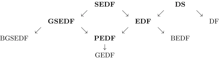
SEDF DS
. & . &
GSEDF EDF DF
. & . &
BGSEDF PEDF BEDF
↓
[image:16.612.132.485.72.168.2]GEDF
Figure 2: Difference families that yield R-optimal weak AMD codes (indicated in boldface type)
We can give a tight characterization of k-regular R-optimal weak AMD codes, however, as follows.
Theorem 3.10. An (R-optimal) k-regular weak (m, n, k(m−1)/(n−1))-AMD code is equivalent to an (n, m, k, λ)-EDF.
Proof. Suppose A1, . . . , Am is an (n, m, k, λ)-EDF. Let S = {s1, . . . , sm} be a set of m sources.
For 1 ≤ i ≤ m, suppose the encoding function E(si) is equiprobable. The resulting weak AMD
code is k-regular. Choose any ∆ ∈ G, ∆ 6= 0. The strategy g7→ g+ ∆ succeeds with probability
∆=λ/(km) =k(m−1)/(n−1). (In fact, this follows from Theorem 3.9.)
Conversely, suppose we have an R-optimal k-regular weak AMD code. Then it must be the case that ∆ =k(m−1)/(n−1) for all ∆6= 0. Using the fact that the code is a k-regular AMD,
we have
k(m−1)
n−1 =∆=Pr[E(s)∈Good(∆)] =
|Good(∆)|
km .
Therefore,
|Good(∆)|= k
2m(m−1)
n−1 .
It then follows that{A(s) :s∈ S}is an (n, m, k, λ)-EDF, where λ=k2m(m−1)/(n−1).
In Figure 2 we indicate the types of difference families that yield R-optimal weak AMD codes. This summarizes the results proven in this section.
3.2.2 G-Optimal Weak AMD Codes
Now we turn to G-optimality. We have the following characterization of G-optimal weak AMD codes.
Theorem 3.11. A (G-optimal) weak m, n,1a-AMD code is equivalent to an (n, m, k,1)-BEDF, where a=km.
Proof. SupposeA1, . . . , Amis an (n, m, k,1)-BEDF. LetS ={s1, . . . , sm}be a set ofmsources. For
1≤i≤m, define an encoding functionE(si) which chooses an element ofAi uniformly at random.
Choose any ∆∈ G, ∆6= 0. The strategy g7→g+ ∆ succeeds with probability∆≤1/(km) = 1/a,
since there is at most one occurrence of the difference ∆ in the BEDF. Further, if ∆ ∈ D(Aj, Ai)
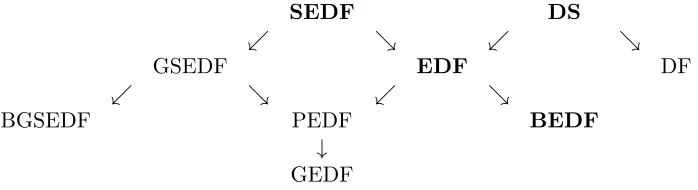
SEDF DS
. & . &
GSEDF EDF DF
. & . &
BGSEDF PEDF BEDF
↓
[image:17.612.133.482.73.168.2]GEDF
Figure 3: Difference families with λ = 1 that yield G-optimal weak AMD codes (indicated in boldface type)
Conversely, suppose we have a G-optimal weak AMD code. From the proof of Theorem 3.4, we see that all encodings must occur with the same probability, 1/a. Since the sources are equiprobable, this happens only if the code is k-regular with k=a/m. Now we claim that {A(s) :s∈ S} is an (n, m, k,1)-BEDF. This is easy to see, because if some difference occurred more than once, it would immediately follow that ≥2/a.
Now we characterize k-regular weak AMD codes that are simultaneously R-optimal and G-optimal.
Theorem 3.12. A k-regular weak AMD code that is simultaneously R-optimal and G-optimal is equivalent to an (n, m, k,1)-EDF.
Proof. From Theorem 3.5, the code has success probability qm(nm−−11). In order for this to occur, the bounds of Corollary 3.2 and 3.4 both must hold with equality. Therefore the AMD code is simultaneously an (n, m, k, λ)-EDF (from Theorem 3.10) and an (n, m, k,1)-BEDF (from Theorem 3.11). Hence, it is an (n, m, k,1)-EDF.
In Figure 3 we indicate the types of difference families that yield G-optimal weak AMD codes. Note that the relevant difference families are assumed to have λ= 1 in this figure.
4
Strong AMD Codes
We begin by focussing on the success probability of the adversary when the source is fixed to bes. Let ˆs be the success probability of the optimal strategy for the given sources.
Theorem 4.1. In any strong AMD code, it holds that
ˆ
s ≥
a−as
n−1
for any sources∈ S.
Proof. As in the proof of Theorem 3.1, we consider a random strategy, i.e., ∆ 6= 0 is chosen uniformly at random. Given that the source is s, it is easy to see that the success probability of this strategy will be
a−as
Definition 4.1. We will define a strong AMD code that meets the bound of Theorem 4.1 with equality for every possible source s to be R-optimal. Again, “R” is used to indicate that choosing
∆6= 0 uniformly at random is an optimal strategy.
Corollary 4.2. In any strong (m, n,ˆ)-AMD code, it holds that
ˆ
≥ a−as0
n−1 ,
where as0 = min{as :s∈ S}.
Proof. The quantity (a−as)/(n−1) is maximized when as is minimized.
If the code is k-uniform, then the previous bound takes a simpler form.
Corollary 4.3. In anyk-uniform strong (m, n,ˆ)-AMD code, it holds that
ˆ
≥ k(m−1)
n−1 .
Proof. Here as=k for allsand a=km. Apply Corollary 4.2.
Theorem 4.4. In any strong AMD code, it holds thatˆs≥1/as,for any source s∈ S.
Proof. Given any source s, the adversary can try to guess the encoded message E(s) that is out-put. The adversary will maximize his probability of success by choosing g such that Pr[g |s] is maximized. Note that there exists a g such that Pr[g|s]≥1/as. Then the adversary can choose
∆ such thatg+ ∆∈ G0\A(s). The success probability of this strategy is clearly at least 1/as.
Definition 4.2. We will define a strong AMD code that meets the bound of Theorem 4.4 with equality for every possible source s to be G-optimal. Again, “G” is used to indicate that guessing the most likely encoding is an optimal strategy.
Corollary 4.5. In any strong (m, n,ˆ)-AMD code, it holds that ˆ≥ 1/as0, where as0 = min{as :
s∈ S}.
Proof. The quantity 1/as is maximized when as is minimized.
In the case of a k-regular code, we have the following corollary.
Corollary 4.6. In anyk-regular strong (m, n,ˆ)-AMD code, it holds thatˆ≥1/k.
We now have an easy proof of the following previously known bound.
Theorem 4.7. [5, Theorem 2.2] In anyk-uniform, strong (m, n,ˆ)-AMD code, it holds that
ˆ
2≥ m−1
n−1.
Proof. From Corollary 4.3, we have
ˆ
≥ k(m−1)
n−1 .
Furthermore, from Corollary 4.6, we have ˆ≥1/k.Multiplying these two inequalities, we get
ˆ
2≥ m−1
Remark: We will determine in Theorem 4.14 necessary and sufficient conditions for the bound of Theorem 4.7 to be met with equality in all nontrivial cases, i.e., when ˆ <1.
4.1 Optimal Strong AMD Codes
4.1.1 R-Optimal Strong AMD Codes
Suppose the sourcesis fixed. Consider the strategy g7→g+ ∆, where ∆ 6= 0. Let∆,s denote the
success probability of this strategy. Then it is clear that
ˆ
s= max{∆,s : ∆6= 0}. (10)
For any ∆6= 0, define
Good(∆, s) ={g:g∈A(s) andg+ ∆∈A(s0),wheres06=s}. (11)
This is the same definition as (7), except that sis now fixed.
Lemma 4.8. For any ∆6= 0, it holds that
∆,s=
X
g∈Good(∆,s)
Pr[E(s) =g]. (12)
Proof. It is clear that
∆,s = Pr[E(s)∈Good(∆, s)]
= X
g∈Good(∆,s)
Pr[E(s) =g].
Theorem 4.9. In any strong AMD code,ˆs= (a−as)/(n−1)if and only if∆,s = (a−as)/(n−1)
for all ∆6= 0.
Proof. Suppose we have an AMD code where ˆs= (a−as)/(n−1). It is not hard to compute
X
∆6=0
∆,s = X
∆6=0
X
g∈Good(∆,s)
Pr[E(s) =g]
= X
g∈A(s)
Pr[E(s) =g]× |{∆ :g∈Good(∆, s)}|
= X
g∈A(s)
Pr[E(s) =g]×(a−as)
= a−as.
Therefore the average of the quantities ∆,s (∆6= 0) is equal to (a−as)/(n−1). In order to have
ˆ
s= (a−as)/(n−1), it must be the case that∆,s = (a−as)/(n−1) for all ∆6= 0.
Theorem 4.10. Suppose there is an (n, m;k1, . . . , km;λ1, . . . , λm)-GSEDF. Then there is an
Proof. Suppose the GSEDF is given byA1, . . . , Am. LetS ={s1, . . . , sm}be a set ofmsources. For
1≤i≤m, defineA(si) =Ai, soasi =ki, and suppose the encoding functionE(si) is equiprobable.
We show that∆,si = (a−asi)/(n−1) for 1≤i≤m and all ∆6= 0. We have
∆,si =
X
g∈Good(∆,si)
Pr[g]
= λi
ki
= a−ki
n−1 from (9) = a−asi
n−1 .
It is possible to prove a converse to Theorem 4.10 in the case where the AMD code has equiprob-able encoding.
Theorem 4.11. Suppose there is an R-optimal strong AMD code with equiprobable encoding. Then the setsA(s) (s∈ S) form an (n, m;k1, . . . , km;λ1, . . . , λm)-GSEDF.
Proof. Suppose the sources are denoted S ={s1, . . . , sm}. Fix a value i, 1≤i≤m and let ∆6= 0.
We have
∆,si =
a−asi
n−1
= X
g∈Good(∆,si)
Pr[g]
= |Good(∆, si)|
asi
.
Therefore, for a fixed valuei, we have
|Good(∆, si)|=
asi(a−asi)
n−1 for all ∆6= 0. This says that
D(A(si),G0\A(si)) =λi(G \ {0}),
where
λi=
asi(a−asi)
n−1 .
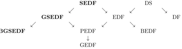
SEDF DS
. & . &
GSEDF EDF DF
. & . &
BGSEDF PEDF BEDF
↓
[image:21.612.135.481.72.168.2]GEDF
Figure 4: Difference families that yield R-optimal strong AMD codes (indicated in boldface type)
4.1.2 G-Optimal Strong AMD Codes
Now we turn to G-optimality. We have the following characterization of G-optimal strong AMD codes.
Theorem 4.12. A G-optimal strong AMD code is equivalent to an (n, m;k1, . . . , km; 1, . . . ,1)
-BGSEDF.
Proof. Suppose A1, . . . , Am is an (n, m;k1, . . . , km; 1, . . . ,1)-BGSEDF. Let S ={s1, . . . , sm} be a
set of m sources. For 1 ≤i≤ m, define an encoding function E(si) which chooses an element of
Ai uniformly at random. Let 1≤i≤m and choose any ∆∈ G \ {0}. Given that the source is si,
the strategy g7→g+ ∆ succeeds with probability at most 1/asi, since there is at most oneg∈Ai
such that g+ ∆∈ Aj and j 6= i. Further, there exists a ∆ 6= 0 such that this strategy succeeds
with probability 1/asi.
Conversely, suppose we have a G-optimal strong AMD code. Let s ∈ S. From the proof of Theorem 4.4, it is easy to see that all encodings ofsoccur with the same probability 1/|A(s)|. Now we claim that{A(s) :s∈ S}is an (n, m;k1, . . . , km; 1, . . . ,1)-BGSEDF. Suppose that there existed
two different valuesg, g0 ∈Ai such thatg+ ∆∈Aj,g0+ ∆∈Aj0 andj, j0 6=i. It would then follow
that ˆs≥2/|A(s)|, which is a contradiction.
Now we show thatk-regular strong AMD codes withm≥3 cannot be simultaneously R-optimal and G-optimal.
Theorem 4.13. There does not exist a strong AMD code withm≥3 and ˆ <1 that is simultane-ously R-optimal and G-optimal.
Proof. Since the code is G-optimal, it follows from Theorem 4.12 and its proof that the code has equiprobable encoding and is derived from (n, m;k1, . . . , km; 1, . . . ,1)-BGSEDF. Now, since the code
is R-optimal and it has equiprobable encoding, Theorem 4.11 shows that the code is derived from (n, m;k1, . . . , km;λ1, . . . , λm)-GSEDF. Thus we have an (n, m;k1, . . . , km; 1, . . . ,1)-BGSEDF that
is also an (n, m;k1, . . . , km;λ1, . . . , λm)-GSEDF, so it must in fact be an (n, m;k1, . . . , km; 1, . . . ,
1)-GSEDF. This implies thatki(a−ki) =n−1 for alli. Givenaand n, the equation x(a−x) =n−1
has at most two distinct roots, and these roots sum toa. Suppose thatki6=kj for somei, j. Then
ki+kj = a, which implies that m = 2, a contradiction. Hence the code is k-uniform and the
SEDF DS
. & . &
GSEDF EDF DF
. & . &
BGSEDF PEDF BEDF
↓
[image:22.612.134.484.73.168.2]GEDF
Figure 5: Difference families with λ = 1 that yield G-optimal strong AMD codes (indicated in boldface type)
Theorem 4.14. There exists a k-uniform, strong (m, n,ˆ)-AMD code with ˆ2 = mn−−11 < 1 if and only ifm= 2 andn=k2+ 1.
Proof. Here we are considering k-uniform strong AMD codes that are simultaneously R-optimal and G-optimal. From the proof of Theorem 4.13, we see thatm = 2 and k(a−k) = n−1. Since
a= 2k, we have n= k2+ 1. Conversely, if m = 2 and n =k2 + 1, then Example 2.2 shows the existence of a (k2+ 1,2;k; 1)-SEDF. This yields a strong AMD code with ˆ= 1/k, as desired.
Figure 5 shows the types of difference families that yield G-optimal strong AMD codes. The relevant difference families are assumed to haveλ= 1 in this figure.
5
Conclusion
We have studied weak and strong AMD codes that provide optimal protection against two specific adversarial substitution strategies. These codes are termed “R-optimal” and “G-optimal”. We have considered various types of generalized difference families and determined when they yield optimal and/or G-optimal AMD codes. As well, we have proven in certain situations that R-optimal and/or G-R-optimal AMD codes imply the existence of the relevant difference families, thus providing a combinatorial characterization of the AMD codes under consideration.
It is an interesting open problem to construct additional examples of these generalized difference families. In particular, we ask if there are any examples of strong external difference families with
k >1 andm >2. We are unaware of any such examples at the present time.
We should mention that there have been other bounds proven for AMD codes, in particular, for special classes of AMD codes, includingsystematicAMD codes. For example, [6, Proposition 6] uses a coding-theoretic approach to prove a necessary condition for the existence of a systematic AMD code. We focussed on bounds which can be met with equality if appropriate difference sets and difference families exist. We do not know if there are any natural connections between difference families and “optimal” systematic AMD codes.
References
[2] Y. Chang and C. Ding. Constructions of external difference families and disjoint difference families.Designs, Codes and Cryptography40 (2006) 67–185.
[3] R. Cramer, Y. Dodis, S. Fehr, C. Padr´o and D. Wichs. Detection of algebraic manipulation with applications to robust secret sharing and fuzzy extractors.Lecture Notes in Computer Science4965(2008), 471–488 (Eurocrypt 2008).
[4] R. Cramer, Y. Dodis, S. Fehr, C. Padr´o and D. Wichs. Detection of algebraic manipulation with applications to robust secret sharing and fuzzy extractors. Cryptology ePrint Archive: Report 2008/030.
[5] R. Cramer, S. Fehr and C. Padr´o. Algebraic manipulation detection codes. Science China Mathematics56(2013), 1349–1358.
[6] R. Cramer. C. Padr´o and C. Xing. Optimal algebraic manipulation detection codes in the constant-error model.Lecture Notes in Computer Science9014(2015), 481–501 (TCC 2015).
[7] F. CuiLing, L. JianGuo and S. XiuLing. Constructions of optimal difference systems of sets.
Science China Mathematics54(2011), 173–184.
[8] Y. Fujiwara K. Momihara and M. Yamada. Perfect difference systems of sets and Jacobi sums.Discrete Mathematics 309(2009), 3954–3961.
[9] Y. Fujiwara and V.D. Tonchev. High-rate self-synchronizing codes. IEEE Transactions on Information Theory 59(2013), 2328–2335.
[10] B. Huang and D. Wu. Cyclotomic constructions of external difference families and disjoint difference families.Journal of Combinatorial Designs 17(2009), 333–341.
[11] J. Lei and C. Fan. Optimal difference systems of sets and partition-type cyclic difference packings.Designs, Codes and Cryptography58(2011), 135–153.
[12] V.I. Levenshtein. One method of constructing quasilinear codes providing synchronization in the presence of errors.Problems of Information Transmission 7 (1971), 215–222.
[13] W. Ogata and K. Kurosawa. Optimum secret sharing scheme against cheating.Lecture Notes in Computer Science1070(1996), 200–211 (EUROCRYPT ’96).
[14] W. Ogata, K. Kurosawa, D.R. Stinson and H. Saido. New combinatorial designs and their applications to authentication codes and secret sharing schemes. Discrete Mathematics 279
(2004), 383–405.
[15] W. Ogata, K. Kurosawa and D.R. Stinson. Optimum secret sharing scheme secure against cheating.SIAM Journal on Discrete Mathematics20 (2006), 79–95.
[16] G.J. Simmons. Authentication theory/coding theory.Lecture Notes in Computer Science196
(1985), 411–431 (Proceedings of Crypto ’84).