A distance test of normality for a wide class of stationary processes

BIROn - Birkbeck Institutional Research Online

Psaradakis, Zacharias and Vavra, Marian (2015) A distance test of normality

for a wide class of stationary processes. Working Paper. Birkbeck College,

University of London, London, UK.

Downloaded from:

Usage Guidelines:

Please refer to usage guidelines at or alternatively

ISSN 1745-8587

Department of Economics, Mathematics and Statistics

BWPEF 1513

A Distance Test of Normality for

a Wide Class of Stationary

Processes

Zacharias Psaradakis

Birkbeck, University of London

Marián Vávra

National Bank of Slovakia

September 2015

B

ir

kb

ec

k

W

or

ki

ng

P

a

per

s

in

E

co

n

om

ics

&

Fi

n

a

nc

A Distance Test of Normality for a

Wide Class of Stationary Processes

Zacharias Psaradakis

Department of Economics, Mathematics and Statistics

Birkbeck, University of London

E-mail:

[email protected]

Mari´

an V´

avra

Advisor to the Governor and Research Department

National Bank of Slovakia

E-mail:

[email protected]

September 2015

Abstract

Key Words: Distance test; Fractionally integrated process; Sieve bootstrap; Nor-mality.

1

Introduction

Testing whether a sample of observations comes from a Gaussian distribution is a prob-lem that has attracted a great deal of attention over the years. This is not perhaps surprising in view of the fact that normality is a common maintained assumption in a wide variety of statistical procedures, including estimation, inference and forecast-ing procedures. In model buildforecast-ing, a test for normality is often a useful diagnostic for assessing whether a particular type of stochastic model may provide an appropri-ate characterization of the data (for instance, non-linear models are unlikely to be an adequate approximation to a time series having a Gaussian one-dimensional marginal distribution). Normality tests may also be useful in evaluating the validity of different hypotheses and models to the extent that the latter rely on or imply Gaussianity, as is the case, for example, with some option pricing, asset pricing, and dynamic stochastic general equilibrium models found in the economics and finance literature.1

Although most of the voluminous literature on the subject of testing for univari-ate normality has focused on the case of independent, identically distributed (i.i.d.) observations (see Thode (2002) for an extensive review), a small number of tests which are valid for dependent data have also been considered. These include tests based on the bispectrum (e.g., Hinich (1982); Nusrat and Harvill (2008); Berg, Paparoditis, and Politis (2010)), the characteristic function (Epps (1987)), moment conditions implied by Stein’s characterization of the Gaussian distribution (Bontemps and Meddahi (2005)), and classical measures of skewness and kurtosis involving standardized third and fourth central moments (Lobato and Velasco (2004); Bai and Ng (2005)). A feature shared by these tests is that they all rely on asymptotic results obtained under dependence condi-tions which typically require the autocovariances of the data to decay towards zero, as the lag parameter goes to infinity, sufficiently fast to be (at least) absolutely summable. It has long been recognized, however, that such short-range dependence conditions may

1_{Kilian and Demiroglu (2000) and Bontemps and Meddahi (2005) give examples from economics,}

not accord well with the slowly decaying autocovariances of many observed time series. The purpose of this paper is to discuss a test for normality which may be used in the presence of not only short-range dependence but also long-range dependence and an-tipersistence. The defining characteristic of stochastic processes with such dependence structures is that their autocovariances decay to zero as a power of the lag parameter and, in the case of long-range dependence, slowly enough to be non-summable. Models that allow for long-range dependence have been found to be useful for modelling data occurring in fields as diverse as economics, geophysics, hydrology, meteorology, and telecommunications.2

The normality test we consider here is based on the Anderson–Darling distance statistic involving the weighted quadratic distance of the empirical distribution func-tion of the data from a Gaussian distribufunc-tion funcfunc-tion (Anderson and Darling (1952)). Unlike tests based on measures of skewness and kurtosis, which can only detect devia-tions from normality that are reflected in the values of such measures, normality tests based on the empirical distribution function are known to be consistent against any fixed non-Gaussian alternative. The Anderson–Darling test also fares well in small-sample power comparisons for i.i.d. data relatively to the popular correlation test of Shapiro and Wilk (1965) and the moment-based tests of Bowman and Shenton (1975) and Jarque and Bera (1987) (see, e.g., Stephens (1974) and Thode (2002, Ch. 7)). Furthermore, the Anderson–Darling test is superior, in terms of asymptotic relative efficiency, to distance tests such as those based on the (unweighted) Cram´er–von Mises and Kolmogorov–Smirnov statistics (Koziol (1986); Arcones (2006)).

Our analysis extends earlier work by considering the case of correlated data from (strictly stationary) fractionally integrated processes, which may be short-range depen-dent, long-range dependent or antipersistent depending on the value of their dependence parameter. Unfortunately, however, inference based on conventional large-sample ap-proximations is anything but straightforward in such a setting because the weak limit

2_{A summary of some of the empirical evidence on long-range dependence can be found in the}

of the null distribution of the test statistic, as well as the appropriate norming factor, depend on the unknown dependence parameter of the data and on the particular esti-mators of location and scale parameters that are used in the construction of the test statistic.

As a practical way of overcoming these difficulties, we propose to use the bootstrap to estimate the null sampling distribution of the Anderson–Darling distance statistic and thus obtain estimates of P-values and/or critical values for a normality test. Our approach relies on the autoregressive sieve bootstrap, which is based on the idea of approximating the data-generating mechanism by an autoregressive sieve, that is a sequence of autoregressive models that increase in order as the sample size increases without bound (Kreiss (1992); B¨uhlmann (1997)). The bootstrap-based normality test is easy to implement and requires knowledge (or estimation) of neither the value of the dependence parameter of the data nor of the appropriate norming factor for the test statistic. Furthermore, the bootstrap scheme is the same under short-range dependence, long-range dependence and antipersistence.

We note that Beran and Ghosh (1991) and Boutahar (2010) obtained some results relating to the asymptotic behaviour of moment-based and distance-based statistics under long-range dependence, but they did not discuss how operational tests for nor-mality might be constructed. To the best of our knowledge, the problem of developing an operational normality test which is valid for data that are neither independent nor short-range dependent has not been tackled in the existing literature.

2

Assumptions and Test Statistic

SupposeXn :={X1, X2, . . . , Xn}are consecutive observations from a strictly stationary

stochastic process X:={Xt}t∈Z satisfying

Xt−µ=

∞

X

j=0

ψjεt−j, t∈Z, (1)

for some µ ∈ _R, where {ψj}j>0 is a square-summable sequence of real numbers (with

ψ0 = 1) and{εt}t∈_Zis a sequence of i.i.d., real-valued, zero-mean random variables with

varianceσ2 ∈(0,∞). The objective is to test the hypothesis that the one-dimensional marginal distribution ofX is Gaussian, that is

F(µ+γ₀1/2x)−Φ(x) = 0 for all x∈_R, (2)

where γk := Cov(Xk, X0) = σ2

P∞

j=0ψj+|k|ψj for k ∈ Z, F is the distribution function

ofX0, and Φ denotes the standard-normal distribution function. Note that Gaussianity

of the distribution ofε0 is sufficient for (2) to hold.

To allow for different types of dependence, it will be maintained throughout that the transfer function ψ(z) := P∞

j=0ψjz j_{, z ∈}

C, associated with (1) satisfies

ψ(z) = (1−z)−dπ(z), |z|<1, (3)

for some real |d|< 1₂, where π(z) :=P∞

j=0πjzj and {πj}j>0 is an absolutely summable

sequence of real numbers such that π(0) = 1 and π(1) 6= 0. Under (1) and (3), X

is a fractionally integrated process with dependence (memory/fractional differencing) parameterd. Using the Maclaurin series expansion

(1−z)−d =

∞

X

j=0

Γ(j +d) Γ(d)Γ(j+ 1)z

j_{, |z|<1, d6= 0,}

where Γ denotes the gamma function, it is not difficult to see that, ford6= 0,

ψj = j

X

h=0

πj−hΓ(h+d)

and so ψj ∼ {π(1)/Γ(d)}jd−1 as j → ∞ (the tilde signifies that the limiting value of

the ratio of two terms is 1). Hence, sinceγk ∼C|k|2d−1 as|k| → ∞ford6= 0 and some

C 6= 0, the series P∞

k=−∞γk diverges for 0 < d < 1₂ and X is long-range dependent;

if −1

2 < d < 0, then

P∞

k=−∞γk = 0 and X is antipersistent. Short-range dependence

corresponds to d = 0, with P∞

k=−∞γk = {σπ(1)}2. The class of stochastic processes

defined by (1) and (3) is rich enough to include a wide range of processes with slowly decaying autocovariances. A prominent example are causal autoregressive fractionally integrated moving average (ARFIMA) processes withπ(z) =ϑ(z)/ϕ(z),ϑ(z) andϕ(z) being relatively prime polynomials of finite order with ϕ(z) 6= 0 for |z| ₆ 1 (see, e.g., Palma (2007, Sect. 3.2)).

The test for the hypothesis in (2) considered here is based on the Anderson– Darling distance statistic

A:=

Z ∞

−∞

{Fˆ( ¯X+ ˆγ₀1/2x)−Φ(x)}2

Φ(x){1−Φ(x)} dΦ(x), (4)

where ˆF(x) := n−1Pn

t=1I(Xt6x),x∈R, is the empirical distribution function ofXn,

¯

X :=n−1Pn

t=1Xt, ˆγk :=n

−1Pn−|k|

t=1 (Xt+|k|−X¯)(Xt−X¯) for|k|6n−1, and Idenotes

the indicator function. Note thatA may equivalently be expressed as

A =−1−n−2 n

X

t=1

(2t−1) [log Φ(Yt) + log{1−Φ(Yn−t+1)}], (5)

whereYt := ˆγ

−1/2

0 (Xn:t− X¯) and Xn:t is the t-th order statistic from Xn.

As is well known, the asymptotic null distribution of distance statistics such asAis closely related to the weak limit, asntends to infinity, of (a suitably normalized version of) the random function ˆK(x) := ˆF(x)−Φ(ˆγ₀−1/2(x−X¯)), x ∈ _R (see, e.g., Shorack and Wellner (1986, Ch. 5) for the case of i.i.d. data). However, unless one is dealing with the classical problem of testing a simple null hypothesis (µandγ0 known) for i.i.d.

the estimators ofµand γ0 used in the construction of ˆK (see Beran and Ghosh (1991);

Ho (2002); Kulik (2009)). For example, when ε0 is normally distributed, the random

functionK(x) := ˆF(x)−Φ(γ₀−1/2(x−µ)),x∈_R, converges weakly to a non-degenerate Gaussian process at the usual √n rate for d = 0 (Doukhan and Surgailis (1998)) and to a semi-deterministic Gaussian process at the slower rate n(1−2d)/2 _{for 0 < d <} 1

2

(cf. Dehling and Taqqu (1989); Giraitis and Surgailis (1999)). Replacing µ and γ0

by estimates improves the rate of convergence under long-range dependence, with ˆK

converging at rate√nfor 0₆d < 1₃ (cf. Beran and Ghosh (1991)). The dependence of the appropriate norming factors and asymptotic distributions on the unknown value of the dependence parameter, combined with the complicated covariance structure of the relevant limiting processes, clearly make inference based on conventional large-sample asymptotics for A extremely cumbersome.3

As a practical way of circumventing the problems mentioned above, we propose to use an autoregressive sieve bootstrap procedure to obtain P-values and/or critical values for the normality test based onA. The principal advantage of the sieve bootstrap is that it can used to approximate the sampling properties ofA without knowledge or estimation of the dependence parameter and is valid for all|d|< 1₂. Moreover, because bootstrap approximations are constructed from replicates of A, there is no need to derive analytically, nor to make assumptions about, the appropriate norming factor for

A or its asymptotic null distribution.

3

Autoregressive Sieve Bootstrap Approximation

The autoregressive sieve bootstrap is motivated by the observation that, under (1), (3) and the additional assumption that π(z)6= 0 for |z|₆1,X admits the representation

∞

X

j=0

φj(Xt−j −µ) = εt, t ∈Z, (6)

3_{It is worth remarking that similar difficulties also arise in the case of moment-based skewness and}

for a square-summable sequence of real numbers {φj}j>0 (with φ0 = 1) such that

φ(z) := P∞

j=0φjz

j _{= (1−z)}d_{/π(z) for |z| < 1 (with φ}

j ∼ {π(1)Γ(−d)}−1j−d−1 as

j → ∞ when d 6= 0). The idea is to approximate (6) by a finite-order autoregressive model and use this as the basis of a semi-parametric bootstrap scheme. If the order of the autoregressive approximation is allowed to increase simultaneously withnat an ap-propriate rate, the distribution of the process in (6) will be matched asymptotically (cf. Kreiss (1992); B¨uhlmann (1997); Kapetanios and Psaradakis (2006); Poskitt (2008)).

It is important to point out that, as discussed in Poskitt (2007), the autoregressive representation (6) provides a meaningful approximation even if π(z) has zeros in the disk|z|<1. In this case, the transfer function φ(z) associated with (6) may be viewed as arising, not from the inversion of ψ(z), but as the limit of Pp

j=0φpjzj (φp0 := 1)

as p → ∞, where, for any integer p _> 1, (−φp1, . . . ,−φpp) are the coefficients of the

best (in the mean-square sense) linear predictor ofXt based on (Xt−1, . . . , Xt−p). Since γ0 >0 andγk→0 as|k| → ∞under (1) and (3), (φp1, . . . , φpp) are uniquely determined

as the solution of the set of equations Pp

j=0φpjγk−j = 0 (k = 1, . . . , p) (Brockwell and

Davis (1991, Corollary 5.1.1)), and are such that Pp

j=0φpjz

j _{6= 0 for |z|}

6 1 and Var[Pp

j=0φpj(Xt−j−µ)]→σ2 asp→ ∞.

The bootstrap procedure used to approximate the sampling properties of the statisticA under the normality hypothesis is as follows. For a positive integer p (cho-sen as a function of n so that p−1 +n−1p → 0 as n → ∞), let ( ˆφp1, . . . ,φˆpp) and

ˆ

σp be estimators (based on Xn) of the coefficients and the noise standard deviation,

respectively, of an autoregressive model of order p for Xt−X¯. Bootstrap replicates X∗ :={X∗

t}t∈_Z of X are then defined via the recursion

p

X

j=0

ˆ

φpj(Xt∗−j −X¯) = ˆσpε∗t, t∈Z, (7)

where ˆφp0 := 1 and {ε∗t}t∈Z are i.i.d. standard-normal random variables

(indepen-dent of Xn). Finally, the bootstrap analogue A∗ of A is defined as in (4) but with X∗_n := {X∗

1, X

∗

2, . . . , X

∗

n} replacing Xn. The conditional distribution of A∗, given Xn,

It is worth noting that, by requiring ε∗_t in (7) to be Gaussian, X∗ is constructed in a way which reflects the normality hypothesis under test even though X may not satisfy (2). This is important for ensuring that the bootstrap test has reasonable power against departures from normality (cf. Hall and Wilson (1991); Lehmann and Romano (2005, Sect. 15.6)). The estimator ( ˆφp1, . . . ,φˆpp,σˆp) used in (7) to defineX∗ may be the

Yule–Walker estimator satisfying the equationsPp

j=0φˆpjˆγk−j =δ0,kσˆ 2

p (k = 0,1, . . . , p),

whereδ0,k is Kronecker’s delta, or any other asymptotically equivalent estimator (e.g.,

the least-squares estimator).

Recalling that A may be expressed as in (5), strong consistency of the sieve bootstrap estimator of the null sampling distribution of A follows from Lemma 1, Theorem 2 and Remark 2 of Poskitt (2008) under a suitable assumption about the rate of increase ofp. More specifically, let ρ(H, H∗) := {R1

0 |H

−1_(u)−H∗−1_(u)|2_du}1/2_stand

for the Mallows–Wasserstein distance between the distribution functionH ofAand the conditional distribution functionH∗ofA∗ _givenX

n(withG−1(u) := inf{x:G(x)>u},

0 < u < 1, for a distribution function G). Then, if X satisfies (1) and (3), the distribution of ε0 is Gaussian, and p→ ∞ and (logn)−νp= O(1) as n → ∞ for some

ν_>1, we have ρ(H, H∗)→0 with probability 1 asn → ∞.4

The bootstrap estimator of theP-value for a test that rejects for large values ofA

isP_A∗ := 1−H∗_{(A), and so normality is rejected at a given level of significanceα∈(0,1)}

if P_A∗ ₆ α. Since convergence with respect to ρ implies weak convergence (Bickel and Freedman (1981, Lemma 8.3)), the bootstrap P-value P_A∗ is asymptotically equivalent to theP-value based on the null sampling distribution ofAunder the conditions stated above. While H∗ is unknown, an approximation (of any desired accuracy) can be obtained by Monte Carlo simulation. Specifically, if (A∗

1, . . . ,A∗m) are copies of A∗,

obtained frommindependent bootstrap pseudo-samplesX∗_nfrom (7), then the empirical

4_{Poskitt (2008) considers a bootstrap scheme in which ε}∗

t in (7) is drawn from the empirical

dis-tribution of the residuals ˆεt:=P p

j=0φˆpj(Xt−j−X¯) (t=p+ 1, . . . , n), standardized to have mean 0

distribution function of (A∗

1, . . . ,A

∗

m) provides an approximation toH

∗_{. Hence, P}∗ Amay

be approximated by ˆP_A∗ :=m−1Pm

i=1I(A

∗

i > A), so that ˆPA∗ → PA∗ with probability 1

asm → ∞. A bootstrap critical value of nominal levelαforAis given by H∗−1_(1−α),

which may be approximated by inf{x:m−1Pm

i=1I(A

∗

i 6x)>1−α}.

In the implementation of the bootstrap procedure in practice, replicates X∗_n may be obtained according to (7) by setting X−∗p+1 = · · · = X0∗ = ¯X, generating n +b

replicates X_t∗, t _> 1, for some large integer b > 0, and then discarding the initial

b replicates to eliminate start-up effects (this procedure, with b = 100, is used in the sequel). The orderpof the autoregressive sieve may be selected by means of the familiar Akaike information criterion (AIC), so that log ˆσ2_p+ 2n−1pis minimized over a suitable range of values of p. Under mild regularity conditions, a data-dependent choice of p

based on the AIC is asymptotically efficient, in the sense defined by Shibata (1980), for all |d| < 1₂ (Poskitt (2007, Theorem 9)); furthermore, it satisfies, with probability 1, the growth conditions required for the asymptotic validity of the sieve bootstrap as long as the maximum allowable sieve order pmax (say) grows to infinity with n so that

(logn)−spmax is eventually bounded for somes>1 (Psaradakis (2015, Proposition 2)).

4

Simulation Study

In this section, we present and discuss the results of a simulation study examining the small-sample properties of the distance-based test of normality under various data-generating mechanisms.

4.1

Experimental Design and Simulation

In the first set of experiments, we examine the performance of the test based on A

under different types of dependence by considering artificial data generated according to the ARFIMA process

M1: (1−0.7L)Xt = (1−0.3L)(1−L)−dεt, d∈ {−0.4,−0.25,0,0.25,0.4},

where {εt} are i.i.d., zero-mean random variables with variance 1 and L denotes the

lag operator.5 _{The distribution of ε}

tis Gaussian (labeled N in what follows), lognormal

(labeled LN), or a member of the family of generalized lambda distributions having inverse distribution functionF−1

ε (u) = λ1+λ2−1{uλ3−(1−u)λ4}; the parameter values

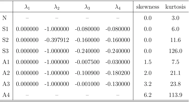
used in the experiments are taken from Bai and Ng (2005) and can be found in Table 1. The distributions S1–S3 are symmetric, whereas A1–A3 and LN are asymmetric.

In the second set of experiments, we assess the robustness of the test based on A

with respect to departures from the linearity assumption underlying the autoregressive sieve bootstrap by using artificial data from the models

M2: Xt= 0.5Xt−1−0.3Xt−1εt−1 +εt,

M3: Xt= (0.9Xt−1+εt)I(|Xt−1|61) + (−0.3Xt−1+ 2εt)I(|Xt−1|>1),

M4: Xt= 0.5Xt−1+εtεt−1.

5_{The stationary solution of M1 satisfies (1) withµ= 0,ψ}

1= 0.4+ζ1andψj = 0.7ψj−1−0.3ζj−1+ζj

M2 is a bilinear model, M3 is a threshold autoregressive model, and M4 is an au-toregressive model with one-dependent, uncorrelated noise. In all three cases, {Xt} is

short-range dependent and does not admit the representation (1) or (6). Furthermore, the distribution ofXt is non-Gaussian even if εt is normally distributed.

In the final set of experiments, we compare the distance test based on A to the moment-based test discussed in Bai and Ng (2005). The latter is based on the statistic

B:=n{τˆ₃−2κˆ2₃+ ˆτ₄−2(ˆκ4−3)2},

where ˆκr := n−1Pn_t=1{ˆγ

−1/2

0 (Xt−X¯)}r (r > 3), and ˆτ32 and ˆτ42 are estimators of the

asymptotic variance of √nκˆ3 and

√

n(ˆκ4 −3), respectively, that are consistent under

normality.6 When {Xt} is a Gaussian process with P

∞

k=−∞|γk| < ∞, the asymptotic

distribution ofB is chi-square with 2 degrees of freedom. Following Bai and Ng (2005), the data-generating mechanism is the autoregressive model

M5: Xt=ϕXt−1+εt, ϕ∈ {0,0.5,0.8}.

For each design point, 1000 independent realizations of {Xt} of length 100 +n,

with n ∈ {100,200,500}, are generated. The first 100 data points of each realization are then discarded in order to eliminate start-up effects and the remainingndata points are used to compute the value of the test statistic of interest. P-values for the distance test are computed from m = 1000 bootstrap replicates of A. The sieve order is taken to be the minimizer of the AIC over the range 1 ₆ p ₆ b(logn)2_{c, where b·c denotes}

the greatest-integer function; the approximating autoregressive model is fitted by least-squares (which is preferred over the Yule–Walker method because it produces estimates that exhibit smaller finite-sample bias).

4.2

Simulation Results

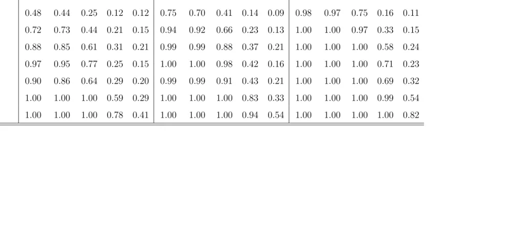
The Monte Carlo rejection frequencies, under M1, of the distance test at 5% significance level (α = 0.05) are reported in Table 2. The null rejection probabilities of the test

6_{Note that the normality test considered by Lobato and Velasco (2004) is also based onB, but their}

choice for ˆτ2

are generally insignificantly different from the nominal level across all values of the dependence parameter. The test also performs well under non-Gaussianity, its rejection frequencies improving with larger sample sizes and smaller values of the dependence parameter. Asymmetry in the distribution ofεtleads, perhaps unsurprisingly, to higher

rejection rates. For long-range dependent data, the test generally suffers a loss in power compared to the short-range dependent or antipersistent cases, a loss which becomes more pronounced the larger the value ofdis. Psaradakis (2015) reports a similar finding for bootstrap-based tests of distributional symmetry about an unspecified centre.

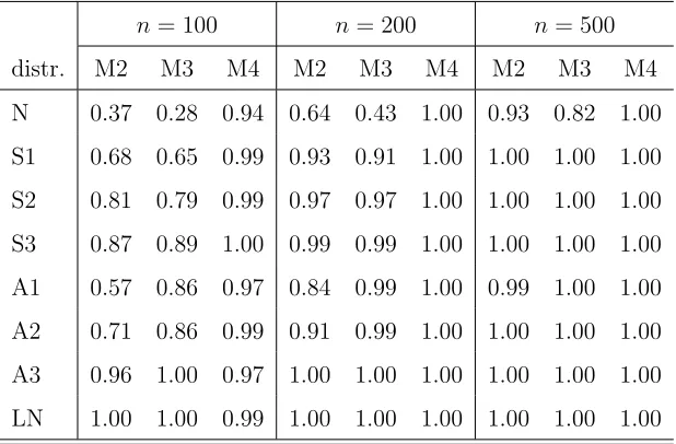
The distance test based on A also works very well for data-generating processes which are not representable as (1) or (6). This can be seen in Table 3, which shows the rejection frequencies of a 5%-level test under M2, M3 and M4. The rejection rate of the distance test exceeds 57% for any design point with non-Gaussian noise, even for the smallest sample size considered.

Let us finally turn to Table 4, which contains the rejection frequencies, at the 5% significance level, of the tests based onA and B under M5; the rejection frequencies of theB test are reproduced from Table 4 of Bai and Ng (2005). Unlike the distance test, the moment-based test is prone to level distortion (although the comparison is perhaps somewhat unfair since the B test relies on a conventional large-sample approximation to its null sampling distribution). The differences in the empirical levels of the two tests notwithstanding, the distance test has a clear advantage under non-normality, outperforming the moment-based test for every design point in our simulations. The differences are particularly striking for symmetric noise distributions, cases in which the B test has little or no power to detect non-Gaussianity when ϕ6= 0.

5

Real-Data Application

and credit (7 series), output, income and capacity (14 series), and surveys (7 series). All time series are monthly, spanning the period 1971–2013, seasonally adjusted, and (with the exception of survey series) transformed to stationarity by differencing either the raw series (indicated by ∆ in what follows) or their natural logarithms (indicated by ∆ log).7

P-values for the normality test based on A, computed from 10000 bootstrap replications, are presented in Table 5. For comparison, we also report asymptotic P -values for the test based on B; following Bai and Ng (2005), ˆτ₃2 and ˆτ₄2 are obtained using a non-parametric kernel estimator with Bartlett weights and a data-dependent bandwidth selected according to the procedure of Andrews (1991). Finally, we report a semi-parametric estimate ˆdof the dependence parameter of each time series. The latter is obtained using the local Whittle estimator (K¨unsch (1987)), i.e., the minimizer, over

|d|₆0.499, of the objective function

log `−1 `

X

i=1

ω2_idIi

!

−2`−1d `

X

i=1

logωi,

where ` is a positive integer (chosen as a function of n so that `−1 _+n−1_{` → 0 as}

n → ∞) and Ii := (2πn)−1|Pn_t=1Xtexp(−ωit √

−1)|2 _{is the periodogram ordinate of}

the observations at thei-th Fourier frequencyωi := 2πi/n. The bandwidth`is set equal

tob{16(−2.19ˆc)2}−1/5_n4/5_{c, where ˆcis the least-squares estimate of the third coefficient}

in the pseudo-regression of logIi on (1,−2 logωi, ωi2/2), i= 1, . . . ,b0.3n8/9c (cf. Henry

and Robinson (1996); Andrews and Sun (2004)).

Evidence in favour of non-Gaussianity in the US economic time series is over-whelming: the null hypothesis is rejected, at the 5% significance level, for 95% of the series on the basis of theA test. Interestingly, non-normality is found to be a charac-teristic feature for all six categories of time series. By comparison, the moment-based test B leads to rejection of normality in only 30% of the cases. It must be borne in mind, however, that the validity of the test based onBrelies heavily on the assumption of short-range dependence in the data. Such an assumption does not accord well with

the estimates of the dependence parameter shown in Table 5, on the basis of which short-range dependence (d= 0) is rejected in favour of long-range dependence (d >0) for almost 80% of the time series under consideration. It is also worth recalling from our earlier simulation study that, even for short-range dependent data, the moment-based test appears to be considerably less successful than the distance-based test at detecting deviations from Gaussianity.

6

Conclusion

References

Anderson, T. W., and D. A. Darling (1952): “Asymptotic theory of certain

“goodness of fit” criteria based on stochastic processes,” Annals of Mathematical Statistics, 23, 193–212.

Andrews, D. W. K. (1991): “Heteroskedasticity and autocorrelation consistent

co-variance matrix estimation,” Econometrica, 59, 817–858.

Andrews, D. W. K., and Y. Sun (2004): “Adaptive local polynomial Whittle

estimation of long-range dependence,” Econometrica, 72, 569–614.

Arcones, M. A.(2006): “On the Bahadur slope of the Lilliefors and the Cram´er–von

Mises tests of normality,” inHigh Dimensional Probability: Proceedings of the Fourth International Conference, ed. by E. Gin´e, V. Koltchinskii, W. Li, and J. Zinn, pp. 196–206. Institute of Mathematical Statistics, Beachwood, Ohio.

Bai, J., and S. Ng(2005): “Tests for skewness, kurtosis, and normality for time series

data,” Journal of Business and Economic Statistics, 23, 49–60.

Beran, J., and S. Ghosh (1991): “Slowly decaying correlations, testing normality,

nuisance parameters,” Journal of the American Statistical Association, 86, 785–791.

Berg, A., E. Paparoditis, and D. N. Politis (2010): “A bootstrap test for time

series linearity,” Journal of Statistical Planning and Inference, 140, 3841–3857.

Bickel, P. J., and P. B¨uhlmann (1997): “Closure of linear processes,” Journal of

Theoretical Probability, 10, 445–479.

Bickel, P. J., and D. A. Freedman (1981): “Some asymptotic theory for the

bootstrap,” Annals of Statistics, 9, 1196–1217.

Bontemps, C., and N. Meddahi (2005): “Testing normality: a GMM approach,”

Boutahar, M. (2010): “Behaviour of skewness, kurtosis and normality tests in long

memory data,” Statistical Methods and Applications, 19, 193–215.

Bowman, K. O., andL. R. Shenton(1975): “Omnibus test contours for departures

from normality based on √b1 and b2,”Biometrika, 62, 243–250.

Brockwell, P. J., and R. A. Davis (1991): Time Series: Theory and Methods.

2nd Edition, Springer, New York.

B¨uhlmann, P. (1997): “Sieve bootstrap for time series,” Bernoulli, 3, 123–148.

Dehling, H., and M. S. Taqqu (1989): “The empirical process of some long-range

dependent sequences with an application to U-statistics,” Annals of Statistics, 17, 1767–1783.

Doukhan, P., G. Oppenheim, and M. S. Taqqu (eds.) (2003): Theory and

Ap-plications of Long-Range Dependence. Birkh¨auser, Boston.

Doukhan, P., and D. Surgailis (1998): “Functional central limit theorem for the

empirical process of short memory linear processes,”Comptes Rendus de l’Acad´emie des Sciences - Series I, 326, 87–92.

Epps, T. W. (1987): “Testing that a stationary time series is Gaussian,” Annals of

Statistics, 15, 1683–1698.

Giraitis, L., and D. Surgailis (1999): “Central limit theorem for the empirical

process of a linear sequence with long memory,” Journal of Statistical Planning and Inference, 80, 81–93.

Hall, P., and S. R. Wilson (1991): “Two guidelines for bootstrap hypothesis

test-ing,” Biometrics, 47, 757–762.

Henry, M., and P. M. Robinson (1996): “Bandwidth choice in Gaussian

Probability and Time Series Analysis, Vol. II: Time Series Analysis in Memory of E.

J. Hannan, ed. by P. M. Robinson,andM. Rosenblatt, pp. 220–232. Springer–Verlag, New York.

Hinich, M. J. (1982): “Testing for Gaussianity and linearity of a stationary time

series,” Journal of Time Series Analysis, 3, 169–176.

Ho, H.-C. (2002): “On functionals of linear processes with estimated parameters,”

Statistica Sinica, 12, 1171–1190.

Jarque, C. M., and A. K. Bera (1987): “A test for normality of observations and

regression residuals,” International Statistical Review, 55, 163–172.

Kapetanios, G., and Z. Psaradakis (2006): “Sieve bootstrap for strongly

depen-dent stationary processes,” Working Paper, Department of Economics, Queen Mary, University of London.

Kilian, L., and U. Demiroglu (2000): “Residual-based tests for normality in

au-toregressions: asymptotic theory and simulation evidence,” Journal of Business and Economic Statistics, 18, 40–50.

Koziol, J. A.(1986): “Relative efficiencies of goodness of fit procedures for assessing

univariate normality,”Annals of the Institute of Statistical Mathematics, 38, 485–493.

Kreiss, J.-P.(1992): “Bootstrap procedures for AR(∞) processes,” in Bootstrapping

and Related Techniques, ed. by K.-H. J¨ockel, G. Rothe,and W. Sendler, pp. 107–113. Springer-Verlag, Heidelberg.

Kulik, R.(2009): “Empirical process of long-range dependent sequences when

param-eters are estimated,” Journal of Statistical Planning and Inference, 139, 287–294.

K¨unsch, H. R.(1987): “Statistical aspects of self-similar processes,” inProceedings of

Lehmann, E. L., and J. P. Romano (2005): Testing Statistical Hypotheses. 3rd

Edition, Springer, New York.

Lobato, I. N., and C. Velasco(2004): “A simple test of normality for time series,”

Econometric Theory, 20, 671–689.

Nusrat, J., and J. L. Harvill (2008): “Bispectral-based goodness-of-fit tests of

Gaussianity and linearity of stationary time series,” Communications in Statistics – Theory and Methods, 37, 3216–3227.

Palma, W. (2007): Long-Memory Time Series: Theory and Methods. Wiley, New

York.

Poskitt, D. S.(2007): “Autoregressive approximation in nonstandard situations: the

fractionally integrated and non-invertible cases,”Annals of the Institute of Statistical Mathematics, 59, 697–725.

(2008): “Properties of the sieve bootstrap for fractionally integrated and non-invertible processes,” Journal of Time Series Analysis, 29, 224–250.

Psaradakis, Z. (2015): “Using the bootstrap to test for symmetry under unknown

dependence,” Journal of Business and Economic Statistics, forthcoming.

Shapiro, S. S.,and M. B. Wilk (1965): “An analysis of variance test for normality

(complete samples),” Biometrika, 52, 591–611.

Shibata, R. (1980): “Asymptotically efficient selection of the order of the model for

estimating parameters of a linear process,” Annals of Statistics, 8, 147–164.

Shorack, G. R.,and J. A. Wellner(1986): Empirical Processes with Applications

to Statistics. Wiley, New York.

Stephens, M. A.(1974): “EDF statistics for goodness of fit and some comparisons,”

Thode, H. C. (2002): Testing for Normality. Marcel Dekker, New York.

Tong, H. (1990): Non-linear Time Series: A Dynamical System Approach. Oxford

A

Tables

Table 1: Parameters of a Generalized Lambda Distribution and Selected Descriptive Statistics

λ1 λ2 λ3 λ4 skewness kurtosis

N – – – – 0.0 3.0

S1 0.000000 -1.000000 -0.080000 -0.080000 0.0 6.0 S2 0.000000 -0.397912 -0.160000 -0.160000 0.0 11.6 S3 0.000000 -1.000000 -0.240000 -0.240000 0.0 126.0 A1 0.000000 -1.000000 -0.007500 -0.030000 1.5 7.5 A2 0.000000 -1.000000 -0.100900 -0.180200 2.0 21.1 A3 0.000000 -1.000000 -0.001000 -0.130000 3.2 23.8

Table 2: Rejection Frequencies of A Test Under M1

n= 100 n= 200 n = 500

distr.\d -0.40 -0.25 0 0.25 0.40 -0.40 -0.25 0 0.25 0.40 -0.40 -0.25 0 0.25 0.40 N 0.06 0.05 0.05 0.05 0.06 0.05 0.05 0.05 0.05 0.06 0.05 0.06 0.05 0.05 0.07 S1 0.48 0.44 0.25 0.12 0.12 0.75 0.70 0.41 0.14 0.09 0.98 0.97 0.75 0.16 0.11 S2 0.72 0.73 0.44 0.21 0.15 0.94 0.92 0.66 0.23 0.13 1.00 1.00 0.97 0.33 0.15 S3 0.88 0.85 0.61 0.31 0.21 0.99 0.99 0.88 0.37 0.21 1.00 1.00 1.00 0.58 0.24 A1 0.97 0.95 0.77 0.25 0.15 1.00 1.00 0.98 0.42 0.16 1.00 1.00 1.00 0.71 0.23 A2 0.90 0.86 0.64 0.29 0.20 0.99 0.99 0.91 0.43 0.21 1.00 1.00 1.00 0.69 0.32 A3 1.00 1.00 1.00 0.59 0.29 1.00 1.00 1.00 0.83 0.33 1.00 1.00 1.00 0.99 0.54 A4 1.00 1.00 1.00 0.78 0.41 1.00 1.00 1.00 0.94 0.54 1.00 1.00 1.00 1.00 0.82

Table 3: Rejection Frequencies of A Test Under M2-M4

n= 100 n= 200 n= 500

Table 4: Rejection Frequencies of A and B Tests Under M5

n= 100 n= 200 n= 500

distr.\ϕ 0.0 0.5 0.8 0.0 0.5 0.8 0.0 0.5 0.8

A B A B A B A B A B A B A B A B A B

N 0.05 0.05 0.05 0.03 0.08 0.01 0.05 0.09 0.06 0.05 0.06 0.02 0.05 0.08 0.05 0.09 0.05 0.04 S1 0.50 0.06 0.27 0.01 0.13 0.00 0.78 0.13 0.43 0.04 0.15 0.00 0.99 0.53 0.76 0.22 0.16 0.02 S2 0.72 0.07 0.43 0.04 0.17 0.01 0.95 0.22 0.70 0.09 0.24 0.02 1.00 0.50 0.97 0.34 0.39 0.06 S3 0.89 0.09 0.64 0.04 0.30 0.01 1.00 0.20 0.89 0.11 0.37 0.03 1.00 0.37 1.00 0.33 0.62 0.09 A1 0.98 0.81 0.79 0.21 0.26 0.00 1.00 1.00 0.98 0.83 0.44 0.03 1.00 1.00 1.00 1.00 0.81 0.46 A2 0.92 0.22 0.66 0.10 0.28 0.01 1.00 0.52 0.90 0.35 0.44 0.06 1.00 0.87 1.00 0.79 0.76 0.36 A3 1.00 0.95 1.00 0.45 0.59 0.00 1.00 0.99 1.00 0.97 0.87 0.03 1.00 1.00 1.00 1.00 1.00 0.73 LN 1.00 0.84 1.00 0.73 0.81 0.02 1.00 0.94 1.00 0.93 0.97 0.16 1.00 0.99 1.00 0.97 1.00 0.88

Table 5: P-values of theA and B Tests

series transformation A B dˆ se( ˆd)

(A) Financial Markets

10-Year Treasury Constant Maturity Rate ∆ 0.00 0.10 -0.03 0.06 1-Year Treasury Constant Maturity Rate ∆ 0.00 0.17 -0.10 0.06 3-Month Treasury Bill: Secondary Market Rate ∆ 0.00 0.16 -0.01 0.05 5-Year Treasury Constant Maturity Rate ∆ 0.00 0.16 -0.07 0.07 Effective Federal Funds Rate ∆ 0.00 0.12 -0.13 0.08 Moody’s Seasoned Aaa Corporate Bond Yield ∆ 0.00 0.04 0.01 0.05 Moody’s Seasoned Baa Corporate Bond Yield ∆ 0.00 0.12 0.16 0.07 Foreign Exchange rate (Yen per US Dolar) ∆ log 0.00 0.01 0.16 0.04 Foreign Exchange rate (Pound per US Dolar) ∆ log 0.00 0.12 -0.04 0.08 Foreign Exchange rate (Franc per US Dolar) ∆ log 0.00 0.01 0.05 0.05 SP 500 Composite Index (1941-43=10) ∆ log 0.00 0.05 0.03 0.07 SP Industrial Index (1941-43=10) ∆ log 0.00 0.04 0.02 0.07

(B) Labour Market

Average Weekly Overtime Hours: Manufacturing ∆ 0.00 0.27 -0.07 0.04 Civilian Employment ∆ log 0.00 0.04 0.35 0.06 Civilian Labor Force ∆ 0.00 0.24 0.28 0.08 Civilian Unemployment Rate ∆ 0.00 0.21 0.49 0.07

(C) Prices

Consumer Price Index: All Items ∆ log 0.00 0.00 0.49 0.07 Consumer Price Index: All Items Less Food ∆ log 0.00 0.02 0.41 0.07 Consumer Price Index: Apparel ∆ log 0.00 0.03 0.39 0.09 Consumer Price Index: Commodities ∆ log 0.00 0.19 0.18 0.06 Consumer Price Index: Durables ∆ log 0.00 0.00 0.28 0.05 Consumer Price Index: Medical Care ∆ log 0.00 0.09 0.49 0.08 Consumer Price Index: Services ∆ log 0.00 0.07 0.49 0.09 Consumer Price Index: Transportation ∆ log 0.00 0.32 0.06 0.08 Personal Consumption Expenditures ∆ log 0.00 0.00 0.49 0.08 Personal consumption expenditures: Durable goods ∆ log 0.03 0.16 0.49 0.08 Personal consumption expenditures: Nondurable goods ∆ log 0.00 0.10 0.18 0.04 Personal consumption expenditures: Services ∆ log 0.00 0.00 0.49 0.09 Producer Price Index: Commodities: Metals ∆ log 0.00 0.06 0.00 0.09 Producer Price Index: Crude Materials ∆ log 0.00 0.04 -0.17 0.09 Producer Price Index: Finished Consumer Goods ∆ log 0.00 0.16 0.21 0.05 Producer Price Index: Finished Goods ∆ log 0.00 0.11 0.25 0.06 Producer Price Index: Intermediate Materials ∆ log 0.00 0.11 0.15 0.09

(D) Money and Credit

M1 Money Stock ∆ log 0.00 0.15 0.45 0.08 M2 Money Stock ∆ log 0.00 0.06 0.34 0.05 M3 Money Stock ∆ log 0.00 0.05 0.35 0.05 Commercial and Industrial Loans, All Commercial Banks ∆ log 0.01 0.08 0.49 0.04 Real Estate Loans, All Commercial Banks ∆ log 0.07 0.12 0.49 0.08 Real M2 Money Stock ∆ log 0.00 0.26 0.26 0.06 Total Nonrevolving Credit Owned, Outstanding ∆ log 0.00 0.34 0.49 0.07

(E) Output, Income and Capacity

Industrial Production: Final Products ∆ log 0.00 0.07 0.26 0.08 Industrial Production: Fuels ∆ log 0.00 0.42 -0.15 0.09 Industrial Production Index ∆ log 0.00 0.18 0.31 0.08 Industrial Production: Manufacturing ∆ log 0.00 0.18 0.23 0.08 Industrial Production: Materials ∆ log 0.00 0.09 0.30 0.07 Industrial Production: Nondurable Goods ∆ log 0.76 0.55 0.17 0.08 Industrial Production: nondurable Materials ∆ log 0.00 0.17 -0.08 0.08 Personal Income ∆ log 0.00 0.09 0.49 0.09 Real Personal Income ∆ log 0.00 0.10 0.37 0.09 Real personal income excluding current transfers ∆ log 0.00 0.14 0.36 0.10 Capacity Utilization: Manufacturing ∆ 0.00 0.22 0.14 0.08

(F) Surveys