Polynomial time algorithms for computing distances of Fuzzy Transition Systems

BIROn - Birkbeck Institutional Research Online

Chen, Taolue and Han, Tingting and Cao, Y. (2018) Polynomial-time

algorithms for computing distances of Fuzzy Transition Systems. Theoretical

Computer Science 727 , pp. 24-36. ISSN 0304-3975.

Downloaded from:

Usage Guidelines:

Please refer to usage guidelines at

or alternatively

Contents lists available atScienceDirect

Theoretical

Computer

Science

www.elsevier.com/locate/tcs

Polynomial-time

algorithms

for

computing

distances

of

fuzzy

transition

systems

Taolue Chen

a

,

c

,

Tingting Han

a

,

∗

,

Yongzhi Cao

b

a_{DepartmentofComputerScienceandInformationSystems,Birkbeck,UniversityofLondon,UK}

b_{KeyLaboratoryofHighConfidenceSoftwareTechnologies(MOE),SchoolofElectronicsEngineeringandComputerScience,Peking University,}

Beijing 100871,China

c_{StateKeyLaboratoryforNovelSoftwareTechnology,Nanjing University,China}

a

r

t

i

c

l

e

i

n

f

o

a

b

s

t

r

a

c

t

Articlehistory: Received26March2017

Receivedinrevisedform26February2018 Accepted1March2018

Availableonlinexxxx

CommunicatedbyR.vanGlabbeek

Keywords:

Fuzzytransitionsystems Fuzzyautomata Pseudo-ultrametric Algorithm

Behaviour distances to measure the resemblance of two states in a (nondeterministic) fuzzy transition system have been proposed recently in literature. Such a distance, de-fined as a pseudo-ultrametric over the state space of the model, provides a quantitative analogue of bisimilarity. In this paper, we focus on the problem of computing these dis-tances. We first extend the definition of the pseudo-ultrametric by introducing discount such that the discounting factor being equal to 1 captures the original definition. We then provide polynomial-time algorithms to calculate the behavioural distances, in both the non-discounted and the non-discounted setting. The algorithm is strongly polynomial in the former case.

©2018 The Authors. Published by Elsevier B.V. This is an open access article under the CC BY license (http://creativecommons.org/licenses/by/4.0/).

1. Introduction

Fuzzyautomataandfuzzylanguagesarestandardcomputationaldevicesformodellinguncertaintyandimprecisiondue tofuzziness.Classicalfuzzyautomataaredeterministic,namely,wheninthecurrentstateandreadingasymbol,the automa-ton canonlymove toa uniquenext (fuzzy) state.In [4],Cao et al. arguedthat nondeterminism isessential formodelling certainaspectsofsystem, suchasschedulingfreedom,implementationfreedom,theexternalenvironment,andincomplete information.Hence,theyintroducednondeterminismintothemodeloffuzzyautomata,givingrisetonondeterministicfuzzy automata,ormoregenerally,(nondeterministic)fuzzytransitionsystems.

Ingeneral, systemtheory mainlyconcerns modellingsystems andanalysisoftheir properties.One ofthefundamental questionsstudiedinsystemtheoryisregardingthenotionofequivalence,i.e.,whencantwosystemsbedeemedthesame andwhen can they be inter-substitutedforeach other?In the classicalinvestigation in concurrencytheory, bisimulation, introducedbyParkandMilner[23],isaubiquitousnotionofequivalencewhichhasbecomeoneoftheprimarytoolsinthe analysisofsystems:whentwosystemsarebisimilar,knownpropertiesarereadilytransferredfromonesystemtotheother. However,itisnowwidelyrecognisedthattraditionalequivalencesarenotarobustconceptinthepresenceofquantitative (i.e. numerical) information in the model (see, e.g., [15]). Instead, it should come up with a more robust approach to distinguish systemstates.Toaccommodate this, researchershaveborrowedfrompure mathematicsthe notionofmetric. A metricisoftendefinedasafunctionthatassociatessomedistancewithapairofelements.Here,itisexploitedtoprovide ameasure ofthediscrepancybetweentwo statesthat arenot exactlybisimilar.Probabilisticsystemsandfuzzytransition

*

Correspondingauthor.

E-mailaddresses:[email protected](T. Chen),[email protected](T. Han),[email protected](Y. Cao).

https://doi.org/10.1016/j.tcs.2018.03.002

systemsaretwotypicalexamplesofsystemsfeaturingquantitativenature.Forprobabilisticsystems,thenotionofdistance intermsofpseudo-metricshasbeenstudiedextensively(cf.therelatedwork). Forfuzzytransitionsystems,Caoet al. [5] proposed a similarnotionwhichserves asananalogue ofthoseinprobabilistic systems.Technically,a pseudo-ultrametric, insteadofapseudo-metric,wasadopted.WereferthereaderstoSection 2forformaldefinitions.

Havingaproperdefinitionofdistanceathand,thenextnaturalquestionis:howtocomputeitforagivenpairofstates? Thisraises somealgorithmicchallenges. Forprobabilistic systems,differentalgorithms havebeenprovidedforavarietyof stochastic models (cf. therelatedwork). However, to thebest ofour knowledge,little is knownasfor thecorresponding algorithms infuzzy transitionsystems. Indeed,in [5] this was left asan open problem, which isthe main focus of the currentpaper.

Ona differentmatter,discounting (or inflation)isafundamental notionineconomicsandhasbeenstudiedin,among others,Markovdecisionprocessesaswellasgametheory.Discountingrepresentsthedifferenceinimportancebetweenthe future valuesandthepresentvalues.Forinstance,assuming areal-valued discountfactor 0

<

γ

<

1.A unitpayoff is1if thepayoff occurstoday,butitbecomes

γ

ifitoccurstomorrow,

γ

2 _{ifitoccursthedayaftertomorrow,andsoon.When}

γ

=

1,thevalueisnotdiscounted.Discountinghasanaturalplaceinsystemengineering;asasimpleexample,a potential buginthefar-awayfutureislesstroublingthanapotentialbugtoday[11].Inotherwords,discountingmodelspreference forshortersolutions.

Weintroducediscountingintothedistancedefinitionforfuzzytransitionsystems,asdoneinprobabilisticsystems[28]. This iscomplementarytothe definitiongivenin[5].Ina nutshell,whenmeasuringthe distancebetweentwo states,the distanceoftheirone-stepsuccessorsareatimeslessimportant,andthedistancebetweentheirtwo-stepsuccessorsarea2

timeslessimportant,etc.

Contributions.Themaincontributionsofthispaperareasfollows:

(1) Weextendthepseudo-ultrametricdefinitiongivenin[5] fornon-discountedsettingtothediscountedsetting;

(2) Wepresentpolynomial-timealgorithmstocomputethebehaviouraldistance,inbothnon-discounted(i.e.,theoriginal definitionin[5])anddiscountedsetting(definedinthecurrentpaper).

Some explanations are inorder.Regarding (1),remarkthatthe definitionin[5] isgivenin thenon-discountedsetting, wherethepresentdistancesandthedistancesinfutureareequallyweighted.Inoursetting,thediscountingwillbetaken into consideration. Regarding (2), the basicingredient ofour algorithms is the standard “value iteration” procedure à la Kleene (Kleene’sfixpointtheorem[22]).Toqualifyapolynomial-timealgorithm,weshow twofacts:(i) Foreach iteration, it only needs polynomial time.Note that accordingto thedefinitionof pseudo-ultrametric,each steprequires to solvea (non-standard)mathematicalprogrammingproblem(cf.Section2).Weshowthiscanbedoneinpolynomial-time.Thispart is identical forboth discountedandnon-discounted cases.(ii) The numberof iterations is polynomially bounded.Inthe non-discounted case, thisis done by inspecting the possiblevalues appearing ineach iteration. Forthe discountedcase, unfortunatelythisdoesnothold.Instead,ourstrategyistofirstlycomputeanapproximationofthesoughtvalue,andthen apply thecontinuedfractionalgorithmtoobtaintheprecisevalue.Tothebestofourknowledge,we arenotawareofany previousworkonpolynomialalgorithmsforcomputingbehaviourdistancesinfuzzytransitionsystems.

Fuzzy transition systems are known as possibilitysystems which are closely related to the probabilistic systems. Our algorithm and its analysisreveal some interesting difference betweenthese two types ofmodels, especially in the non-discountedcase.Indeed,theschemeusedinthepapercannotyieldapolynomial-timealgorithmfordiscrete-timeMarkov chains:Thereisanexplicitexampleshowingthatitmighttakeexponentiallymanyiterationstoreachthefixpoint;see[6]. As amatteroffact,fordiscrete-timeMarkovchains(which arethecounterpartofdeterministicfuzzytransitionsystems), polynomial-timealgorithms doexist,butone hastoappealtolinearprogramming[6]. This,however,doesnotprovidea strongly polynomial-timealgorithm.1 Evenworse, forMarkovdecisionprocesses (which arethe counterpartof nondeter-ministic fuzzytransitionsystems), thebest knownupper-bound isNP

∩

co-NP [18].2 _{In contrast,herewegive a strongly}

polynomial-timealgorithmfor(nondeterministic)fuzzytransitionsystems.

Relatedwork.

Fuzzysystems,fuzzyautomataandfuzzytransitionsystems.Conventionally,fuzzysystemsare mainlyreferred toasfuzzyrule based systems where fuzzy states(outputs) evolve over time under some (maybe fuzzy) controls. In thispaper, we are mainlyinterested inatypeoffuzzysystemmodelswhicharebasedonfuzzyautomata[31].Typically,fuzzyautomataare considered to be acceptors offuzzy languages.However, forthe purposeof the currentpaper,we consider fuzzy transi-tion systems,whichare, ina nutshell,nondeterministicfuzzyautomatawithoutacceptingstates.Hence, wedisregard the languageaspectoffuzzyautomata,butfocusontheirdynamics.

Metricsonothertypesofsystems. Giacalone et al. [19] were the first to suggest a metric between probabilistictransition systemstoformalisethenotionofdistancebetweenprocesses.Subsequently,[15] studiedalogicalpseudometricforlabelled

1 _{Itisalong-standingopenproblemwhetherlinearprogrammingadmitsastronglypolynomial-timealgorithm.}

Markovchains.A similarpseudometricwasdefinedin[30] viatheterminalcoalgebraofafunctorbasedonametriconthe spaceofBorelprobabilitymeasures.[16] dealtwithlabelledconcurrentMarkovchains.[13] consideredaslightlymoregeneral framework,calledaction-labelled quantitativetransitionsystems.Theydefinedapseudometricwhichwasanadaptationofthe onein[16].Furthermore[17] consideredpseudometricoverMarkovdecisionprocesseswithacontinuousstatespace. Algorithmsforcalculatingmetrics.Apartfromtheworkdiscussedabove,[29] gaveanapproximationalgorithmbasedonlinear programminganditeration.[28] proposedan algorithmforMarkovchains,basedonthefirst-ordertheory ofreals,which was extendedto simpleprobabilisticautomata in[7]. Thesealgorithms arenot optimal.[27] alsopresented analgorithm forcomputingdistancebetweenprobabilistic automata.However, theirdefinitionwas considerablydifferentfromwhatis widelyadoptedinliterature.

Equivalenceandmetricsinfuzzysystems. Relateto the fuzzytransitionsystems, differentnotions of bisimulation and sim-ulation have been introduced into traditional fuzzy automata [8,21], weighted automata [2], and quantitative transition systems[24]. ´Ciri´cet al. [9] proposedalgorithmstocomputetheserelations.Recently,DengandWu[14] providedamodal characterisationsof fuzzybisimulation. As an applicationoffuzzy bisimulation theory,DengandQiu [12] developedthe supervisorycontroloffuzzydiscrete-eventsystemsbasedonsimulationequivalence.Tothebestofourknowledge,thisis thefirstpapertostudy(polynomial)algorithmsofcomputingthedistancesbetweentwofuzzytransitionsystems.

Structureofthepaper.Thispaperissetupasfollows.InSection2,wepresentsomebackgroundknowledge.InSection3,4 and5weprovidetwopolynomial-timealgorithmsforthenon-discountedanddiscountedcase,respectively.Thecorrectness ofthealgorithmsisalsoshown.WeconcludeourworkinSection6.

2. Preliminaries

Wewrite

Q

forthesetofrationals.Let X be afiniteset.Afuzzysubset(orsimplyfuzzyset)of X isafunction

μ

:

X

→

[

0

,

1

]

.Such functionsare calledmembershipfunctions;intuitively the value

μ

(

x

)

capturesthedegree ofmembership ofx in

μ

.A fuzzy(sub)setof X canbeusedtoformallyrepresentapossibilitydistributionover X.

The support ofa fuzzy set

μ

isdefined asSupp

(

μ

)

= {

x

|

μ

(

x

)

>

0

}

.If Supp

(

μ

)

isfinite, we adopt Zadah’snotation. Namely,assumingSupp

(

μ

)

= {

x1

,

x2

,

...,

xn

}

,wewrite

μ

as:

μ

=

μ

(

x1)

x1

+

μ

(

x2) x2

+ · · ·

μ

(

xn

)

xn

.

Wewrite

F

(

X

)

and

P

(

X

)

forthesetofallfuzzysubsetsandthepowersetofX respectively.Forany

μ

,

η

∈

F

(

X

)

,we saythat

μ

iscontainedin

η

(or

η

contains

μ

),denotedby

μ

⊆

η

,if

μ

(

x

)

≤

η

(

x

)

forallx

∈

X.Notethat

μ

=

η

ifboth

μ

⊆

η

and

η

⊆

μ

.A fuzzyset

μ

of X isemptyif

μ

(

x

)

=

0 foranyx

∈

X.Weusuallywrite

∅

fortheemptyfuzzyset. Foranyfamily

{

λ

i

}

i∈I ofelementsin

[

0

,

1

]

,we write

i∈I

λ

i or

∨{

λ

i

|

i

∈

I

}

forthesupremumof

{

λ

i

|

i

∈

I

}

,and

corre-spondingly

_i∈I

λ

ior

∧{

λ

i

|

i

∈

I

}

fortheinfimum.Notethatif Iisfinite,

i∈I

λ

iand

i∈I

λ

iarethegreatestelementand

theleastelementof

{

λ

i

|

i

∈

I

}

,respectively.Forany

μ

∈

F

(

X

)

andU

⊆

X,

μ

(

U

)

standsfor

x∈U

μ

(

x

)

.

2.1. Fuzzytransitionsystems

Definition1([5]).Afuzzytransitionsystem(FTS)isatuple

M

=

(

S

,

A

,

δ)

where

•

Sisafinitesetofstates,

•

A isafinitesetoflabels,

•

δ

:

S

×

A

→

P

(

F

(

S

))

isafuzzytransitionfunction.

GivenanFTS

(

S

,

A

,

δ)

ands

∈

S,a

∈

A,we says

−→

a

μ

isafuzzytransitionif

μ

∈

δ(

s

,

a

)

.AnFTSisfiniteifboth S and A are finite.Throughoutthis paper,we onlyconsider finiteFTSs. Let Act

(

s

)

= {

a

∈

A

|

∃

μ

∈

F

(

S

),

s

−→

a

μ

}

be theset of actionsenabledinstate s.

Belowweleveragetheexample,originallygivenin[5],toillustratetheFTS.

Example1.The FTS

M

is depictedinFig.1,where S

= {

s1

,

s2

,

s3

,

s4

}

, A

= {

a

}

andthetransitionsare s1 a

−→

μ

,s2

a

−→

η

ands3 a

−→

ν

.Notethathere

μ

=

0_s.₃9

+

0_s.₄8,

η

=

0_s.₃6

+

0_s.₄9,and

ν

=

0_s.₄9.

2

[image:5.561.61.213.434.531.2]

Fig. 1.Fuzzy transition systemM.

||

X

||

=

_x∈X

||

x

||

,where

||

x

||

isthenumberofbitstoencodexinbinary(rationalnumbersarerepresentedasafraction). Obviously

|

M

|

≤ ||

M

||

.We usethe standard notation

r

todenote thesmallest integergreater than orequal toa real numberr.

Example2.Forthe FTS

M

inFig.1,

|

M

|

=

4

+

2

+

2

+

1

=

9,as

|

S

|

=

4,

|

Supp

(

μ

)

|

= |

Supp

(

η

)

|

=

2, and

|

Supp

(

ν

)

|

=

1. Whereas

||

Supp

(

μ

)

||

= ||

₁₀9

||

+ ||

₁₀8

||

=

log29

+

log210

+

log28

+

log210

=

15.Notethatherelog istobase2 and

log29

+

log210

bitsareneededtoencode0

.

9 inbinary.

2

2.2. Behaviouralmetrics

Definition2.Let X beanonemptyset.A functiond

:

X

×

X

→ [

0

,

1

]

isapseudo-ultrametricon X ifforallx

,

y

,

z

∈

X:

1.d

(

x

,

x

)

=

0;

2.d

(

x

,

y

)

=

d

(

y

,

x

)

;and 3.d

(

x

,

z

)

≤

d

(

x

,

y

)

∨

d

(

y

,

z

)

.

The pair

(

X

,

d

)

is apseudo-ultrametricspace. Forsimplicitywe oftenwrite X insteadof

(

X

,

d

)

.In thepaperwe only consider

[

0

,

1

]

-valuedpseudo-ultrametrics.This,however,iswithoutlossofgenerality;see[3] fordiscussions.

Let

D

(

S

)

be theset ofall pseudo-ultrametricson S.Foranyd

∈

D

(

S

)

,we liftit toa pseudo-ultrametricon

F

(

S

)

,as follows.

Definition3(Lifting).Letd

∈

D

(

S

)

.Forany

μ

,

η

∈

F

(

S

)

,if

μ

(

S

)

=

η

(

S

)

,wedefined

ˆ

(

μ

,

η

)

=

1;otherwise,wedefined

ˆ

(

μ

,

η

)

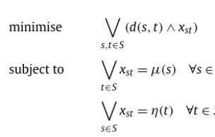
asthevalueofthefollowingmathematicalprogrammingproblem(MP):

minimise

s,t∈S

(

d

(

s

,

t

)

∧

xst

)

(1)

subject to

t∈S

xst

=

μ

(

s

)

∀

s

∈

S (2)

s∈S

xst

=

η

(

t

)

∀

t

∈

S (3)

xst

≥

0

∀

s

,

t

∈

S (4)

Itisshownin[3,Theorem 1] thatforeachd

∈

D

(

S

)

,d

ˆ

isapseudo-ultrametricon

F

(

S

)

.

Definition4.Wedefinetheorder

on

D

(

S

)

as

d1

d2ifd1

(

s

,

t

)

≤

d2

(

s

,

t

)

for alls

,

t

∈

S

.

Apartiallyorderedset

(

X

,

≤

)

isacompletelatticeifeverysubsetof X hasasupremumandaninfimumin

(

X

,

≤

)

.Itcan be easily shownthat

(

D

(

S

),

)

isa completelattice, followingthesameargumentin [3,Lemma2],withthe supremum andinfimumgivenby

_{s,t∈S,d∈D(S)}d

(

s

,

t

)

and

_{s,t∈S,d∈D(S)}d

(

s

,

t

)

.

Definition5.Let

(

X

,

d

)

beapseudo-ultrametricspace.Foranyx

∈

X andY

⊆

X,define

d

(

x

,

Y

)

=

y∈Yd

(

x

,

y

),

ifY

=

∅

1

,

otherwise

Further,givenapairY

,

Z

⊆

X,theHausdorffdistanceinducedbydisdefinedas

Hd

(

Y

,

Z

)

=

0

,

ifY

=

Z

=

∅

y∈Yd

(

y

,

Z

)

∨

z∈Zd

(

z

,

Y

)

,

otherwise

Itisshownin[3,Lemma3] that,ifdisapseudo-ultrametricon X,Hd isapseudo-ultrametricon

P

(

X

)

.

Example3.GivenFig.1,let Y

= {

s1

,

s2

}

⊆

S and Z

= {

s3

,

s4

}

⊆

S. Thedistanced3 is definedasfollows: d3

(

s1

,

s3

)

=

0

.

92,

d3

(

s1

,

s4

)

=

0

.

83,d3

(

s2

,

s3

)

=

0

.

66,d3

(

s2

,

s4

)

=

0

.

75.As a result, d3

(

s1

,

Z

)

=

min

{

d3

(

s1

,

s3

),

d3

(

s1

,

s4

)

}

=

min

{

0

.

92

,

0

.

83

}

=

0

.

83,andd3

(

s2

,

Z

)

=

min

{

d3

(

s2

,

s3

),

d3

(

s2

,

s4

)

}

=

min

{

0

.

66

,

0

.

75

}

=

0

.

66.Meanwhile,d3

(

s3

,

Y

)

=

inf

{

d3

(

s3

,

s1

),

d3

(

s3

,

s2

)

}

=

min

{

0

.

92

,

0

.

66

}

=

0

.

66,andd3

(

s4

,

Y

)

=

min

{

d3

(

s4

,

s1

),

d3

(

s4

,

s2

)

}

=

min

{

0

.

83

,

0

.

75

}

=

0

.

75.TheHausdorffdistanceinduced

byd3isdefinedas

Hd3

(

Y

,

Z

)

=

max

{

d3(s1,Z

),

d3(s2,Z

),

d3(s3,Y

),

d3(s4,Y

)

}

=

max

{

0

.

83

,

0

.

66

,

0

.

66

,

0

.

75

} =

0

.

83

.

2

Note that anyd

∈

D

(

S

)

induces a pseudo-ultrametric d

ˆ

on

F

(

S

)

which, in turn, yields a pseudo-ultrametric H_dˆ on

P

(

F

(

S

))

.Wearenowinapositiontodefineafunctional

on

D

(

S

)

.

Definition6.Thefunctional

γ

:

D

(

S

)

→

D

(

S

)

isdefinedasfollows.Foranyd

∈

D

(

S

)

,

γ

(

d

)

isgivenby

γ

(

d

)(

s

,

t

)

=

γ

·

a∈A

H_dˆ

δ(

s

,

a

), δ(

t

,

a

)

foralls

,

t

∈

S,where

γ

∈

(

0

,

1

]

isthediscountingfactor.

Itisratherstraightforwardtocheckthat

γ

(

d

)

∈

D

(

S

)

by[3,Lemma3],whichmeansthat

γ iswelldefined.Incase

γ

=

1,itisshownin[3,Lemma4] thatthefunctional

1

:

D

(

S

)

→

D

(

S

)

ismonotonicwithrespecttothepartialorder

. One canalso seethat thisholdsaswell in thecasethat

γ

∈

(

0

,

1

)

.ByTarski’s fixpointtheorem [26],

γ admitsa least fixpoint

γ_mingivenby

γ_min

=

{

d

∈

D

(

S

)

|

γ

(

d

)

d

}

.

ThisiswhatweareafterasadistancemeasureonthepairsofstatesinanFTS.Notethat

Definition7.Let

(

S

,

A

,

δ)

beanFTSand

γ

∈

(

0

,

1

]

bethediscountingfactor.Foranys

,

t

∈

S,thebehaviouraldistancebetween sandt,denoteddγ_f

(

s

,

t

)

(f standsforfixpoint),isdefinedas

dγ_f

(

s

,

t

)

=

γ_min

(

s

,

t

).

Remark1.In[3],theorder

isdefinedinthereversedirectionasinDefinition4,i.e.,d1

d2 ifd1

(

s

,

t

)

≥

d2

(

s

,

t

)

.

Accord-ingly,dγ_f isdefinedasthegreatestfixpoint(asopposedtotheleastfixpoint here).Thisisusedtomimicthebisimulation whichiscommonlydefinedasthegreatestfixpointintheliterature.Neverthelessthesetwodefinitionsareequivalent.

Remark2(Discounting).Thetransitionscouldbewrittenass

−→

a

μ

andt

−→

a

η

.Inotherwords,theone-stepsuccessorsof sandt arethedistributions

μ

and

η

.Thedistancebetweensandt iscalculatedbytheHausdorffdistancebetweentheir one-stepsuccessors.Asitisonestepawayfromsandt,thecontributionofthedistancewillbediscountedby

γ

.

3. Polynomialalgorithmsforcomputingdistances

Proposition1.Let

(

S

,

A

,

δ)

beanFTSand

γ

bethediscountingfactor.Define

(

γ

)

0

(

⊥

)

= ⊥

and

(

γ

)

n+1

(

⊥

)

=

γ

[

(

γ

)

n

(

⊥

)

]

, where

⊥

isgivenby

⊥

(

s

,

t

)

=

0foralls

,

t

∈

S.Thendγ_f

=

γ_min

=

{

(

γ

)

n

(

⊥

)

|

n

∈

N

}

.

Proof. By Kleene’sfixpoint theorem, the leastfixpoint

γ_min can be obtainedby iteration of

γ starting fromthe least element

⊥

(see, for example,[10]). As a result, to verify that

γ_min

=

{

(

γ

)

n

(

⊥

)

|

n

∈

N

}

,it suffices to show that the closure ordinalof

γ,i.e., theleast ordinaln such that

(

γ

)

n+1

=

(

γ

)

n, isatmost

ω

.Infact, forany

(

s

,

t

)

∈

S

×

S,if s

−→

a

μ

,then foreachdn

=

(

γ

)

n

(

⊥

)

,thereexists

η

n suchthat t

a

−→

η

n andd

ˆ

n

(

μ

,

η

n

)

≤

dn

(

s

,

t

)

.Because theFTSunder

the complexity consideration is finite, which means that

δ(

t

,

a

)

is finite, there is an

η

n, say

η

, such that t a

−→

η

and

ˆ

dn

(

μ

,

η

)

≤

dn

(

s

,

t

)

forallbutfinitelymanyn,asdesired.

2

AsmentionedinSection1,Proposition1doesnotyieldanoutrightpolynomial-timealgorithm.Forourpurpose, essen-tiallyonehastoshowthat

(1) the(non-standard)mathematicalprogramming(MP)problemcanbesolvedinpolynomialtime;and (2) itonlyrequirespolynomiallymanyiterationstoreachthefixpoint.

In thesequel,wewillshow bothareindeedthecase. For(1),weshallpresentapolynomial-timealgorithmthat,givend ands

,

t

∈

S,computes

γ

(

d

)(

s

,

t

)

=

γ

·

a∈A

H_dˆ

(δ(

s

,

a

), δ(

t

,

a

)).

Intuitively,

γ

(

d

)(

s

,

t

)

isthenewdistance ofs andt afterapplying thefunctional

γ tofunction d(oneiteration). This suffices toshow thateach iteration

γ can bedone inpolynomial timeineithercase. For(2)it turnsout thatthe non-discountedanddiscountedcasedemanddifferentargumentswhichwewillprovideinSection4andSection5,respectively.

4. Thenon-discountedcase

Inthissection,we considerthenon-discountedcase,i.e.,

γ

=

1.We omitthesuperscript1of

1 andsimply write

instead.

4.1. TheconstructionofanMPproblem

Westartwithsomesimpleobservations.Givenany

M

,wewrite _M tobe

{

μ

(

s

)

|

s

∈

S

,

μ

∈

F

(

S

)

} ∪ {

0

,

1

}

.

Clearly

|

_M

|

≤ |

M

|

.Intuitively, _M isthesetofvaluesappearingin

M

asdegreesofmembershipaswellas0 and1.

Example4.GiventheFTS

M

inFig.1, _M

= {

0

,

0

.

6

,

0

.

8

,

0

.

9

,

1

}

.

2

Thefollowinglemmahasbeenimpliedin[5,p. 738,Remark 1] andisratherstraightforward.Hencetheproofisomitted.

Lemma1.Let

(

d

)(

s

,

t

)

=

_a∈AH_dˆ

(δ(

s

,

a

),

δ(

t

,

a

))

,foranys

,

t

∈

S.Itholdsthat

(

d

)(

s

,

t

)

∈

_M

∪ {

d

(

s

,

t

)

|

s

,

t

∈

S

}

.

Wenote thatthisobservationdoesnot holdinthediscountedcase. Owningtothisobservation, tocalculate

(

d

)(

s

,

t

)

, we onlyneedtotestwhethereachmemberof _M

∪ {

d

(

s

,

t

)

|

s

,

t

∈

S

}

canbe attainedandtheleastattainedvalue isthe sought one. Hence we can reduce the optimisation problemto the feasibility testingof a systemof equations

of the followingform:

⎧

⎪

⎪

⎪

⎪

⎨

⎪

⎪

⎪

⎪

⎩

1≤i,j≤n

(

di j

∧

xi j

)

=

c

(

∗

)

x11

∨

x12

· · · ∨

x1k1

=

a1

..

.

xm1

∨

xm2

· · · ∨

xmkm

=

am

,

wherec

∈

_M

∪ {

d

(

s

,

t

)

|

s

,

t

∈

S

}

.Tothisend,wefirstrewriteEq.

(

∗

)

as

∨

Y

=

c

,

whereY

= {

xi j

|

di j

≥

c

}

,

(

∗∗

)

⎧

⎪

⎪

⎪

⎪

⎨

⎪

⎪

⎪

⎪

⎩

∨

Y

=

c

,

whereY

= {

xi j

|

di j

≥

c

}

x11

∨

x12

· · · ∨

x1k1

=

a1

..

.

xm1

∨

xm2

· · · ∨

xmkm

=

am

(5)

BelowweleveragetheexampleFTSinFig.1toillustratetheconstruction.

Example5.Recallthathere

μ

=

0.9 s3

+

0.8

s4 and

η

=

0.6

s3

+

0.9

s4.Inthisexample,weshow givend1 suchthat d1

(

i

,

i

)

=

0 for all i

∈ {

1

,

..,

4

}

andd1

(

i

,

j

)

=

1 for all i

=

j and i

,

j

∈ {

1

,

...,

4

}

.Here, M

∪ {

d

(

s

,

t

)

|

s

,

t

∈

S

}

= {

0

,

0

.

6

,

0

.

8

,

0

.

9

,

1

}

.In this

example,wepickc

=

0

.

6,andthesystem

ofequationsisasfollows:

⎧

⎪

⎪

⎪

⎪

⎪

⎪

⎪

⎪

⎪

⎪

⎪

⎪

⎪

⎪

⎪

⎨

⎪

⎪

⎪

⎪

⎪

⎪

⎪

⎪

⎪

⎪

⎪

⎪

⎪

⎪

⎪

⎩

i=jxi j

=

c

=

0

.

6

x11

∨

x12

∨

x13

∨

x14

=

0

μ

(

s1)

=

0 x21

∨

x22

∨

x23

∨

x24

=

0

μ

(

s2)

=

0 x31

∨

x32

∨

x33

∨

x34

=

0

.

9

μ

(

s3)

=

0

.

9 x41

∨

x42

∨

x43

∨

x44

=

0

.

8

μ

(

s4)

=

0

.

8 x11

∨

x21

∨

x31

∨

x41

=

0

η

(

s1)

=

0 x12

∨

x22

∨

x32

∨

x42

=

0

η

(

s2)

=

0 x13

∨

x23

∨

x33

∨

x43

=

0

.

6

η

(

s3)

=

0

.

6 x14

∨

x24

∨

x34

∨

x44

=

0

.

9

η

(

s4)

=

0

.

9

(6)

Notethatsystemsofequationsforothervaluesofccanbeconstructedinthesameway.

2

4.2. Checkingfeasibility

Recallthatnowwehaveasystemofequations

(whichcanberewrittenas

).Ourtaskistocheckwhetherboth

and

arefeasible,i.e.,whetherthereexistsasolutiontomake

and

hold.

Lemma2.

isfeasibleiff

isfeasible.

Proof. Itis toshow that

(

∗

)

and

(

∗∗

)

are equivalent. Werewrite

(

∗

)

assup1≤i,j≤n

{

(

di j

∧

xi j

)

}

=

c. Forall 1

≤

i

,

j

≤

n, if

di j

<

c,thendi j

∧

xi j

<

c.Asaresult,this

(

di j

∧

xi j

)

isnotcontributingtosup1≤i,j≤n

{

(

di j

∧

xi j

)

}

=

c andcanberemoved.

2

GivenLemma2,itremainstoshowhowtocheckthefeasibilityofasystemofequations

oftheform

⎧

⎪

⎪

⎨

⎪

⎪

⎩

x11

∨

x12

· · · ∨

x1k1

=

a1

..

.

xm1

∨

xm2

· · · ∨

xmkm

=

am

Forthispurpose,weconstructavaluationforxi (1

≤

i

≤

n)as

xi

=

min

{

a

|

ais the RHS of an equation

π

of

s.t.xi,joccurs in

π

}

Thefollowinglemmaplaysavitalrole.Inother words,inordertocheckthefeasibilityof

,itsufficestocheckwhether

x

=

(

xi

)

1≤i≤n isasolutionof

.Thiscanbedoneinlineartime. Lemma3.

isfeasibleiff

x

=

(

xi

)

1≤i≤nisasolutionof

.

Proof. The“if”partisobviousandwewillfocuson the“onlyif”part.Fixany1

≤

i

≤

m.Bythedefinitionof

x,we have that, foreach 1

≤

j

≤

ki, xi j

=

min

{

a

|

xh

=

xi j for some 1

≤

h

≤

k

}

.Clearly ai

∈ {

a

|

xh

=

xi j for some 1

≤

h

≤

k

}

,and thuswehavethatxi j

≤

ai.Itfollowsthat

xi1

∨

xi2

· · · ∨

xiki

≤

ai

.

Since

is feasible,theremustexista solutionx

of

.Foreach 1

≤

i

≤

n,xi

≤

a withxh

=

xi forsome1

≤

h

≤

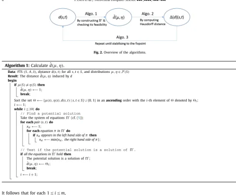
k. Consequently

[image:9.561.39.519.40.436.2]

Fig. 2.Overview of the algorithms.

Algorithm 1:Calculated

ˆ

(

μ

,

η

)

.

Data: FTS(S,A,δ),distanced(s,t)foralls,t∈S,anddistributionsμ,η∈F(S)

Result: Thedistancedˆ(μ,η)inducedbyd begin

ifμ(S)=η(S)then

ˆ

d(μ,η)←−1; break;

Sorttheset ←− {μ(s),η(s),d(s,t)|s,t∈S}∪ {0,1}inanascendingorderwiththei-thelementof denotedby i;

i←−1; whilei≤ | |do

// Find a potential solution Takethesystemofequations(cf. (5)); for eachpair(s,t)do

xst←−1;

for eachequationπindo

ifxstappearsinthelefthandsideofπthen

xst←−min{xst,the right hand side ofπ};

// Test if the potential solution is a solution of . ifalltheequationsinholdthen

Thepotentialsolutionisasolutionof;

ˆ

d(μ,η)←− i;

break;

i←−i+1;

Itfollowsthatforeach1

≤

i

≤

m,

ai

=

xi1

∨

xi2

· · · ∨

xik1

≤

xi1

∨

xi2

· · · ∨

xik1

≤

ai Namely,

xisasolutionof

.

2

4.3. Thealgorithms

Based ontheresultsinSection 4.1and4.2,wespecifythreealgorithmshere.As illustratedinFig.2,giventhecurrent d

(

s

,

t

)

Algorithm1computesd

ˆ

(

μ

,

η

)

.TheresultsactastheinputforAlgorithm2,whichcalculatestheupdatedd

(

s

,

t

)

,i.e.,

(

d

)(

s

,

t

)

.InAlgorithm3,itrepeatstheprocedureuntilafixpointisreached.

WewillcontinuewithExample5toshowhowtocalculated

ˆ

1

(

μ

,

η

)

.

Example6(Continued).According to the algorithm,

= {

0

,

0

.

6

,

0

.

8

,

0

.

9

}

. The algorithm will start from 1

=

0. It turns

out thisis not a feasible solution.We will proceed to check 2

=

0

.

6. As a result, we obtain a potential solution x33

=

min

{

0

.

9

,

0

.

6

}

=

0

.

6,x34

=

min

{

0

.

6

,

0

.

9

,

0

.

9

}

=

0

.

9,x44

=

min

{

0

.

8

,

0

.

9

}

=

0

.

8,x43

=

min

{

0

.

6

,

0

.

8

,

0

.

6

}

=

0

.

6 andxi j

=

0 forall

therestvariablesxi j.

Now wetestwhetherthepotential solutionisreallyasolutionof

inEq. (6).Thisisdonebysubstitutingthevalues backtoEq. (6).Itisclearthatx31

∨

x32

∨

x33

∨

x34

=

0

.

9,but0

∨

0

∨

0

.

6

∨

0

.

6

=

0

.

6

=

0

.

9.Sothispotentialsolutionisnota

solutionof

.

The algorithm proceedsby checkingthe next candidate 3

=

0

.

8, whichturns out not to be a solution of

either.

It thenchecks 4

=

0

.

9.Here,we havex33

=

min

{

0

.

9

,

0

.

6

}

=

0

.

6, x34

=

min

{

0

.

9

,

0

.

9

,

0

.

9

}

=

0

.

9, x44

=

min

{

0

.

8

,

0

.

9

}

=

0

.

8,

x43

=

min

{

0

.

9

,

0

.

8

,

0

.

6

}

=

0

.

6 andalltherestxi j

=

0.Thispotential solutionis indeedasolutionof

.Wethenconclude

thatthedistancebetween

μ

and

η

inducedbyd1 isd

ˆ

1

(

μ

,

η

)

=

0

.

9.

2

Algorithm 2:Calculate

(

d

)(

s

,

t

)

.

Data: FTS(S,A,δ),ands,t∈S,distancefunctiond Result:(d)(s,t)

begin

ifAct(s)=Act(t)then(d)(s,t)=1; else

//computeHausdorffdistancebycallingAlgo.1

Hdˆ(δ(s,a), δ(t,a))=

η∈δ(t,a)μ∈δ(s,a)

ˆ

d(μ,η) μ∈δ(s,a)η∈δ(t,a)

ˆ

d(μ,η);

//compute(d)(s,t)bytakingthesupremumamongallactions:

(d)(s,t)=a∈Act(s)Hdˆ(δ(s,a),δ(t,a));

Lemma2andLemma3giveriseto:

Proposition2.Algorithm2computes,foreachd,

(

d

)

inpolynomialtime.

We remark that this is actually a strongly polynomial-time algorithm. In the literature, strongly polynomial time is definedinthearithmeticmodelofcomputation.Inthismodel,thebasicarithmeticoperations(addition,subtraction, multi-plication,division,andcomparison)takeaunittimesteptoperform,regardlessofthesizesoftheoperands.Thealgorithm runsinstronglypolynomialtime [20] if(1) thenumberofarithmeticoperationsisboundedbyapolynomial in

|

M

|

;and (2) thespaceusedbythealgorithmisboundedbyapolynomialin

||

M

||

.Inourcase,onecaneasilyverify(1)and(2)hold forAlgorithm2.

Algorithm 3 is the main procedure to compute d1_f

(

s

,

t

)

by an iteration of

starting from the leastelement

⊥

. The correctness ofthe algorithm follows fromProposition 2, whichalso asserts that each iteration requires polynomial time only.Henceitsufficestoshowthatonlypolynomialnumberofiterationsarenecessarytoterminatethealgorithm.

Algorithm 3:Calculated1_f.

Data: FTS(S,A,δ)

Result: Thebehaviouraldistancematrixd1 f

begin n←−0; d0←− ⊥; repeat

Dl←−dn;

for eachpair(s,t)do

dn+1(s,t)←−(dn)(s,t);// Call Algo. 2

D←−dn+1;

n←−n+1; until Dl=D;

d1 f=D;

ThefollowinglemmacanbeobtainedbyinductionandLemma1.

Lemma4.Given

M

=

(

S

,

A

,

δ)

,itholdsthatd1

f

(

s

,

t

)

∈

Mforanys

,

t

∈

S.

Thefollowingpropositionshowsonlypolynomialnumberofiterationsarenecessarytoterminatethealgorithm.

Proposition3.TheiterationinAlgorithm3needsatmostpolynomiallymanysteps.

Proof. We assume that n

∈

N

is the smallest n such that dn

(

s

,

t

)

=

dn+1

(

s

,

t

)

. Due to Lemma 4, di

(

s

,

t

)

∈

M, for any

i

∈ [

0

,

n

]

.Notethat eachdi isofdimension

|

S

|

2,andthus thevalueofeach entrydst mustbein _M.Moreover,as

is

monotonic,di+1

≤

di.Itfollowsthatn

≤ |

_M

|

· |

S

|

2,whichispolynomialinthesizeof

M

.

2

Weconcludethissectionbythefollowingtheorem,whichcanbeeasilyshownbyProposition2and3.

Theorem1.Givenafuzzytransitionsystem

M

,andtwostatess

,

t,d1

5. Thediscountedcase

Inthissection,weconsiderthediscountedcase,i.e.,

γ

<

1.Firstweremarkthatonecannot(atleastnotina straight-forward manner) follow the same approach asin Proposition 3 to obtain a polynomial-time algorithm, simply because Lemma 4failswhen

γ

<

1.Instead, ourstrategy is tofirst comeup withan approximation algorithm, which,givenany

>

0,computesadsuchthat

||

d

−

dγ_f

||

≤

.Itturnsoutthatsuchanapproximationcanbeidentifiedbyapplyingatmost

log_γ

iterations.Inthesequel,weconsiderthe

∞

-normforvectors,i.e.,

||

d1

−

d2

||

=

maxs,t∈S

|

d1

(

s

,

t

)

−

d2

(

s

,

t

)

|

.Wefirst

showthat

isacontractionmapping.Thefollowingisasimpletechnicalfact.

Lemma5.Foranyz1

,

z2

,

t

∈

R

,itholdsthatmin

(

z1

,

t

)

−

min

(

z2

,

t

)

≤ |

z1

−

z2

|

.

Proof. Observethatmin

(

z

,

t

)

=

|

z

+

t

| − |

z

−

t

|

2 .Itthenfollowsthat min

(

z1,t

)

−

min

(

z2,t

)

=

|

z1

+

t

| − |

z1

−

t

| + |

z2

−

t

| − |

z2

+

t

|

2

≤

|

(

z2

−

t

)

−

(

z1

−

t

)

| + |

(

z1

+

t

)

−

(

z2

−

t

)

|

2

= |

z1

−

z2

|

.

2

Forsimplicity,given

μ

and

η

,wewriteUμ,ηforthesetof

{

xuv

}

u,v∈S suchthat

⎧

⎪

⎨

⎪

⎩

v∈Sxuv

=

μ

(

u

)

∀

u

∈

S

u∈Sxuv

=

η

(

v

)

∀

v

∈

S

xuv

≥

0

∀

u

,

v

∈

S

Lemma6.Foranyd

,

d

:

S

×

S

→ [

0

,

1

]

,itholdsthat

||

γ

(

d

)

−

γ

(

d

)

|| ≤

γ

· ||

d

−

d

||

.

Proof. Bydefinition,

||

γ

(

d

)

−

γ

(

d

)

|| =

max

s,t∈S

|

γ

₍

_d

₎₍

_s

_,

_t

₎

₋

γ

₍

_d

₎₍

_s

_,

_t

₎

_|

_.

Fixtwostatessandt.Wehavethefollowing:

|

γ

(

d

)(

s

,

t

)

−

γ

(

d

)(

s

,

t

)

|

= |

γ

·

a∈A

H_dˆ

(δ(

s

,

a

), δ(

t

,

a

))

−

γ

·

a∈A

Hd

(δ(

s

,

a

), δ(

t

,

a

))

|

≤

γ

· |

H_dˆ

(δ(

s

,

a∗

), δ(

t

,

a∗

))

−

Hd

(δ(

s

,

a∗

), δ(

t

,

a∗

))

|

[

wherea∗

=

arg max

a∈A Hdˆ

(δ(

s

,

a

), δ(

t

,

a

))

]

≤

γ

· |ˆ

d

(

μ

∗

,

η

∗

)

− ˆ

d

(

μ

∗

,

η

∗

)

|

[

where

(

μ

∗

,

η

∗

)

=

argH_dˆ

(δ(

s

,

a∗

), δ(

t

,

a∗

))

]

=

γ

· |

min

x∈Uμ∗,η∗

u,v∈S

(

d

(

u

,

v

)

∧

xuv

)

−

min

x∈Uμ∗,η∗

u,v∈S

(

d

(

u

,

v

)

∧

xuv

)

|

≤

γ

· |

u,v∈S

(

d

(

u

,

v

)

∧

yuv

)

−

u,v∈S

(

d

(

u

,

v

)

∧

yuv

)

|

[

where

y

=

arg min

x∈Uμ∗,η∗

u,v∈S

(

d

(

u

,

v

)

∧

xuv

)

]

≤

γ

· |

d

(

u∗

,

v∗

)

∧

yu∗v∗

−

d

(

u∗

,

v∗

)

∧

yu∗v∗

|

[

where

(

u∗

,

v∗

)

=

arg max

≤

γ

· |

d

(

u∗

,

v∗

)

−

d

(

u∗

,

v∗

)

| [

By Lemma5

]

≤

γ

· ||

d

−

d

||

Namely,foranys

,

t

∈

S,

|

γ

(

d

)(

s

,

t

)

−

γ

(

d

)(

s

,

t

)

| ≤

γ

· ||

d

−

d

||

.

Asaresult,

||

γ

(

d

)

−

γ

(

d

)

|| =

max

s,t∈S

|

γ

₍

_d

₎₍

_s

_,

_t

₎

₋

γ

₍

_d

₎₍

_s

_,

_t

₎

_{| ≤}

_γ

_{· ||}

_d

₋

_d

_||

_.

₂

Lemma6revealsthat

γ isacontractionmapping,hencebytheBanachfixpointtheorem[1],dγ_f isnotonlytheleast, butalsotheuniquefixpointof

γ.

Corollary1.GivenanyFTS

M

withdiscountingfactor

γ

∈

(

0

,

1

)

,letN

=

_loglog_γ

.Then

||

(

γ

)

N

(

d0

)

−

dγ_f

||

≤

.

Proof. First,observethat

||

γ

(

d

)

−

dγ_f

||

≤

γ

· ||

d

−

dγ_f

||

,whichfollowsfromLemma6andthefactthat

γ

(

dγ_f

)

=

dγ_f. Byinduction,wehave

||

(

γ

)

n

(

d0)

−

dγ_f

|| ≤

γ

n

· ||

d0

−

dγ_f

||

.

Hence

||

(

γ

)

N

(

d0

)

−

dγf

|| ≤

γ

N

· ||

d0

−

dγf

|| ≤

γ

N

≤

.

2

Algorithm 4:Calculatedγ_f.

Data: FTS(S,A,δ),errorbound,discountingfactorγ Result: Theapproximatebehaviouraldistancedγ_f begin

N←− loglogr;

d0←− ⊥;

n←−0; repeat

for eachpair(s,t)do

dn+1(s,t)←−γ·(dn)(s,t);// Call Algo.2

D←−dn+1;

n←−n+1; untiln>N; dγf=D;

Corollary 1 states that

(

γ

)

N

(

d0

)

approximates dγ_f up to

. This result is essentially a corollary of Banach fixpoint

theorem.Italsogivesastronglypolynomialapproximation algorithmuptoanyprecision

,asshowninAlgorithm4.This isalmostsufficientforpracticalconsiderations. Theoreticallyappealing,bythestandardcontinuedfractionalgorithm[20], wecancomputetheexact dγ_f inpolynomialtimeaswell.Forthispurpose,weneedthefollowinglemma:

Lemma7.For

γ

∈

(

0

,

1

)

,dγ_f isarationalvectorofsizepolynomialin

||

M

||

and

||

γ

||

.

Proof. Forsimplicitywewritedfordγ_f.Bydefinition,dmustsatisfy

d

(

s

,

t

)

=

γ

· ˆ

d

(

μ

,

η

)

forsomea

∈

A,

μ

∈

δ(

s

,

a

)

,and

η

∈

δ(

t

,

a

)

.Namely

d

(

s

,

t

)

=

γ

·

u,v∈S

(

d

(

u

,

v

)

∧

xu,v

)

⎧

⎪

⎨

⎪

⎩

v∈Sxuv

=

μ

(

u

)

∀

u

∈

S

u∈Sxuv

=

η

(

v

)

∀

v

∈

S xuv

≥

0

∀

u

,

v

∈

S

Theclaimhencefollowsfrombasiclinearalgebra.

2

Theorem2.Forafixed

γ

,d canbecomputedexactlyinpolynomialtimein

||

M

||

.

Proof. ByTheorem1,wecanfinddγ_f inpolynomialtimein

M

and

avectorthatis

-closetodγ_f.AndbyLemma7,dγ_f isarationalvectorofsizepolynomialin

M

.Sowecanusethecontinuedfractionalgorithm[20,Chapter 5] tocompute dinpolynomialtime,asisillustratedin[6].

2

We remark that, unfortunately,the exact polynomial-timealgorithm isnot strongly polynomial,as continuedfraction algorithmisused.Itisanopen questionwhetheronecanobtainanexactstronglypolynomial-timealgorithm.Asafuture work,wewouldimplementthealgorithmsandprovideexperimentalresultstoshowiftheyworkwellinpractice.

6. Conclusion

Wehavestudiedthealgorithmicaspectofbehaviouraldistanceforfuzzytransitionsystems.Thepseudo-ultrametric de-finedin[5] wasextendedtoaccommodateboththediscountedandnon-discountedsettings.Wethenprovided polynomial-timealgorithmstocalculatethebehaviouraldistanceinbothcases.

Acknowledgements

TaolueChenispartiallysupportedbyEPSRCgrant(EP/P00430X/1),ARCDiscoveryProject(DP160101652,DP180100691), andtheNationalNaturalScienceFoundation ofChina(GrantNo. 61662035).TingtingHanispartiallysupportedbyEPSRC grant(EP/P015387/1).YongzhiCaoissupportedbyNationalNaturalScienceFoundationofChina(GrantNo.61772035and 61751210).

References

[1]S.Banach,Surlesopérationsdanslesensemblesabstraitsetleurapplicationauxéquationsintégrales,Fund.Math.3(1922)133–181. [2]P.Buchholz,Bisimulationrelationsforweightedautomata,Theoret.Comput.Sci.393 (1–3)(2008)109–123.

[3]Y.Cao,G.Chen,E.E.Kerre,Bisimulationsforfuzzy-transitionsystems,IEEETrans.FuzzySyst.19 (3)(2011)540–552. [4]Y.Cao,Y.Ezawa,Nondeterministicfuzzyautomata,Inform.Sci.191(2012)86–97.

[5]Y.Cao,S.X.Sun,H.Wang,G.Chen,Abehavioraldistanceforfuzzy-transitionsystems,IEEETrans.FuzzySyst.21 (4)(2013)735–747.

[6]D.Chen,F.vanBreugel, J.Worrell,Onthe complexityofcomputingprobabilisticbisimilarity,in:L. Birkedal(Ed.),FoSSaCS,in:LectureNotesin ComputerScience,vol. 7213,Springer,2012,pp. 437–451.

[7]T.Chen,T.Han,J.Lu,Onmetricsforprobabilisticsystems:definitionsandalgorithms,Comput.Math.Appl.57 (6)(2009)991–999. [8]M.´Ciri´c,J.Ignjatovi ´c,N.Damljanovi ´c,M.Baši ´c,Bisimulationsforfuzzyautomata,FuzzySetsandSystems186 (1)(2012)100–139.

[9]M. ´Ciri´c,J.Ignjatovi ´c,I.Janˇci ´c,N.Damljanovi ´c,Computationofthegreatestsimulationsandbisimulationsbetweenfuzzyautomata,FuzzySetsand Systems208(2012)22–42.

[10]B.Davey,H.Priestley,IntroductiontoLatticesandOrder,CambridgeMathematicalTextBooks,CambridgeUniversityPress,2002.

[11]L.deAlfaro,T.A.Henzinger,R.Majumdar,Discountingthefutureinsystemstheory,in:J.C.M.Baeten,J.K.Lenstra,J.Parrow,G.J.Woeginger(Eds.),ICALP, in:LectureNotesinComputerScience,vol. 2719,Springer,2003,pp. 1022–1037.

[12]W.Deng,D.Qiu,Supervisorycontroloffuzzydiscrete-eventsystemsforsimulationequivalence,IEEETrans.FuzzySyst.23 (1)(Feb2015)178–192. [13]Y.Deng,T.Chothia,C.Palamidessi,J.Pang,Metricsforaction-labelledquantitativetransitionsystems,Electron.NotesTheor.Comput.Sci.153 (2)

(2006)79–96.

[14]Y. Deng,H. Wu,Modalcharacterisationsofprobabilisticand fuzzybisimulations,in:FormalMethodsand SoftwareEngineering,Springer, 2014, pp. 123–138.

[15]J.Desharnais,V.Gupta,R.Jagadeesan,P.Panangaden,MetricsforlabelledMarkov processes,Theoret.Comput.Sci.318 (3)(2004)323–354. [16]J.Desharnais,R.Jagadeesan,V.Gupta,P.Panangaden,Themetricanalogueofweakbisimulationforprobabilisticprocesses,in:LICS,IEEEComputer

Society,2002,pp. 413–422.

[17]N.Ferns,P.Panangaden,D.Precup,BisimulationmetricsforcontinuousMarkov decisionprocesses,SIAMJ.Comput.40 (6)(2011)1662–1714. [18]H.Fu,ComputinggamemetricsonMarkov decisionprocesses,in:A.Czumaj,K.Mehlhorn,A.M.Pitts,R.Wattenhofer(Eds.),ICALP(2),in:Lecture

NotesinComputerScience,vol. 7392,Springer,2012,pp. 227–238.

[19]A.Giacalone,C.-C.Jou,S.A.Smolka,Algebraicreasoningforprobabilisticconcurrentsystems,in:Proc.ofIFIPWG2.2/2.3,PCM’90,1990,pp. 453–459. [20]M.Grotschel,L.Lovasz,A.Schrijver,GeometricAlgorithmsandCombinatorialOptimization,AlgorithmsandCombinatorics,Springer-Verlag,1993. [21]I.Janˇci ´c,Weakbisimulationsforfuzzyautomata,FuzzySetsandSystems249(2014)49–72.

[22]S.C.Kleene,IntroductiontoMetamathematics,North-Holland,1952. [23]R.Milner,CommunicationandConcurrency,PrenticeHall,1989.

[24]H.Pan,Y.Li,Y.Cao,Lattice-valuedsimulationsforquantitativetransitionsystems,Internat.J.Approx.Reason.56(2015)28–42. [25]R.T.Rockafellar,R.J.-B.Wets,VariationalAnalysis,Springer-Verlag,2005.

[26]A.Tarski,Alattice-theoreticalfixpointtheoremanditsapplications,PacificJ.Math.5(1955)285–309.

[28]F.vanBreugel,B.Sharma,J.Worrell,Approximatingabehaviouralpseudometricwithoutdiscountforprobabilisticsystems,Log.MethodsComput.Sci. 4 (2)(2008).

[29]F.vanBreugel,J.Worrell,Analgorithmforquantitativeverificationofprobabilistictransitionsystems,in:K.G.Larsen,M.Nielsen(Eds.),CONCUR,in: LectureNotesinComputerScience,vol. 2154,Springer,2001,pp. 336–350.

[30]F.vanBreugel,J.Worrell,Abehaviouralpseudometricforprobabilistictransitionsystems,Theoret.Comput.Sci.331 (1)(2005)115–142.