New Algorithm - Simulation Connected Components Labeling for Binary Images.

(1)

International Journal of Emerging Technology and Advanced Engineering

Website: www.ijetae.com (ISSN 2250-2459, ISO 9001:2008 Certified Journal, Volume 3, Issue 12, December 2013)

335

New Algorithm - Simulation Connected Components

Labeling for Binary Images.

Yahia S. Halabi

Prof. of Computer Science, Princess Sumaya University for Information Technology, Amman-Jordan [email protected]

Abstract— This research presents an algorithm for labeling

connected components in binary images based on searching around black operations of an image. The proposed new algorithm walks around black to identify their boundaries. A one-dimensional array used to keep label equivalences, for uniting equivalent labels successively during the operations in different directions. The boundaries of the object are the most interesting parts to be identified. The algorithm applies two processes of labeling, one is row-wise from left to right and one is column-wise, from top to bottom at initial zero iteration. A sub image I[I,J] i+1 , is defined after each labeling allocation. It is generated by subtracting the iterative labeling obtained at I [I, J]i row-wise and labeling obtained at I[I,J]i column-wise. The new image for next iteration I[I,J]i+1= I[I,J] i - (labeling obtained from image I[I,J]i row-wise ∩ labeling obtained from image I[I,J]i column-wise) . The proposed algorithm is very useful in different areas of image processing such as, medical imaging which focus on accuracy than other important measurements as well. One important application is the medical image that shows a tumor surrounded by other part of body such as bones, lungs and others. It has been shown that the efficiency of the proposed algorithm is comparative to those of the conventional algorithms. The data structure used is the stack and the stack operations are its main engine. The data pushed or popped to or from the stack, presents the directions to be taken in consideration for searching, in order to determine the boundary pixels, to detect the connected components iteratively. It is found that the execution time of the proposed algorithm is proportional to the number of pixels in connected components of an image. The proposed algorithm can also be used and generalized for higher dimensions. The proposed algorithm has desirable characteristics in term of accuracy with acceptable CPU computer time. Such method based on walking around black, to mark their boundaries.

Keywords:Binary Image, Binary mask. Connected Components, Stack, Push and Pop operation.

I. INTRODUCTION

Connected components labeling, scans an image and

groups its pixels into components based on pixel connectivity, i.e. all pixels in a connected component, share similar pixel intensity values, and are in some way connected with each other. It is commonly used to refer to the task of grouping the connected pixels in an image.

Extracting and labeling of various disjoint and connected components in an image, is central to many automated image analysis applications. Mathematical formulation of the problem can also be written as follows:

A graph G=(N, E) can be thought of as a collection of points (here-after nodes) N={i, i=1..n}, where n=|N| is the number of nodes, connected via directed or undirected links (arcs), E={e(i, j) for some i and j in N}, where m=|E| is the number of arcs in the graph and e(i, j) denotes an arc whose head is i and tail is j. We can represent a graph efficiently by specifying n and m and giving an array A(m,2) giving the heads and tails of each arc:

A(e(i,j),:)=[i,j] ………….(1)

(2)

International Journal of Emerging Technology and Advanced Engineering

336 However, there are several labels in the region of corresponding component in binary mask to merge these regions in labeled image and give them a single label for each object. The operation of merge building segment labels, are part of a building object indeed. They found that the traversing of the pixels of objects in the binary mask is the most cumbersome way.

[image:2.612.329.557.407.585.2]

Other algorithms where developed in this field by [2,3,5,10]. They developed new strategies that can be used to improve the speed of connected component labeling algorithms. To assign a label to a new object, most labeling algorithms use a scanning step that examines some of its neighbors. One strategy exploits the dependencies among the neighbors to reduce the number of neighbors examined. Second strategy uses an array to store the equivalence information among the labels. This algorithm replaces the pointer based rooted trees used to store the same equivalence information. It reduces the memory required and also produces consecutive final labels and array based structure instead of the pointer. Such continuous development shows that after completing the scan, the equivalent label pairs, are sorted into equivalence classes and a unique label is assigned to each class. The proposed algorithm were very useful in different interesting areas of image processing such as, medical imaging related to a tumor surrounded by other part of body such as bones, lungs and others. In an early version containing only empirical study of the algorithms were reported at SPIE Medical Imaging Conference 2005 and others [10]. Actual and practical images were not included in most of the algorithms showing its validity for different binary images. Key element of their algorithms were based on a simple union-find data structure and a set of algorithm to work on it [7,9,11 ].

Two linear-time algorithms on this topics is presented by [7], the first also for reporting the number of connected components and the other for labeling every element of value 1 (or white pixel) by its component index. An important feature of their input image algorithms is that they can be implemented without using any extra array other than the one, or and they are suitable for embedded

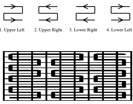
software. [3,4], developed a generalization of polygons by showing explicit mapping between the first non-negative integers and the n-sequentially traversed vertices of any of Peano polygons. Such generalized polygons have been later called Murray polygons, since they are derived using multiple radix or Murray arithmetic [3,5]. It has been noticed also that Murray polygons divided an image into a collection of tiles or run- lengths of different sizes and shapes. Hence, the pixels which are lying inside a tile need not be considered for finding the connected components. Also, for the points which are on the boundary of a tile, one needs to consider connectivity in at most three directions instead of eight directions, taking in consideration an efficient algorithm for: Curve direction (the start point of curve in a tile), boundary pixels detecting (different cases which determine the size of a tile) and direction number (the neighborhood points which have to be considered for the boundary points, connected labeling must be numbered according to the 8-neighbour direction). Such considerations are shown in Figure 1.

1. Upper Left 2. Upper Right 3. Lower Right 4. Lower Left

Figure 1. Curve directions.

(3)

International Journal of Emerging Technology and Advanced Engineering

337 Applying boundary pixels procedure as described before requires visiting each pixel in the tile and consequently visiting all pixels in the binary image. This results to a waste of large computer time for unnecessary visit of large number of pixels, in order to determine which one is inner and which is boundary.

Polygons deal with a tile to be completely black or white, depending upon an accuracy parameter input by user. This means: if the accuracy is 10% then it is enough to make the whole tile black. This makes technique not efficient enough to determine the exact boundary of a tumor region as an example.

For these reasons, we developed a new algorithm which overcomes all the previous difficulties in order to end up with an efficient, fast and accurate result.

II. PREVIOUS KNOWLEDGE AND BASICS OF

MATHEMATICAL STRUCTURE:

A graph G=(N, E) can be thought of as a collection of points (nodes or vertices), N={i, i=1..n}, where n=|N| is the number of nodes, connected via directed or undirected links (arcs), E={e(i, j) for some i and j in N}, and |E| = m which is the number of arcs in the graph and e(i, j) denotes an arc whose head is i and tail is j.

In labeling techniques, we put a label a (number) on each vertex, and doing so creates a label for each edge. Final stage is to label graphs or sub-graph according to various rules, and ask questions about whether the graph can be labeled according to the rules, what the largest number needed as a label might be, how such labels are connected and what are their components. For an N X M size binary image, we use p(x; y) to denote the pixel as well as its value at (x, y) in the image, where 0 <= x < N and 0 <= y < M. We assume that the foreground pixels and background pixels in a given binary image are represented by 1 and 0, respectively. As in most labeling algorithms, we assume that all pixels on the border of an image are background pixels. Connected component labelling works by scanning an image, pixel-by-pixel (from top to bottom

and left to right) in order to identify connected pixel regions, i.e. regions of adjacent pixels which share the same set of intensity values. When only the four nearest neighbours are considered part of the neighbourhood, then pixels p and q are said to be “4-connected When the 8 nearest neighbours are considered part of the neighbourhood, then pixels p and q are said to be “8-connected”. A pixel is a 4-neighbor of pixel p(x, y) if it shares an edge with p(x, y). The 4-neighbors of pixel p(x, y), namely p2, p4, p6 and p8, are shown in Figure 2. On the other hand, a pixel is an 8-neighbor of pixel p(x, y) if it shares an edge or a vertex with p(x, y). The 8-neighbors of pixel p(x, y), namely p1 to p8 are as shown in Figure 3.

[image:3.612.373.472.320.378.2]

Figure 2. The 4-neighbors of pixel p(x, y), namely p2, p4, p6 and p8

Figure 3. The 8-neighbors of pixel p(x, y), namely p1 to p8.

Using the basic general problem statement in most of literature [8], and taking in consideration that the graph G be n × n binary image such that each pixel value G(x, y) is either 0 or 1, then a pixel of value 1 (resp., 0) is called a white pixel (resp., black pixel). For a pixel p(x, y), we define the neighborhoods:

N4(p) = N4(x, y) = {(x, y), (x + 1, y), (x − 1, y), (x, y + 1), (x, y − 1)}, and

N8(p) = N8(x, y) = {(x′, y′) | x′ = x − 1, x, x + 1, y′ = y − 1, y, y + 1}.

Two white pixels p and q are called 4-connected (resp., 8-connected) if there exists a sequence of white pixels (p = p0, p1. . . pk = q), such that:

p2

p4 p(x,y) p6

p8

p1 p2 p3

p4 p(x,y) p6

[image:3.612.377.475.415.486.2]

(4)

International Journal of Emerging Technology and Advanced Engineering

338 pi+1 ε N4(pi) (resp., pi+1 ε N8(pi)) for every i = 0, 1, . . . , k − 1. A 4-connected component (resp., 8-connected component) of a binary image G is a maximal set of white pixels in G such that any two of them are 4-connected (resp., 8-connected). Connected component labeling is widely used in industrial and biomedical applications where an image often consists of objects against a contrasting background. Such images may be converted to binary format yielding data that retains useful shape and size information of the objects under observation. The labeling operation assigns a unique name or number to 1-pixels that belong to the same connected component of the image. As a result of the labeling, individual components can be extracted from the image programmatically and therefore is available for further processing and analysis. Connected components labeling of a binary image is one of the most fundamental operations in image processing. This paper presents an algorithm for labeling every element of value 1 (or white pixel) by its component index. An important feature here is that they can be implemented without using any extra array other than the one for an input image [1, 5, 13, 18].

Interesting researches in this topic [15, 21, 23] and others in literature, present two new strategies to speed up connected component labeling algorithms. The first strategy employs a decision tree to minimize the work performed in the scanning phase of connected component labeling algorithms. The second strategy uses a simplified union-find data structure to represent the equivalence information among the labels.

Straight forward recursive algorithms are also presented by different authors, and some are an efficient algorithms compared with the classical methods. Using such process, one can take a pixel, and check its neighbors for connectivity. As the image size grows, the time taken by the algorithm increases rather quickly, and would not get into the details of such algorithm. Other old and efficient algorithm designed by [3, 4] which uses the union-find data structure to solve this problem (read about the union-find data structure), and that too quite efficiently. It uses the result from the classical algorithm for connectedness in graph theory. In this algorithm, one can find that it consists of two passes. In the first pass, the algorithm goes through each pixel. It checks the pixel above and to the left. And using these pixel’s labels (which have already been assigned), it assigns a label to the current pixel. In the second pass, it cleans up any mess it might have created, like multiple labels for connected regions. The interesting

techniques published lately, [1, 5, 7, 8, 21, 23] concentrate on data structure and order of operations and of how many pass required. All proposed ideas are basically run as follows: in the first Pass, every pixel is checked one by one, starting at the top left corner, and moving linearly to the bottom right corner. At any given time, one can only need to have two rows of the image in memory. If the pixel is a background pixel (its value is zero, or whatever other criteria you want), we simply ignore it and move on to the next pixel. If not, you go to the next step which is related to fetching the label of the pixels just above and to the left of the pixel then it is store into two arrays. The second pass performs the algorithm by going through each pixel, one by one. It checks the label of the current pixel. If the label is a ‘root’ in the union-find structure, it goes to the next pixel. Otherwise, it follows the links to the parent until it reaches the root. Once it reaches the root, it assigns that label to the current pixels.

Other interesting algorithms developed based on Iterative techniques [5, 7, 13, 23 ]. Generally, these algorithms are performed, based on the following steps:

1. The binary image (obtained after thresholding) is first scanned through and each non-zero pixel (assuming that the image has the foreground objects in white against a black background) is labeled sequentially through 1 to the maximum number of non – zero labels. This forms the label array.

2. Next, the non-zero elements in the label array are analyzed and the minimum label value in a neighborhood is computed. All elements in the neighborhood are labeled with the minimum label value.

3. Finally, the labels are re-labeled in increasing order of the label count.

(5)

International Journal of Emerging Technology and Advanced Engineering

339 of images in cases where both labeling and Euler number, computing, are necessary. A variety of region labeling algorithms have been described in the literature, and each presents labeling connected component, in a deferent manner and as he proposed for simplicity and efficiency.

III. PROPOSEDTECHNIQUE

Researchers often face the need to detect and classify

objects in images. Technically, image objects are formed out of components that in turn are made of connected pixels. It is thus most equitable to first detect components from images. When objects have been successfully extracted from their backgrounds, they also need to be specifically identified [7].

The new developed algorithm is totally different than other polygon technique. It does not go through black boundaries but it goes around them to mark their boundaries. Hence, it labeled the connected components efficiently and it requires much less computer time than others and particularly other known Murray Polygons technique. The data structure used is the stack and the operation PUSH and POP are the main engine of the algorithm.

Using old polygons technique divides the image into tiles and then a path has to be drawn through tiles depending on the results obtained from the different four directions. This is practical only when the image dimensions are odd in x and y directions. It cannot be applied for even cases.

Applying boundary pixels procedure as described before, requires visiting each pixel in the tile and consequently visiting all pixels in the binary image. This results to a waste of large computer time for unnecessary visit of large number of pixels, in order to determine which one is inner

and which is boundary.

Old polygons (such as Murray polygon), deal with a tile to be completely black or white, depending upon an accuracy parameter input by user. This means: if the accuracy is 10% (as we said before), then it is enough to make the whole tile black. This makes technique not efficient enough to determine the exact boundary of a tumor region application as an example.

In the proposed technique, usually the image is scanned and unlabeled foreground pixel is marked with a new label and its position is pushed on a stack until a foreground pixel is found. If the stack is not empty the pixels on the stack are pointed with the label and then the pixel in the neighborhood is pushed on the stack. Finally, the next selected point is selected when the stack is empty in order to continue iteratively the search technique of next appropriate point. The developed new algorithm will overcomes some of previous difficulties in order to end up with an efficient and accurate result. Depending on results and advantages of many research in this topic, we develop our proposed algorithm depending on such results described by [4,6,7,12,13].

For implementation of the proposed technique, we will use Murray Polygons technique, for the purpose of showing better representation of our algorithm for the proposed technique, in addition to simplification of its implementation, for comparison purposes only.

IV. DISADVANTAGESOFOLDTECHNIQUE

When applying any of known Techniques such as Murray polygons as an example, we faced many difficulties:

i) Using such technique divides the image into tiles and then a path has to be drawn through tiles depending on the results obtained from the different four directions. This is practical only when the image dimensions are odd in x and y directions. It cannot be applied for even cases.

ii) Applying boundary pixels procedure as described before requires visiting each pixel in the tile and consequently visiting all pixels in the binary image. This results to a waste of large computer time for unnecessary visit of large number of pixels, in order to determine which one is inner and which is boundary.

(6)

International Journal of Emerging Technology and Advanced Engineering

340 tumor and others and this is also similar for other known techniques. Results obtained by the proposed technique are efficient, and presents accurate result. The new developed algorithm is totally different and it does not go through black boundaries but it goes around them to mark their boundaries. It labeled the connected components efficiently and it requires much less computer time than others and particularly than Murray Polygons technique which is also implemented for comparison purposes. The data structure used is the stack and the operation using PUSH and POP are the main engine of the algorithm. The data pushed and popped from stack are the directions, which are the paths searched for, in order to find the boundary pixel, to determine the connected components.

We scan the directions (ScanBoundaries function) of a pixel in order to know where the next branch or move will be. Boundary pixel is determined as follows:

a) Search for a pixel that has at least one pixel around it with different color. As we described before, each pixel has eight pixels around it. If we are interested in black, then there should be at least one non black pixel exists around it, in order to mark it as boundary pixel.

b) Once the first boundary pixel is detected, it will be colored, and its coordinates will be taken as initial start and a scan to eight directions around the previous pixel will be done iteratively.

c) If the pixel has been detected as a Boundary of these eight directions, then its location using coordinate (x, y) will be pushed to the stack after coloring it, on screen and a scan will be done again for that pixel iteratively. These steps will be performed continuously until a dead-end is reached (no more boundary pixels), and such iterative procedure is terminated.

d) When dead-end is reached, DBoundaries function will be executed. It will POP the coordinates (x, y), the color of the pixel ( ColorPixel function), and returnback iteratively to scan for boundaries again, as shown in the main functions in Figure 4 below:

Main Functions [Row or column process]:

{ ScanBoundaries(int Col, int Row,int Np) { Check for boundary Pixel:

if (Boundary(Col,Row,Np) )

Perform: PUSH(Col,Row,Np); . .

. }

DBoundaries( ); {

Fix the coordinates ; Perform: POP();

Perform: ColorPixel (x,y,Color);

Repeat iteratively: Scan-boundaries(x,y,); }

// PUSH (x, y, NP) ; //Generate Link Array: // Update the link ;

// increase stack pointer by one ; // Increase: Counter ++;

// increase stack counter by one;

// Increase Array Location: Pointer =Pointer +2; // As follows:

PUSH(int x, int y,int NP) { PutPixel(x,y,Color);

Arr[t]=x;

Arr[t+1]=y ; t=t +2; StackCount+=1; }

// Pointer =Pointer-2; ;

// decrement stack pointer by 2 ; // Counter - -;

// decrement stack counter by one; // Move NULL;

// make the last pointer NULL; POP ( ) {

Col=Arr[t-2]; R=Arr[t-1]; t-=2; StackCount-=1; }

}

Figure 4. Application of Data Structure.

(7)

International Journal of Emerging Technology and Advanced Engineering

341 V. MAINALGORITHANDRULES

For the purpose of implementation, the following are the main functions required to build this algorithm using simple ( like C/C++) programming statements language:

1- Assign the following Global variables as follows:

Assig as integers: StackCount=0; t=0;

Col,Row; // column and row declaration.

BackColor; Np; // Np=4 for 4-neighborhood, Np=8 for neighborhoods

A[8]; // Nodes for Np(4) or Np(8)

Locx[8], Locy[8]; // Coordinates of xi , yi . Arr[640];

// BackColor is the color selected for Background, Np for neighborhood selection.

Read BackColor,Np as : Scanf(“%d %d %d”, BackColor, Np);

2- Define the main Functions [row or column process]

// Input : x-Coordinate , y-Coordinate, //Output is value of Flag.

Function Boundary (int x, int y, int NP) Begin:

{ Assign: Flag=0;

Assign: ActualColor= GetPixel(x,y);

// visit pixel and Check if it is Boundary pixel

if (ActualColor == BackColor) {

// Assign the 8-neighbors of pixel p(x, y), namely p1 to // p8 as shown in Figure (3).

// The GetPixel function retrieves the red, // green, blue (RGB) color value of the pixel

// at the specified coordinates.

A[0]=GetPixel(x+1,y-1);A[1]= GetPixel(x+1,y );A[2]= GetPixel(x+1,y+1);

A[3]= GetPixel(x ,y+1);A[4]= GetPixel(x-1,y+1);A[5]= GetPixel(x-1,y);

A[6]= GetPixel(x-1,y-1);A[7]= GetPixel(x,y-1); // Assign in case of the 4-neighbors of pixel p(x, y), //namely p2, p4,p6,p8 as shown in Figure (2).

// A[0]= GetPixel(x,y+1);A[1]= GetPixel(x-1,y); A[2]= GetPixel(x+1,y);

// A[3]= GetPixel(x,y-1);

Loop:

for (i=0; i < Np ;i++) {

// Check if Boundary pixel:

if (A[i ] ! = BackColor && A[i]) != ActualColor) Flag = 1;

// Return value of Flag=1 when it is a boundary pixel. }

End Loop; Otherwise: return Flag ;

// Return value of Flag when it is Not in all case, a // boundary pixel.

}

3- Drop boundary by performing POP operation from the stack and repeat scanning of for boundary.

Function Dboundries( ) {

POP ( )

ScanBoundries(Col , Row, Np); }

4- Push Boundaries to stack.

Function ScanBoundries(int x,int y,in NP) {

int Locx[8],Locy[8];

Define: Locx[0]= x+1;Locy[0]=y-1; Locx[1]= x+1;Locy[1]=y;Locx[2]= x+1; Locy[2]=y+1; Locx[3]= x ; Locy[3]=y+1 ;Locx[4]= x-1;Locy[4]=y+1;Locx[5]= x-1;Locy[5]=y ;

Locx [6]= x-1; Locy[6]=y-1 ; Locx[7]= x; Locy[7]=y-1 ;

// The 4-neighbors of pixel p(x, y), namely p2, p4, p6, p8 // as shown in Figure (2).

// Locx[0]= x; Locy[0[=y+1 ;Locx[1]= x-1; Locy[1]=y ; Locx[2]= x+1; Locy[2]=y ;

// Locx[3]= x; Locy[3]= y-1 ; Assign: t=0;

Loop:

for ( i=0; i<Np;i++)

if Boundary (Locx[i],Locy[i], Np)

{

(8)

International Journal of Emerging Technology and Advanced Engineering

342 }

End Loop; If (t==0)

Drop Boundary: DBoundries ( ); }

5- Function Push(int x , int y, int Np) {

PutPixel(x,y,Color); Assign: Arr[pos]=x; Assign: Arr[pos+1]=y; Increment Position: pos+=2; Increment Counter: StackCount+=1; }

Function Pop( ) {

Assign: Col=Arr[pos-1]; Assign: Row=Arr[pos ]; Decrement Position: pos-=2;

Decrement Counter: StackCount -=1; }

The basic scanning procedure for performing connected component labeling is to visit each pixel inturn, andassign a label to each object pixel that is either a label of its neighbors’ or a new distinct label if its neighbors are all background pixels.

Denote the two dimensional array Arr[i] for an image. Let Bcolor defines background pixel, which can be defined by user, (usually given a value equal 0) and define ActualColor parameter be color pixel for a specific object. Locations of x, y coordinates and color of a given pixel i is saved at Arr[i], Arr[i+1], and the color can be returned

using GetPixel(x,y) for the stack. In our implementation of labeling algorithm, we use one array to hold coordinates and color of a pixel. However, we will describe then in the like-C language functions in this work as independent values as Locx[i], Locy[i] and GetPexel(Locx(i), Locy(i)) parameters. The problem of connected component labeling is to fill the array Arr[k], k=0 to M with (integer) labels so that the neighboring object pixels have the same label, and. Note that we have made an arbitrary choice of denoting a background pixel by input value for parameter Backcolor and an object pixel by ActualColor parameter. The pixel in

the scan operation is illustrated in Figure 5 and Figure 6 respectively. If we denote the two dimensional array I[x ,y] for an image, then I[i, j] = 0 denote a background pixel, and I[i, j] = 1 denote an object pixel. The one dimensional array Arr with maximum size N X M where N is the number of Row and M is the number of Col of image are used to define the stack. In our implementation of the labeling algorithms, we use the stack array Arr to hold boundary pixel which might be Pushed or Popped according to its intensity or color. The connected component labeling is to fill the array L with integer labels so that the neighboring object pixels have the same label with arbitrary choice of denoting a background pixel BackColor by 0 and an object pixel by 1. The assignment of a provisional label for pixel denoted by pixel p during the scan can be expressed as follows:

∀k, j, k=0,…,Row, j=0,…,Col

Modify nesting loops to use it for purpose of applying row-wise or column wise

Assign: t=0; Loop:

for ( i=0; i<Np;i++)

if Boundary (Locx[i],Locy[i], Np) {

Push (Locx[i], Locy[i], Np); t+=1;

} End Loop;

If (t==0)

Drop Boundary: DBoundries ( ); }

In other word, the location of pixel declared as follows: Arr[i] ← x_coordinate [min I [locx[i],locy[i]]] I Ɛ Np(4 or 8)-(x,y) ,I[ locx[i],locy[i]] =1 Arr[i+ 1] ← y_coordinate [min I [locx[i],locy[i]]] I Ɛ Np(4 or 8)-(x,y) ,I[ locx[i],locy[i]] =1

(9)

International Journal of Emerging Technology and Advanced Engineering

343 Otherwise:

Arr[i]= Arr[i+1] =Null if I [locx[i],locy[i]]=0 And

Arr[i+1]=Null if I [locx[i],locy[i]] = 0

Figure 5. Rules and function structures

VI. ITERATIONPROCESS

This algorithm uses the iteration process of connected labeling of an image, by applying iterative technique of labeling row-wise and column-wise. Let I[I,J] is the binary image. If Label-R[K,J] i , Label_W[K,J] i , be the labeling of connected components for all pixels of an image both row-wise and column-wise, at iteration i , respectively, K=0,…Row, J=0,…Col , then labeling obtained by the above algorithm is used to generates a new sub-image denoted by I[I,J]i+1 at iteration i+1 by calculating first the intersection between Label-R[I,J] i , and Label_W[I,J] i then find the next generating sub-image as:

I[K,J]i+1 = I[K,J] i - (labeling pixels obtained from image I[K,J]i row-wise ∩ labeling pixels obtained from image I[K,J]i column-wise) .

Repeat labeling row-wise and column-wise labeling for sub-image defined above as I[K,J]i+1 , until the intersection of labeling pixels obtained from image I[K,J]i row-wise ∩ labeling pixels obtained from image I[K,J]i column-wise is equal to Ɵ (Null).

VII. PRACTICAL APPLICATION

To find the labeling connected components in the

image using our algorithm, we traced the execution of

the program implemented for this purpose and

recorded the actions taken by each PUSH and POP

operation and also watched the order of data pushed

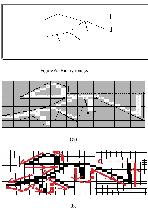
in and popped out of the stack. Figure 5 shows the

[image:9.612.324.566.130.474.2]

original binary image as a sample image. Pixels of

the binary image marked from 1 to

n

are shown in

Figure 6. The flow of search is denoted by a

continuous arrow symbol and jump action is denoted

as dotted arrow.

Figure 6. Binary image.

(a)

(b)

Figure 7. (a) is the labeling components. (b) Pixels of the binary image marked ( ___ ) and the flow of search or jump action marked ( ……).

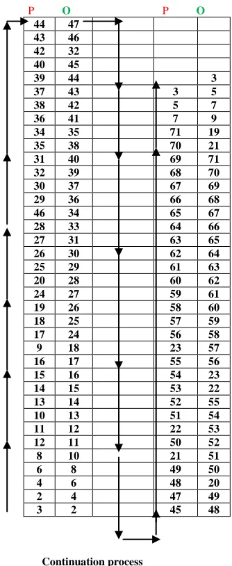
Figure 8, shows the flow of operation row by row

from left to right and dead-end pixels is also shown

by the underline indicator for the entry. It shows the

status of the stack, step by step after each push or pop

operation.

For

the

general

purpose

for

implementation, one can save the color of each pixel

to be added to contents of each entry of the stack as:

(10)

International Journal of Emerging Technology and Advanced Engineering

344 P3 P2 O2P4 O4 P6O6 P8 O8P12 P11 P10O10 O11 O12 P13 O13 P14 O14

P15 O15 P16 O16 P9 P17 O17 P18 O18 P19 P24 O24 P20 P25 O25 P26O26

P27O27P28O28P46P29O29P30O30P32P31O31P33O33 P41P35P34O34P36O36

P38P37O37P39O39P40O40O38O35O41P42O42P43O43 P44O44P45O45O32

O46P47O47P48O48P49O49O20P21P50O50P22P51O51 P52O52P53O53P54

O54P55O55O22P23O23P56O56P57O57P58O58P59O59 P60O60P61O61P62

O62P63O63P64O64P65O65P66O66P67O67P68O68P69

O69P70O70P71O71O21O19O9P7O7P5O5P3O3O3 Figure 8. Flow of operations row by row from left to right.

P : PUSH ; O : POP . Numbers underlined represent dead-end Pixels

The sequence of status structure of the stack, step by

step after each push or pop operation, as in Figure 9.

P O P O

44 47

43 46

42 32

40 45

39 44 3

37 43 3 5

38 42 5 7

36 41 7 9

34 35 71 19

35 38 70 21

31 40 69 71

32 39 68 70

30 37 67 69

29 36 66 68

46 34 65 67

28 33 64 66

27 31 63 65

26 30 62 64

25 29 61 63

20 28 60 62

24 27 59 61

19 26 58 60

18 25 57 59

17 24 56 58

9 18 23 57

16 17 55 56

15 16 54 23

14 15 53 22

13 14 52 55

10 13 51 54

11 12 22 53

12 11 50 52

8 10 21 51

6 8 49 50

4 6 48 20

2 4 47 49

3 2 45 48

[image:10.612.316.483.169.576.2]

Continuation process

(11)

International Journal of Emerging Technology and Advanced Engineering

345 VIII. SAMPLERESULTS

(Old Algorithm) (New Algorithm)

Figure 10. Comparison between the proposed algorithm and Murray Polygon Algorithms. (Right hand side is the new technique and Left hand side is the old Technique). This comparison with Murray polygon is for its the simplicity of implementation and better describing the proposed algorithm.

0 50 100 150 200 250 300

[image:11.612.50.299.164.416.2]

5 10 15 20 25 30 35

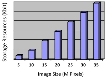
Figure 11. Relation between storage resources (Kbit) and image Size (M Pixels) using the new Technique.

IX. RESULTSANDCONCLUSIONS

Despite a large research literature in image

processing, the labeling connected components are

still difficult and complicated. We tried in this paper

to address new technique for this purpose. Compared

results of well known technique such as "Murray

polygons" and our new novel technique for labeling

connected components of a binary image, which has

many real life applications and particularly, in

medical images, shows that the new algorithm is a

novel one and it is accurate. Results of both

techniques are presented and implemented and tested

on various sample images for comparison purposes.

Such selection of other known algorithm is used only

for easy implementation, and consequently for better

representation our algorithm. All other algorithms in

the literature give good results and one can apply it,

but the one we present is simple, straightforward and

uses minimum storage.

Through this consideration, it has been shown that our

algorithm has at most one scan to be pushed or

popped operation, which is required for each one

complete labeling, as show in the algorithm. This

shown the novel of our algorithm against of other

known algorithms derived by others, such as [1, 5, 7,

18,10, 15] which show that the minimum of scanning

is at least two to four scans in some cases. The

algorithm is applied by scanning the pixels of the

image row by row from left to right, and the same by

applying scanning column by column, from top to

bottom, and the result was approximately the same.

Using the convergence criterion of the sub-images

denoted by I[K,J] at iterations n,n+1, as:

ǀI[K,J]

n+1

-

I[K,J]

n

ǀ

2_{≤ Ɛ, (Ɛ = 10}-3₎

Or using the space

l

p=2

norm of the array

X

[ ]

_lp=2

,

defined as:

for

p

≥ 1 be a real number:

Sto

ra

ge

Re

so

u

rce

s

(K

b

it

)

[image:11.612.79.256.526.659.2]

(12)

International Journal of Emerging Technology and Advanced Engineering

346

ǀǀXǀǀ

_lp₌₂

= ∑(

_│

I[Arr[2i],Arr[2i+1]]

_│2₎p=1/2

,

p ≥ 1

and applying the above formula with a convergence

criteria as: ǀǀ Arr ǀǀ

2

≤

Ɛ, (Ɛ = 10

-3

)

for the

array Arr as:

ǀǀ Arr ǀǀ

2

=

∑ (

_ǀ

I[Arr[2i],Arr[2i+1]]

_ǀ2 ₎1/2

,

0 ≤ n≤ Stackcount

i=0,..,n

approximately, similar results were obtained

for both

cases.

The result obtained due to applying first rows then

columns at each scan, has much significant effect for

accuracy of the results. In contrary, has disadvantage

in term of CPU computer time and storage as well.

The sample results are shown in Figure 10. The

different results show the accurate identification,

allocation and detection of boundary pixels in an

efficient manner. The proposed technique will be

tested more on complicated images, and will be

compared with actual readings of more than two

independent radiologists, to check its accuracy on real

and actual complicated cases for medical images.

Results obtained show that the proposed algorithm is

comparable with other algorithms and cost effective.

The samples in Figure 9 show the comparison

between two known algorithms for labeling connected

components, and its output will be much better than

any available techniques. Such technique is claimed

by the author to be a novel one in term of accuracy,

storage and simplicity with minimum memory

storage. The proposed algorithm can be extended to

be applied for 3-D and higher dimensional images

with more number of gray-scale or colors and will be

generalized for complicated cases and real

applications as that in actual medical images in the

future.

However, since deriving the theoretical upper bound

of the number of scans required to complete the

labeling of arbitrary connected components is of

difficulty, by both our algorithm and others [1, 2, 4, 6,

7, 13, 22, 23], we found also, that the simulation in

the experimental previous example is enough to

describe such new algorithm.

The relation between the image size and required

resource is presented in Figure 11. It shows that the

size of image is basically linear with the memory

requirement and when the number of pixels increases,

the growth of memory requirement becomes slow.

Results obtained by the proposed technique are very

accurate, especially when detecting the boundary

pixels, and compared with the results obtained when

applying the other techniques.

X. SUMMARYANDFUTUREWORK

Main ideas arises from this project tells that the

connected components labelling operator applied by

most of researchers, scans the image by moving

along a row until it comes to a point

p

(where

p

(13)

International Journal of Emerging Technology and Advanced Engineering

347

In this research, we have presented an algorithm for

connected component labeling algorithms based on

the strategy of walk around black pixels to identify

their boundaries. Minimizing the work required for

scanning phase, and the reduction of the time needed

for manipulating the classes for labels are the main

strategies of the proposed algorithm. It shows that the

new proposed algorithm named WAKED AROUND

significantly performs excellent output and much

straightforward to implement compared by the other

available algorithms and produces consecutive labels,

which are convenient for applications. More work

recommended to be done in future for a better

understanding of best labeling strategy based on

scanning rows and columns and after each iteration or

by performing iteration after finishing the whole

labeling depending on the actual colors and not the

black – white binary image. One can think of

removing the similar boundary pixels completely with

similar label, or by approximation of the color pixels

with the average of the 4-Np or 8-Np pixels and

repeating the same process only on the remaining

ones until no more pixels labels exist in the stack. It is

expected that such strategy be much represented and

with minimum CPU computer time for the array used

for labeling , high accuracy and minimum storage,

specially for large images.

ACKNOWLEDGMENTS

This work was supported by the Princess Sumaya

University for Technology, during my sabbatical

leave from King Hussain School for

Computing-Computer Science Department during the academic

year 2013-2014.

References

[1] A. Abramov. T. Kulvicius, F. WÄorgÄotter, B. Dellen. Real-time image segmentation on a GPU. In Lecture Notes in Comuputer Science 6310, Keller R, Kramer D, Weiss J P (eds.), Springer-Verlag, 2011, pp.131-142.

[2] A. Rosenfeld, A. Kak. Digital Picture Processing (2nd edition), Vol. 2. San Diego, USA: Academic Press, 1982.

[3] A. Rosenfeld, J. Pfalts. Sequential operations in digital picture processing. Journal of ACM, 1996, 13(4): 471-494.

[4] A. Tetsuo, N. Asahidai, T. Hiroshi In-place Algorithm for Connected Components Labeling, Journal of Pattern Recognition Research 1 (2010) 10-22 July 1, 2010.

[5] C. Ronsen , P. Denjiver. Connected Components in Binary Images: The Detection Problem. New York, USA: John Wi-ley & Sons. Inc., 1984.

[6] F. Chang, C. Chen, C. Lu. A linear-time component-labeling algorithm using contour tracing technique. Computer Vision and Image Understanding, 2004, 93(2): 206-220.

[7] F. G. Mohammad. International Journal of Scientific & Engineering Research, Volume 4, Issue 5, May-2013 463 ISSN 2229-5518 An efficient multiple pass pixel connectivity labeling method for object detection.

[8] H. Li-Feng, Senior Member, IEEE, C. Yu-Yan , and S. Kenji Suzuki4, Senior Member, IEEE, An Algorithm for Connected-Component Labeling, Hole Labeling and Euler Number Computing, 28(3): 468{478 May 2013. DOI 10.1007/s 11390-013-1348-y.

[9] H. Yah, Labeling Connected Components of a Binary Image, Proceeding of 7'th ICCTA 2007, 1-3 September 2007, Alexandria, Egypt.

[10 J. Hecquard, R. Acharya, Connected component labeling with linear tree, Pattern Recog. 24 (6) (1991) 515–531.

[11] J. Cole, A note on Peano polygons and gray codes. International Journal of Computer Mathematics, 18, (1985).

[12] K. Suzuki, L. Horiba, N. Sugie. Linear-time connected- component labeling based on sequential local operations. Computer Vision and Image Understanding, 2003, 89(1): 1-23.

[13] K. Wu , E. Otoo, K.Suzuki. Optimizing two-pass connected- component labeling algorithms. Pattern Analysis & Applica- tions, 2009, 12(2): 117-135.

[14] L. He, Y. Chao Y, K. Suzuki, K. Wu . Fast connected-component labeling. Pattern Recognition, 2009, 42(9): 1977-1987.

[15] L. He, Y. Chao, Suzuki K. An efficient first-scan method for label-equivalence-based labeling algorithms. Pattern Recog- nition Letters, 2010, 31(1): 28-35.

[16] P. Bhattacharya, Connected component labeling for binary images on a reconfigurable mesh architectures, J. Syst. Architect. 42 (4) (1996) 309–313.

[17] R. Lumia, L. Shapiro, O. Zungia. A new connected components algorithm for virtual memory computers. Comput. Vision, Graphics and Image Processing, 1983, 22(2): 287-300.

[18] T. Assano T. ,T.Hiroshi. In-place Algorithm for Connected Components Labeling, Journal of Pattern Recognition Research 1 (2010) 10-22.

(14)

International Journal of Emerging Technology and Advanced Engineering

348 [20] T. Hattori, A high-speed pipeline processor for regional labeling

based on a new algorithm, in: Proc. Int. Conf. Pattern Recognition (NJ), 1990, pp. 494–496.

[21] W. Kesheng, Otoo E. and Suzuki K. Kesheng Wu, Ekow Otoo and Kenji Suzuki. Two Strategies to Speed up Connected Component Labeling Algorithms. LBNL Tech Report LBNL-59102. 2005.

[22] Y. Ito, K. Nakano. Optimized component labeling algorithm for using in medium sized FPGAs. In Proc. the 9th Int. Conf. Parallel and Distributed Computing, Applications and Technologies, Dec. 2008, pp.171-176.

[23] Q. Hu, G. Qian, W. Nowinski . Fast connected-component labeling in three-dimensional binary images based on iterative recursion. Computer Vision and Image Understanding, 2005, 99(3): 414-434.

About The Author: