Design of Feedback Controller of a Power Plant and Its Stability Study

(1)

International Journal of Emerging Technology and Advanced Engineering

Website: www.ijetae.com (ISSN 2250-2459,ISO 9001:2008 Certified Journal, Volume 4, Issue 2, February 2014)

394

Design of Feedback Controller of a Power Plant and Its

Stability Study

Chandra Mohan Khan

1

, Sukumar Chandra Konar

2

, Chandan Kumar Chanda

3

1

Global Institute of Management and Technology, E. E. Dept. Krishnagar, Nadia-741102, W.B., India

2,3_{Department of Electrical Engineering, Bengal Engineering and Science University, Shibpur, Howrah-711103, W.B., India}

Abstract - This paper includes the theory and practical application involved for determining the stability of power plant including design of feedback controller. The controller aims to stabilize the power system by inter area oscillations and by improving stability from any perturbations. The stability study has been done by using Kharitonov’s four polynomials. The example has been taken with numerical data of the transfer function of 180MW power plant [1]. The result shows that the designed controllers improve the stability of the system and predict the limits of stability. The stability of the system can be incorporated by using Karitonov’s four polynomials and also compared with the help of root locus, Bode plot and Nyquist diagrams.

Keyword – Transfer function of Power Plant, Computer Programming, MATLAB Simulation Result, Stability Analysis by Kharitonov’s four Polynomials, Stability analysis by Root Locus, Bode- diagram and Nyquiest diagram.

I. INTRODUCTION

Concentration on the problem of establishing a normal operating state and optimum scheduling of generation for a power system is important. Block diagrams of simple model of unit including primary and voltage controller in the control system are presented. The real and reactive powers are controlled separately. The load frequency control (LFC) loop controls the real power and frequency and automatic voltage regulator (AVR) loop regulates the reactive power and voltage magnitude. Modern energy control centers (ECC) are equipped with on-line computers performing all signals processing through the remote acquisition systems known as Supervisory Control and Data Acquisition (SCADA) systems [10].

In an interconnected systems load frequency control (LFC) and automatic voltage regulator (AVR) equipment are installed for each generator. Small changes in real power are mainly dependent on changes in rotor angle δ and thus the frequency. The reactive power is mainly dependent on the voltage magnitude i.e., on the generator excitation. The time constant of the excitation system is much smaller than the prime mover time constant and its transient decay much faster and does not affect the LFC.

So the cross-coupling between the LFC loop and the AVR loop is negligible, and the excitation voltage controls are dealt in separately. Hence designing the controller, and then determining its stability range has been presented.The numerical data of modeling and control of a 180 MW power system has been taken as example [1].

II. DESIGN OF AFEEDBACK CONTROLLER

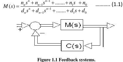
Feedback stabilizability of a linear system with a controller of fixed order has been designed. For SISO systems, let the given nth-order plant [7].

1 1 1 0

1

[image:1.612.330.541.372.478.2]

1 1 0

... ( )

...

n n

n s n s n s n

M s

d s d s d s d

 

   



    ……….. (1.1)

Figure 1.1 Feedback systems.

And C(s) denote the proposed tth-order feedback controller, transfer function of which is as

1

1 1 0

1

1 1 0

... ( )

...

t t

s s s

C s

s s s



 



 

 

   



    ……..(1.2)

And

₁ 1 ₁ ₀

( )

s

_{n t}_

s

n t _{n t}_{ }

s

n t 

...

s

  





 

……….(1.3)

The characteristic polynomial of the resulting closed-loop system.Fig.1.1, shows the feedback system with feedback controller C(s).

Let,

  

:

(

_{n t}_



_{n t}_{ }₁

...

 

₁ ₀

)

T ….(1.4)

Characteristic vector in the form

M x

t

 

……….(1.5)

(2)

International Journal of Emerging Technology and Advanced Engineering

395

The closed-loop characteristic vector ∂ is determined by

1 1 1 1 1 1 0 0 0 1 0 0 0 0

( 1) 2( 1)

0 0

t

t n t

n n

t n t

n n n n

n n

t

x

M n t t

d n

d d n n

d n d n d n





                        _                _                           _                

From Gordan‟s theorem of alternative, it can be shown that, if there exists a nth-order stabilizing controller then there exit x so that

Mtx ˃ 0 ……… (1.6)

For each given matrix A, we have the following. Either

Ax>0, has a solution x ATy=0, y≥0 has a solution y.

But never both, here y ≥ 0 denotes that at least one component of y is positive and no component is negative.

This can also be formulated as a linear- programming problem [9] as follows

min

₍

₎

n nj

j

f x





x

…...……(1.7)

subject to:

( )

n ij nj j

M x 



, i=1,2,……

x

_nj



0

, j=1,2,………

Where Mn(i,j) denote the (i,j)th element of Mn , therefore from (1) ( ) n n t t M x y M M z



     _ _     ………1.8)

From the solution xn of the problem ,a solution x satisfying the inequality condition(1) is obtained with x = y-z, is



a slack variable introduced to avoid strict inequality.

III. EXAMPLE

The example has been taken from with numerical data for modeling and control 180 MW power plant [1]. The given transfer function of the voltage controller is

3 2

6 5 4 3 2

3.15 1.625 ( )

22.9 227.8 2009.3 6300.5 11600.0 4462.5

s s s

M s

s s s s s s

 



     

For a zeroth -order controller, we have

0 1.0 0 22.9 0 227.8 0 2009.3 1 6300.5 3.14 11600.0 1.625 4462.5 0 M                       

For first-order controller, we have

1

1.0 0 0 0

22.9 1.0 0 0

227.8 22.9 0 0

2009.3 227.8 1.0 0

6300.5 2009.3 3.15 1.0

11600.0 6300.5 1.625 3.15

4462.5 11600.0 0 1.625

0 4462.5 0 0

M                           

For 2nd-order controller, we have

2

1.0 0 0 0 0 0

22.9 1.0 0 0 0 0

227.8 22.9 1.0 0 0 0

2009.3 227.8 22.9 1.0 0 0

6300.5 2009.3 227.8 3.15 1.0 0

11600.0 6300.5 2009.3 1.625 3.15 1.0

4462.5 11600.0 6300.5 0 1.625 3.15

0 4462.5 11600.0 0 0 1.625

0 0 4462.5 0 0 0

(3)

International Journal of Emerging Technology and Advanced Engineering

396

A linear programming solution

1 2 3 4 5 6 7 8 9 10 11 12 0.010 0.400 4.000 0.100 0.200 2.000 0.007 0.300 3.000 0.093 0.030 1.000 x x x x x x x x x x x x            

So from the previous formulation x = y-z, we get x as 0.003 0.100 1.000 0.007 0.170 1.000 x                   

Therefore, the transfer function of the stabilizing controller is

2

0.007 0.170 1.000 ( )

0.003 0.100 1.000

s s C s s s     

IV. CHECKING THE STABILITY

The set of monic nth –degree characteristic polynomial after using the controller is of the form

1

1 0

( ) n n n ...

f s s a s   a ……(1.9) For all

a a

_0, ₁

...

a

_n_₁ such that

a

_k



a

_k



a

_k where

k=0,1,…………..,n-1

Then we define the four polynomials

(where

a

_n



a

n



1

) as follows:

3 5 1 1 1

3

1 5

1

1,

( ) ... .min( , ).

n

k k k k

k k k odd

h s a s a s a s j j a j a s 



    



………(1.10)

1

3 5 1 1 1

3 5 2

1,

( )

...

.max(

,

).

n

k k k k

k k k odd

h s

a s a s

a s

j



j a j a s

 









………..(1.11)

( )

i i

a

 

a



x

and

a

i

 

a

_i



( )

x

where i=0,1……,n

Finally, we define the Kharitonov‟s polynomials

11( ) 1( ) 1( )

k s g s h s ……….(1.12)

12( ) 1( ) 2( )

k s g s h s ……….(1.13)

21( ) 2( ) 1( )

k s g s h s .……….(1.14)

22( ) 2( ) 2( )

k s g s h s ………(1.15)

If the four Kharitonov polynomials [12] are Hurwitz then the characteristic polynomial is Hurwitz, i.e. the system is stable in the given region.

Kharitonov's theorem [14],[15] is a result used in control theory to assess the stability of a dynamical system when the physical parameters of the system are not known precisely. When the coefficients of the characteristic polynomial are known, the Routh-Hurwitz stability criterion can be used to check if the system is stable (i.e. if all roots have negative real parts). Kharitonov's theorem can be used in the case where the coefficients are only known to be within specified ranges. It provides a test of stability for a so-called interval polynomial, while Routh-Hurwitz is concerned with an ordinary polynomial.

V. STATE-SPACE MODEL AND STEP RESPONSE ANALYSIS

Let us consider the general nth-order transfer function

1

1 2 1

...

( )

...

n n n n n n n

b

s

b s

b

G s

s

a s

a

  







The „‟state” of a system refers to the past, present and future of the system. It represents all the information that one cares to know about the behavior of the system. The sate variables of a linear system may be defined as a minimal set of variables, x1(t),x2(t),………..,xn(t). Here c(t) is the output and r(t)is the input. By trial and error, the state variables are defined as follows:

(t)=c(t)-h0r(t)

1(t) =x2(t)-h1r (t) 2(t) =x3(t)-h2r(t)

n-1(t)=xn(t)-hn-1r(t)

(4)

International Journal of Emerging Technology and Advanced Engineering

397

Where h0, h1, h2,………..,hn are determined from

0 n 1

h b

1 n n 0

h b a h

2 n 1 n 1 0 n 1

h b a h a h

3 n 2 n 2 0 n 1 1 0 2

h b_ a _ h a _h a h

1 1 0 2 1 3 2 ... 1 2 1

n n n n n

h b a h a h a h  a_h_ a h_ The different state variables are then computed using Runga-Kutta (5th order) method with initial condition and step input.

VI. EXAMPLE

The example has been taken from with numerical data for modeling and control 180 MW power plant [1]. The given transfer function of the voltage controller is

3 2

6 5 4 3 2

3.15 1.625 ( )

22.9 227.8 2009.3 6300.5 11600.0 4462.5

s s s

M s

s s s s s s

 



     

Therefore, the transfer function of the stabilizing controller is

2

0.007 0.170 1.000 ( )

0.0025 0.100 1.000

s s

C s

s s

 



 

To find the stability hyper sphere radius and stability margin of the systems, by the MATLAB statements. We get the large radius of stability hyper sphere ρ(p0)is 0.0076 and stability margin µ(x) is 0.0053.With this controller, the closed loop transfer function of system becomes

( )

1 ( ) ( )

M s G s

C s M s

 

Transfer function:

5 4 3 2

8 7 6 5 4 3 2

0.0025 0.1079 1.319 3.313 1.625 0.0025 0.1573 3.86 50.71 444.7

( )

2670 7475 1205 4463

s s s s s

s s s s s s s

G s

s

   

       



The characteristic equation of the system is

1C s M s( ) ( )0

0.0025s8+0.1687s7+3.9734s6+51.7149s5+447.8236s4+26 75.6969s3+7477.3151s2+12046.875s+4462.5=0

Or,

s8+56.233s7+1324.4667s6+17238.3s5+149274.533s4+ 891898.9667s3+2492438.367s2+4015625s+1487500=0

VII. STABILITY STUDY OF ASYSTEM BY USING

KHARITONOV‟S FOUR PPOLYNOMIALS

Case 1: Disturbance 1% (Due to change of parameters)

If load disturbance of 1% is applied to the system then the Kharitonov‟s four polynomials [12] are become

K11(s),K12(s),K21(s)and K22(s).

K11(s) = 0.99s8+55.670967s7+1337.711367s6+ 7410.683s5+47781.7847s4+882979.911s3+ 2517423.9597s2+4052414.617s+1472625 K12(s) = 1.01s8+55.670967s7+1311.222033s6+

17410.683s5+150767.2753s4+882979.911s3+ 2467573.9803s2+4052414.617s + 1502375 K21(s)=0.99s8+56.795633s

7

+1337.71136s6+17065.917s5 +147781.7847s4+900817.889s3+2517423.9597s2

+3972168.783s+1472625

K22(s) = 1.01s8+56.795633s7+1311.222033s6+ 17065.917s5+150767.2753s4+900817.889s3+ 2467573.9803s2+ 3972168.783s+1502375

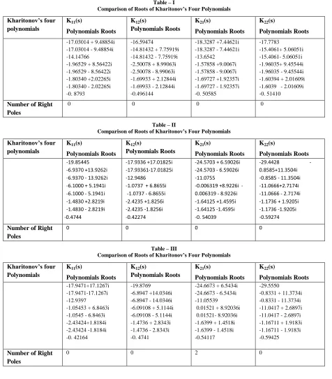
The roots of Kharitonov‟s four polynomials [12] K11(s), K12(s), K21(s) and K22(s) are determined and showed Table – I in APPENDIX. It has been shown that all roots are on the left half of S-Plane so the system is stable.

Case 2: Disturbance 6.5% (Due to change of parameters)

If load disturbance of 6.5% is applied to the system then the Kharitonov‟s four polynomials are become

K11(s),K12(s),K21(s)and K22(s).

K11(s) = 0.935s8+ 52.5781355s7+1410.5570355s6 +18358.7895s5+139571.68555s4+ 833925.4715s3 +2654511.40305s2+4273090.6605s+1390812.5 K12(s)=1.065s8+52.5781355s7+1238.3763645s6+

8358.7895s5+158977.37445s4+833925.4715s3+ 2330486.53695s2+4273090.6605 s+1584187.5 K21(s) = 0.935s8+59.8884645s7+1410.5570355s6+

16117.8105s5+139571.68555s4+949872.3285s3+

2654511.40305s2+3751492.7395s +1390812.5 K22(s)=1.065s8+59.8884645s7+1238.3763645s6+

16117.8105s5+158977.37445s4+949872.3285s3+ 2330486.53695s2+3751492.7395s+1584187.5

(5)

International Journal of Emerging Technology and Advanced Engineering

398 Case3: Disturbance 6.6% (Due to change of parameters)

Load disturbance of 6.6% is applied to the system then the Kharitonov‟s four polynomials are become K11(s),

K12(s), K21(s) and K22(s).

K11(s) = 0.934s8+52.5219022s7+1411.8815022s6+ 18376.0278s5+139422.41102s4+ 833033.5726s3 + 2657003.90202s2+4277102.9522s+1389325 K12(s) =1.066s8+52.5219022s7+1237.0518978s6+

18376.0278s5+159126.64898s4+833033.5726s3+ 2327994.03798s2+4277102.9522s+1585675 K21(s) =0.934s8+59.9446978s7+411.8815022s6+

16100.5722s5+139422 If.41102s4+950764.2274s3+ 2657003.90202s2+3747480.4478s+1389325 K22(s) = 1.066s8+59.9446978s7+1237.0518978s6+

16100.5722s5+159126.64898s4+950764.2274s3+ 2327994.03798s2+3747480.4478s+1585675

The roots of Kharitonov‟s four polynomials K11(s), K12(s), K21(s) and K22(s) are determined and showed in Table – III in APENDIX. It has been shown that two roots of K21 of Khoritonov‟s polynomials are on the right half of S-Plane so the system is unstable.

Therefore the system is stable with load disturbance of 1% to 6.5%.

VIII. STABILITY STUDY OF ASYSTEM BY USING TIME

AND FREQUENCY RESPONSE

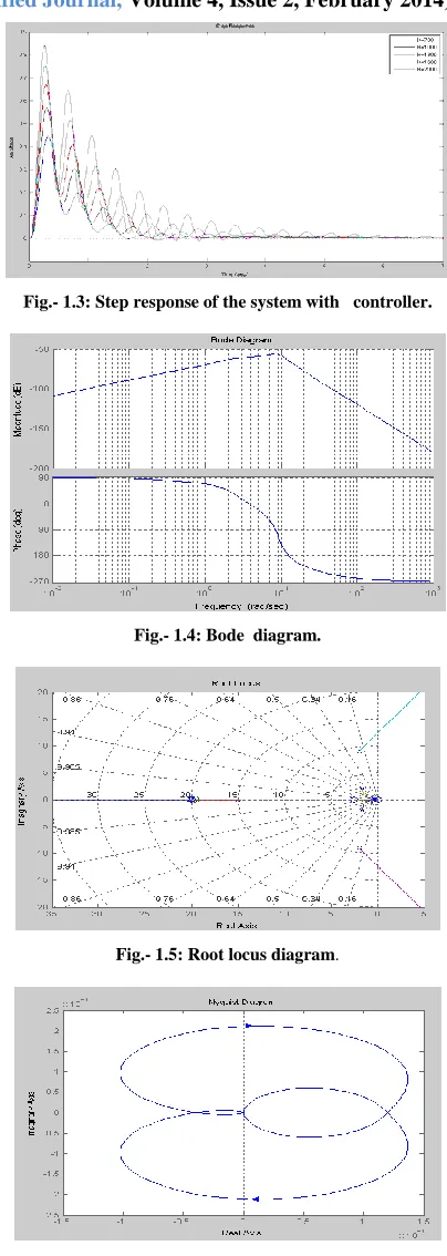
[image:5.612.341.543.125.692.2]

The step response is obtained of the system with and without controller are shown in Figure 1.2 and 1.3 with gain K = 1. Root locus, Bode diagram and Nyqueist diagram are shown in figure1.4, 1.5 and 1.6., Respectively of systems.

Fig. - 1.2: Step response of the system without controller.

Fig.- 1.3: Step response of the system with controller.

Fig.- 1.4: Bode diagram.

Fig.- 1.5: Root locus diagram.

[image:5.612.68.268.518.641.2]

(6)

International Journal of Emerging Technology and Advanced Engineering

399

The Root-locus, Bode diagram and Nyquist diagram of system with gain (K=1) are shown in Figure 1.4 1.5 and 1.6 respectively. In Nyquist diagram (Fig. 1.6), It is shown that the curve crosses the real axis at point - 0.37.

First, if Nyquist plot crosses the real axis at nonzero finite at frequency ω0, then it also crosses the same point where, ω = - ω0 . Moreover, the sign of the crossing is the same at both positive and negative frequencies. This accounts at the point - 0.37. In contrast, if the Nyquist plot crosses the real axis at zero or infinite frequency, then there is just one crossing. Second, when ω = ± ∝ or ω = 0, the curve is not smooth. The cusp phenomena at ω = 0 or ω =

∝ can be overcome easily by rounding to the curve, at the origin so that it is indeed smooth. It is clear that the crossing of the real axis at the origin is a positive one, so range of stabilizing feed gains using can be find out.

The roots of the system at gain (K=1) are as below.

Roots: -20.2839 -19.7149 -15.0016 -2.0001 + 9.0048i -2.0001 - 9.0048i -1.6997 + 2.0262i -1.6997 - 2.0262i -0.5000

It is seen that with gain (K=1), real part of all roots are negative so the system is stable.

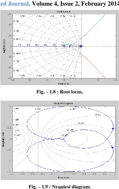
[image:6.612.347.540.119.424.2]

In case 2, when gain is K=1400. The response of the system are given by Bode diagram (Fig.- 1.7), Root locus (Fig.- 1.8) and Nyquiest diagram (Fig.- 1.9)

Fig.- 1.7 : Bode diagram.

Fig. – 1.8 : Root locus.

Fig. – 1.9 : Nyquiest diagram. The roots of the system at gain K=1400 are

Roots: -29.8527 -1.2010 + 14.0594i -1.2010 - 14.0594i -13.5739 + 0.6504i -13.5739 - 0.6504i -1.5161 + 1.0937i -1.5161 - 1.0937i -0.4653

It is seen that with gain K=1400, real part of all roots are negative so the system is stable.

Fig.1.7, Fig.1.8, and Fig.1.9 shows the Bode plot, Root-locus and Nyquist diagram respectively for the magnitude of the gain (K = 1400). The Bode diagram, Root locus and Nyquiest diagram of magnitude of gain (K=2852) are near about same as the magnitude of gain (K=1400). So, the magnitude of the gain (K) lies between the range 1 to 2853 but the curve does not cross the point (-1+ j0).

[image:6.612.72.265.491.612.2]

(7)

International Journal of Emerging Technology and Advanced Engineering

[image:7.612.57.280.132.282.2]

400 Fig. 1.10: The step response of the system. Where K=2853.

The roots of the system at gain K=2853 are given below.

Roots: -33.5890 -0.0002 +17.3487i -0.0002 - 17.3487i -14.0595 -11.8738 -1.4783 + 0.5737i -1.4783 - 0.5737i -0.4206

It is seen that with gain K=2853, real part of all roots are negative so the system is stable.

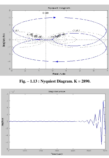
[image:7.612.335.556.136.284.2]

Case 4: We consider the gain of the systems (K) is 2890. The system responses are given by Bode plot, Root locus and Nyquiest diagram.

Fig. – 1.11: Bode Diagram. K = 2890

[image:7.612.335.551.300.611.2]

Fig. – 1.12 : Root Locus when gain K= 2890.

Fig. – 1.13 : Nyquiest Diagram. K = 2890.

[image:7.612.60.275.472.605.2]

(8)

International Journal of Emerging Technology and Advanced Engineering

401

The roots of the system at gain K=2890 are

Roots: -33.6669 0.0289 +17.4187i 0.0289 -17.4187i -14.0640 -11.8516 -1.4779 + 0.5616i -1.4779 - 0.5616i -0.4194

Figure 1.11 and 1.14 represent the Bode and Nyquist plot for gain (K) =2890 respectively. With K=2900, nyquist curve as in Figure 1.13 crosses the point (-1+ j0) which signifies the unstable state of the system.

It is seen that with gain K=1 to 2853 real part of all roots are negative and gain at K = 2890, real part of two roots are positive, which implies the system is stable between K=1 to 2853 i.e. K < 2853 and the system is unstable at

K ˃ 2853.

IX. CONCLUSION

The AVR system of the mentioned power system was simulated for different amplifier gain and observed that the system response was highly oscillatory in nature having high over shoot and settling time. A system stabilizer-rate feedback was introduced in the system and it was found that the system response had been improved but till then some amount of overshoot was presented in the system response and settling time was not so satisfactory. In the next step we introduced a PID controller in the system and observed that the response was very much satisfactory, containing no overshoot and less settling time.

The case study with and without controllers have been performed for stability concerned. However the magnitudes of overshoots are less compared to that of the other case. It is also observed that the maximum overshoot is increasing with the load changes. For stability concerned the transient behavior of interconnected power system the scheme with PID controller is better performance.

We have investigated the stability of the system using Khaitonov‟s polynomials, and are compared with Bode plot, Root-locus and Nyquist plot for different values of gain (K) and also different perturbation. It is observed that system is within stability limits i.e. the real part of the roots of the characteristic equations were negative.

Considering an example, we have investigated the stability of the AVR system of a 180 MW power-plant with different values of system gain.

It was found that the system was stable for gain of 1 to 2853 but if the gain is more than 2853 the system becomes unstable. Using MATLAB technique we have studied frequency response, Bode plot, Nyquiest diagram for stability purpose.

REFERENCE

[1] J.VAN AMERONGEN, H.W.M BARENDS,P.J.BUYS AND G.HODERD “ Modeling and control of 180 MW Power system” .IEEE Transaction on Automatic control,vol,AC-31 No.9 September 1986.

[2] SOHIEL GANGIFAR, M.RAZAEI, “New method to control

dynamic stability of power system thorough wave variable and signal prediction via internet” vol.AC-31 No.9 September

1986.Bowman, M., Debray, S. K., and Peterson, L. L. 1993.

Reasoning about naming systems. .

[3] O. P. Malik, G. S. Hope, Y. M. Gorski, V. A. Uskakov, and A. L. Rackevich, Experiental studies on adaptive microprocessor stabilizers for synchronous generators, in IFAC Power Syst. Power Plant Control, Beijing, China, 125–130, 1986.

[4] D. Das, M. L. Kothari, D. P. Kothari, J. Nanda, Variable structure control strategy to automatic generation control of interconnected reheat thermal systems, Proc. Inst. Electr. Eng.Control Theory Appl., vol. 138, no. 6, pp. 579–585, 1991.

[5] C. S. Chang, W. Fu, F. Wen, Load frequency controller using genetic algorithm based fuzzy gain scheduling of PI controller, Electr. Mach. Power Syst., vol. 26, pp. 39–52, 1998.

[6] S. C. Tripathy, Improved load–frequency control with capacitive energy storage, Energy Convers.Manage., vol. 38, no. 6, pp. 551– 562, 1997.

[7] P. Kundur, Power System Stability and Control. New York, NY: McGraw-Hill, 1994.

[8] T. K. Nagsarkar and M. S. Sukhija, Power System analysis. New Delhi: Oxf. University Press, 2007.

[9] S.P.Bhattacharya, L.H.Keeland, J.W.Howze “Stabilizability

condition using linear programming” IEEE Trans Automat. Contr.

Vol.AC-33,pp460-463,May 1988.

[10] P. M. Anderson and A. A. Fouad, Power System Control and

Stability. USA: IEEE Press, 2nd Edition, 2003.

[11] R.J.Minnichelli,J.J.Anagnost and C.A.Desoer,”An Elementary Proof of Kharitonov‟s “ Stability Theorem with Extensions, ” IEEE Trans.Automat.Contr., vol.AC-34,No.-9,September 198

[12] B.Ross Barmish ,”A Genealization of Kharitonov‟s Four-Polynomial Concept for Robust Stability Problems with Linearly Dependent Coefficient Perturbation,”IEEE Trans.Automat.Contr.,vol.34,No.2, Feb 1989..

[13] K.S.Yeung and S.S.Wang ,”A simple proof of Kharitonov,s theorem,” IEEE Trans.Automat.Contr., Vol.AC-32,pp-822-823, 1987.

[14] Kle and A.L. Tits,”On Kharitonov‟s theorem without invariant degree assumption,” IEEE Trans, Automat.Contr.,vol. AC-36,pp. 1175-1176,July, 2000.

(9)

International Journal of Emerging Technology and Advanced Engineering

402

[16] M. Yao, R. R Shoults, R. Kelm, AGC logic based on NERC‟s new control performance standard and and disturbance control standard, IEEE Trans. Power system, vol.15, no.2.pp. 852 - 857, 2000. [17] P. M. Anderson and A. A. Fouad, Power System Control and

Stability, USA : IEEE Press, 2nd_Edision.

[18] Radoslaw M. Biernacki, Humor Hwang and

S.P.Bhattacharyya,”Robust Stability with Structred Real Parameter Perturbations,”IEEETrans.Automat.Contr.vol.AC-32, No.6, June 1987

[19] M. Aldeen and H. Trinh, “Load frequency control of interconnected power systems via constrained feedback control scheme, Int. J. comput. Electr. Engineering, vol.20, no. 1, pp. 71 – 88, 1994.

[20] A. Rubaai and V. Udo, an adoptive control scheme for load frequency control of multiarea power system. Part – I : Identification and functional design, Part – II : Implementation of test result by simulation . Electr. Power system Res., vol. 24, no. 3, pp. 183- 197 , 1992.

[21] Anderson, B.D.O. ,and J.B. Moore, Optimal control: Linear Quadratic Methods, Prentic – Hall. Englewood Cliffs. New Jersey, 1990.

[22] Kuo. B.C., Automatic Control System , 8th_{Ed. ,Prentic – Hall ,}

India 2004.

(10)

International Journal of Emerging Technology and Advanced Engineering

[image:10.612.71.547.154.696.2]

403 APENDIX.

Table – I

Comparison of Roots of Kharitonov’s Four Polynomials Kharitonov’s four

polynomials

K11(s)

Polynomials Roots

K12(s)

K21(s)

K22(s)

-17.03014 + 9.48854i -17.03014 - 9.48854i -14.14766 -1.96529 + 8.56422i -1.96529 - 8.56422i -1.80340 +2.02265i -1.80340 - 2.02265i -0. 8793

-16.59474 -14.81432 + 7.75919i -14.81432 - 7.75919i -2.50078 + 8.99063i -2.50078 - 8.99063i -1.69933 + 2.12844i -1.69933 - 2.12844i -0.496144

-18.3287 +7.44621i -18.3287 - 7.44621i -13.6542 -1.57858 +9.0067i -1.57858 - 9.0067i -1.69727 +1.92357i -1.69727 - 1.92357i -0. 50585

-17.7783 -15.4061+ 5.06051i -15.4061- 5.06051i -1.96035+ 9.45544i -1.96035 - 9.45544i -1.60394 + 2.01609i -1.6039 - 2.01609i -0. 51410

Number of Right Poles

[image:10.612.75.538.173.338.2]

0 0 0 0

Table – II

polynomials

K11(s)

K12(s)

K21(s)

K22(s)

-19.85445 -6.9370 +13.9262i -6.9370 - 13.9262i -6.1000 + 5.1941i -6.1000 - 5.1941i -1.4830 +2.8219i -1.4830 - 2.8219i -0. -0.4744

-17.9336 +17.01825i -17.93361-17.01825i -12.9486 -1.0737 + 6.8655i -1.0737 - 6.8655i -2.4235 +1.8256i -2.4235 -1.8256i -0.42274

-24.5703 + 6.59026i -24.5703 - 6.59026i -11.0755 0.006319 +8.9226i -0.006319 - 8.9226i -1.64125 +1.4595i -1.64125 -1.4595i -0. 54039

29.4428 -0.8585+11.3504i -0.8585 - 11.3504i -11.0666+2.7174i -11.0666 - 2.7174i -1.1736 + 1.9205i -1.1736 -1.9205i -0.59274

0 0 0 0

Table – III

Polynomials

K11(s)

K12(s)

K21(s)

K22(s)

-17.9471+17.1267i -17.9471-17.1267i -12.9397 -1.05453 + 6.8463i -1.0545 - 6.8463i -2.43424+1.8184i -2.43424 -1.8184i -0. 42164

-19.8769 -6.8947 +14.0346i -6.8947 - 14.0346i -6.09108 + 5.1144i -6.09108 - 5.1144i -1.4736 + 2.8343i -1.4736 - 2.8343i -0. 4741

-24.6673 + 6.5434i -24.6673 - 6.5434i -11.05539 0.01521 + 8.92036i 0.01521- 8.92036i -1.6399 + 1.4518i -1.6399 - 1.4518i -0.54117

-29.5550 -0.8331 + 11.3734i -0.8331 - 11.3734i -11.0417 + 2.6897i -11.0417 - 2.6897i -1.16711 + 1.9183i -1.16711 - 1.9183i -0.59425