A Probabilistic Method of Characterizing Transit Times for Quantum Particles in Non Stationary States

(1)

A Probabilistic Method of Characterizing Transit Times for

Quantum Particles in Non-Stationary States

Hae-Won Kim1_{, Karl Sohlberg}2*

1_{Department of Chemistry, Penn State Abington, Abington, PA, USA} 2_{Department of Chemistry, Drexel University, Philadelphia, PA, USA}

Email: *_{[email protected]}

Received April 10, 2013; revised May 15, 2013; accepted June 24, 2013

Copyright © 2013 Hae-Won Kim, Karl Sohlberg. This is an open access article distributed under the Creative Commons Attribution License, which permits unrestricted use, distribution, and reproduction in any medium, provided the original work is properly cited.

ABSTRACT

We present a probabilistic approach to characterizing the transit time for a quantum particle to flow between two spatially localized states. The time dependence is investigated by initializing the particle in one spatially localized “orbital” and following the time development of the corresponding non-stationary wavefunction of the time-independent Hamil- tonian as the particle travels to a second orbital. We show how to calculate the probability that the particle, initially localized in one orbital, has reached a second orbital after a given elapsed time. To do so, discrete evaluations of the time-dependence of orbital occupancy, taken using a fixed time increment, are subjected to conditional probability analysis with the additional restriction of minimum flow rate. This approach yields transit-time probabilities that converge as the time increment used is decreased. The method is demonstrated on cases of two-state oscillations and shown to produce physically realistic results.

Keywords: Conditional Probability; Non-Stationary Quantum Particle; Transit Time

1. Introduction

There are numerous situations where one might be inter- ested in how quickly a quantum particle moves from one place to another. For example, electron transit times may influence such properties as binary switching speeds and alternating current conductance in molecular electronic devices. As another example, when a chemical reaction intermediate is tautomeric, the time required for the intermediate, prepared in one tautomer, to evolve into the other tautomer, may govern the overall reaction rate. In many cases this exchange of tautomers is essentially a proton transfer.

Investigating theoretically the time dependence of a quantum system begins with solving the time dependent Schrödinger equation (TDSE). Solving the TDSE yields the time dependent wavefunction 

 

t and the corresponding probability density 

 

t 

 

t 2. Consider the movement of a quantum particle between two spatial regions denoted A and B: From the time dependent probability density one may calculate the probability of the particle being in region A at any given time. One may also calculate the probability of the particle being in

re-gion B at any given time, but the time dependent wavefunction does not directly yield the time it takes for the particle to travel from A to B. In order to attain quantita- tive knowledge of the time-dependence of the flow of a quantum particle, it is essential to develop methods to extract this information from the time-dependent wavefunction 

 

t and/or the corresponding probability density 

 

t . Owing to the non-commutativity of the quantum position and momentum operators, the time required for a quantum particle to get from one spatial location to another must be defined differently from the analogous quantity for a classical particle. Here we present an approach that expresses transit time in terms of probabilistic confidences.

(2)

transfer [3], superexchange today being of central rele- vance in molecular transport junctions [4,5]. Coalson has investigated the accuracy of time-dependent perturbation theory methods to treat nuclear-electronic coupling in long-range electron transfer by benchmarking results for a model Hamiltonian to its exactly solvable limit [6]. Such long-range electron transfer is relevant in a wide variety of donor-bridge-acceptor systems [7]. These studies give insight into the time dependence of electron transfer, but none recover the transit time.

A special case from the class of problems encom- passed by the question, “How fast does a quantum particle move from A to B?” is the question of tunneling time through a potential barrier. Tunneling time has been a matter of considerable discussion almost since the incep- tion of quantum mechanics. Valuable reviews have been presented by Hauge and Støvneng [8] and more recently by Winful [9]. The latter review is especially valuable for its appendix, which addresses conceptual questions about tunneling. One issue of sustained interest, apparent su- perluminal transport across the tunneling barrier, now appears largely resolved [10], as it has been demonstrated that causality is not violated [11,12].

Although we consider a more general problem, the transit of a quantum particle from one spatial location to another, two “tunneling time” papers are more than tan- gentially relevant to the present work: First, Dumont and Marchioro [13] have given a clear explanation why the question, “How much time does a tunneling particle spend under the barrier?” is ill posed. The difficulty with this question is that its answer would require the simul- taneous evaluation of observables corresponding to non-commutative operators. Dumont and Marchioro argue, as we alluded to above, that the question must be posed in a probabilistic manner. Second: Baskin and So- kolovskii [14] addressed tunneling time by generalizing the classical concept of transit time to the quantum mechanical case. We too have found it useful to reference a classical case, but rather than generalizing from a deter- ministic classical system, we draw analogy to a pro- babilistic classical system.

In this paper, we present a new way to characterize transit times by analyzing the time-dependent probability density. We then demonstrate the method on the two different systems that display two state oscillations. The movement of the quantum particle is investigated by following the time development of a localized wavefunction, which is expanded in a basis of eigenfunctions of the time independent Hamiltonian using standard methods. From the time development of the wavefunction, we show how to calculate the probability that the particle, initially localized in one orbital, has reached a second orbital after a given elapsed time; or conversely, how to calculate the time that must elapse for the particle to

reach the second orbital with a given probability. Collec- tively, we refer to these questions as the “electron orbital-occupancy problem”. A related question, “How fast can a quantum state change with time?” (under the con- trol of a time-dependent Hamiltonian) is the subject of a work with that title by Pfeifer [15].

2. Two State Oscillations

The time dependence of two-state oscillations is a topic from introductory quantum mechanics. We discuss such oscillations here principally to define the time-dependent probability function for a specific case to be analyzed here, but also to introduce the notation that will be used in the balance of the paper.

Consider an electron that oscillates between two spatially localized states (These localized states could represent the source and drain of a two-terminal molecular electronic device under no applied potential, or the donor and acceptor in a DBA system, but for purposes of this study we consider two generic spatially localized non- eigenstates). We want to find out how long it takes for an electron that is initially prepared in one such state to reach a second state. Such a non-stationary state might be prepared with shaped laser pulses [16] or a sudden change in potential [17]. Here we will not concern our- selves with how the spatially localized state is prepared, but rather with how to analyze its time-evolution. To begin the problem we first solve the time-dependent Schrödinger equation (TDSE) by expanding the spatial wave function in a linear combination of eigenfunctions of the time-independent Schrodinger equation (TISE) according to canonical procedure.

Consider a time-independent Hamiltonian Hˆ for an electron in which there are two eigenstates i that obey

the relations:

1 1 1 2 2

ˆ _, ˆ

H E H E2. (1)

The TDSE for this system is: ˆ

i   t H . (2)

Given that ˆH is time-independent, if we let:

   

Φ

T t r

  , then the system separates into time dependent and time independent parts with the solution of the time-dependent part being, T t

 

exp



iEt 



. Expanding the spatial wavefunction Φ

 

r in a linear combination of eigenfunctions of ˆH, it follows that the general form of the solution to the TDSE is,

   

Φ k kexp



k



T t r c iE t k

  



  , (3)

where the ck are the expansion coefficients at t0.

Since the basis functions are eigenstates, the probability of finding the system in a particular eigenstate at time is,

t

 

*

k k c

(3)

For our purposes, however, it is more useful to consider an expansion in non-eigenstate functions. For example, suppose that we describe a localized electron in a mole- cule as an expansion in atomic orbitals (AOs). We can follow the flow of charge by observing how the AO expansion coefficients vary as the time-dependent wavefunction evolves in time. Ultimately, we want to address the question; how long does it take for an electron that is initially localized in one AO to reach a second selected AO?

Suppose that the two eigenstates (1 and 2) of the two-state system are expanded in a basis of two AOs;

1

 and 2. In this basis, the TISE in secular form is,

det E Es 0

Es E

 

 

 



  (4)

where  i Hˆ i ,   i Hˆ j , and s  i j

The solutio

. ns are,



 



1 1 ; for which

E    s ₁₁₂ (5a)



 



2 1 ; for which

E    s 2 12 (5b)

If we use the approximation, s_ij, the roots are,

E  . (6) Both eigenvalues are displaced from the site energy  by an amount dependent on the coupling matrix ele- ment . Since  just sets the zero of potential, we can take the eigenenergies to be E .

Suppose that we initially localize r electron by ou placing it exclusively in the AO 1. At t0 the spatial wavefunction, written as an expansion in AOs, is,





1 1

Φ r t, 0  1 0₂. (7)

To write the time-dependent wavefunction, we must express this in the basis of eigenfunctions of ˆH. In oth-er words, we must find the ck in Equation (3). This is a

standard change from an AO basis to a molecular orbital (MO) basis. From the definitions of k in Equations (5a)

and (5b), it follows that c10.5 and c 0.5. We can now write the time dependent wavef2 unction:

   





1





Φ

0.5exp 0.5exp

T t r

i t  i t 2

 

      (8)

To follow the time evolution of the wavefunction in space, we need to transform from the MO basis back to the AO basis. Using the Euler relations, we obtain the time dependent AO-occupancy probabilities as:

 

2





1 cos t

     (9a)

 

2





2 sin t

     (9b) As expected, . Note that the fre-

qu ion between the tw

 

1

 

2 1

    

ency of oscillat o functions is  . Note also that the oscillation frequency depends on e energy difference between the states, the greater the energy difference, the greater the frequency.

In oscillatory systems the period of o

th

scillation

 

 ncy bears a reciprocal relationship to the freque



 2π



where

 

 is the angular frequency. As e example above, a bound quantum system in a non-stationary state is characterized by such a frequency, (or frequencies in a system with more than two levels). The related period(s), however, is(are) a physically unsatisfactory metric of the lifetime of the associ- ated spatially localized state. In Section 5 we demonstrate that this quantum exchange frequency suggests a rapid exchange between tautomers in cases when one would likely have to wait an aeon for one tautomer to evolve into another. The present paper addresses this dilemma.

Solution of the TDSE as outlined in this section yield shown in th

s th

3. Professor Office-Occupancy Problem

ssical e time-dependence of occupancy for each spatially localized orbital (AO). This standard procedure is easily generalized to an arbitrary number of AO basis functions. It is a standard result in quantum mechanics and answers the question, “what is the probability that a selected AO is occupied at a specific time t?” Herein we will demonstrate how to analyze the time dependent probability function to address our central question: Given that the electron is initially localized on one atomic orbital, how much time must elapse for the electron to reach the second orbital with a given probability? In the next section we look at an analogous classical system in order to develop the methods to answer this question. The system we look at is a “professor office-occupancy problem”.

To develop the methodology, we first consider a cla problem analogous to the “electron orbital-occupancy problem”: We ask the question; given a function that describes the probability of a professor being in her office as a function of time, what is the probability that the professor has occupied her office at least once during some elapsed time period? We term this the “professor office-occupancy problem”. Exploration of this classical problem allows us to identify the variables that are important in the electron orbital-occupancy problem and to determine what assumptions might be necessary to produce a physically reasonable answer. Our approach is based on evaluating the time dependent probability density





 

t 2



at a fixed time increment. We find that

(4)

electron orbital-occupancy problem. In addition to studying the time dependence of electron orbital occupancy, the method is also demonstrated for proton exchange in a double well potential.

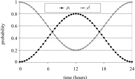
The professor office-occupancy problem is defined as follows: We take the probability of finding a professor in her office, 

 

t , to be a sinusoidal function of time with a period of ours and an amplitude of 0.79; a minimum at midnight at which there is 1% probability of finding her in her office; and a maximum of 80% probability at noon. The function is shown in Figure 1 (In this analysis we assume all days, whether weekend, weekday or holiday, are equivalent. A more complicated function with 7-day or 30-day periodicity could be used, but this would only serve to obfuscate the analysis without introducing any new physics). The probability function may be written as,

 

24 h





0.405

t

  0.395 cos 2 πt 24 , (10) where is time in hours. The area under the curv

of as a two-state oscilla- tio

t the professor’s office an

t e, 9.72

hours/day, is the average amount of time the professor spends in her office each day.

This system can be thought

n. The professor is either “in” her office or “not in” her office, and she oscillates between these two “states” according to the assumed probability function (10). Now let us address the question; given a specific start time, how much time must elapse for the professor to have visited her office at least once with a selected probability? One way of thinking about the question is this: If a student comes to the professor’s office, how long must the student wait to be 90% confident (or 99.999% confident) that the professor will show up?

The student could show up a

d wait. Alternatively, the student could check the office periodically. As the frequency with which the student checks the office approaches infinity, the elapsed time to finding the professor must converge to the period

ρi i

0 0

pr

ob

ab

ilit

y

time (hours)

6 12 18 24

[image:4.595.60.285.555.687.2]

0.2 0.4 0.6 0.8 1

Figure 1. Probability  of finding a professor in her office as a function of time together with the probability  that the office is not occupied.

of time the student would have to wait at the office door.

3.1. Simple Probability Analysis

r office-occupancy

k

Convergence of the time to achieve a given confidence level with increasing sampling frequency is therefore a necessary condition for the validity of any approach that is based on repetitive sampling of the probability function. In the next subsection we show that simple multiplication of the probabilities extracted from the probability function fails in this regard.

We begin our analysis of the professo

problem by studying what happens if the student checks the professor’s office periodically. The naive approach assumes probabilistic independence, in which case the probability that the office has never been found to be occupied in N samplings not

N

P is,

 





1, , 1 not

N k N

P 



_ _  t , (11)

where k

 

t is the probability of the office being occupied in a specific sampling event k. The probability that the professor has been found in her office is then



1 not



N N

P  P . This approach may appear to give rea- s for widely separated sampling events sonable result



  t tk tk10



, but obviously the assumption that

 

t

 and   



t t



nseque

are probabilistically independent wed. C ntly, the method fails as t 0

is fla o   .

This failure can be seen by considering four c ) The student looks for the professor at exactly noon each day. 2) The student looks for the professor at noon and midnight each day. 3) The student looks for the pro- fes-sor at noon and 2 seconds after noon each day. 4) The student looks for the professor at noon and every 2 seconds thereafter until 12:00:08 pm each day.

Applying Equation (11) to the four cas

ases: 1

es described above yields the results in Table 1, which shows the day on which the probability of having found the professor exceeds 99.999%. In case 1, after N consecutive days the probability that the student has ated the professor is 1

 

0.2

loc

N N

P   . This expression converges to 1.0 wit , a physically sensible result. In case 2, after

h increasing N

M consecutive days the probability that the student ha located the professor is s 1



0.198



M. This converges to 1.0, but slightly more if the student checks only at noon, again a physically sensible result. By checking at midnight in addition to noon, the student increases the probability of finding the professor, but only by a little because the professor is very unlikely to be found in her office at midnight.

For case 3, since

rapidly than









(5)

9 % probability, based on looking for her at different times of

probability of finding the professor

Table 1. The day the professor is found in her office with 99.99

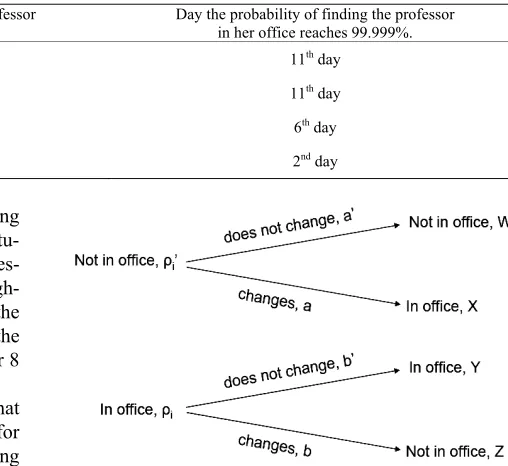
the day under the assumption that these samplings possess probabilistic independence.

Formula to calculate the probability the professor Day the

has been found in her office. in her office reaches 99.999%. Case 1 1 − 0.2N₁₁th_day

Case 2 1 − ( N₁₁

6 day

1 2

0.2 × 0.99) th_day

Case 3 1 − (0.2 × 0.2)N th

Case 4 − (0.2 ×··· 0.2)N nd_day

ompletely unreasonable. The probability is converging

that c

to 1.0 more rapidly than in case 1, only because the student is making two attempts to find the professor at essentially the same time each day! Case 4 further high- lights the failure of this approach. Table 1 shows that the professor is found 10 days earlier simply because the student is looking into the office every two seconds for 8 minutes each day, instead of simply checking once.

The reason for the failure of Equation (11) is

 

t is very strongly correlated to



  t t

_

for

t

 owing to the continuity of the ving probability function

small time evol

 

t

[image:5.595.278.532.111.344.2]

 . In the next section we describe an approach that accounts for the correlation between sampling events to produce a predicted time to achieve a given confidence level that converges with increasing sampling frequency.

Figure 2. Conditional probability tree diagram where: ρi

tim is theprobability that the professor is in her office at e

 i

t = i, p , is the probability that she is not in her office time t = i, and

at

 1

i i

ρ = ρ, at any time ti.

given a 3.2. Conditional Probability

During a discrete time-step

 

t , the condition of the

ram, is the probability that the “s

professor being in the office either change or stay the same. In general, the probability that the condition changes may depend on the initial state. We can represent the evolution during a time-step with a tree as de- picted in Figure 2.

In the tree diag

will

a t

tate” changes given that he professor is not in her office and b is the probability that the state changes giv-en that she is in her office (a  1 a and b  1 b). We can write the probabilities in th at

t t as:

of being e office





1 1

i  X Y i a i b , (12a) 





1 1

i W Z i a b

_     _i . (12b)

If and can be determined froma b _i and i1 (and i and i1) it is then possible to determine the proba ity that professor was never in her office. The probability is given by the probability that the office was not occupied at time



bil the



0

0,

t   times the probability that the state did not cha h subsequent time-step



a  1 a



. In other words, given that the office was not time t i , if the probability that the state did not change between time t i

nge on eac

occupied at

 and time t i 1 is

by i i, 1 , then the probability t at h the office was ever occ is given by,

n upied





0 0, , , 1 1

not

i i i N

P 



  a 0



i0, ,N ai i, 1 . (13)

In fact, Equations (12a) and (12b) are dependen we can therefore only solve for in terms of Whil a

t and e a

m

b.

definitive relationship between a and b is not obvious, both a and b values ust be confined by

 

0 a b, 1 because they repre nt probabilities. By rearranging Equation 12a) and (12b), we obtain the

ressions.

se s (

following exp



i i

 

i – i 1



i

a   b  _  (14a)



i i





i 1– i



i

b   a    .

Using probability function Equation ( tionships of (14a) and (14b), we can fin al

(14b)

10) and the rela- d the range of lowed values of a and b at each time-step.

Consider as a specific example, the set of conditions:

0.6 i

  , _i 0.4, i₁0.7, i 1 0.3. It follows that for this specific set of conditions,

 

4 6 1 6

b a . (15)

We haven’t identified another and , but we do know

relationship between a that



0 a 1



and b



0 b 1



. The range of allowed values of a and for this example case is shown with th line

(6)

segment on

ed values the LHS graph of Figure 3.

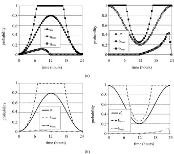
Based on analyzing the allowed ranges for a and b, the minimum and maximum allow of



b0,1



and



a b a0,1



using two samp - steps, (0.5 hour and 0.1 hour) are shown in Figures 4(a)

rom th we see that amin and bmin decrease as the time-step gets smaller. This is a physically sensible result: As the time step decreases, probability that the state changes during the time step also decreases (i.e., the state is very unlikely to change during a very short time interval).

There are many mathematically allowed solutions of Equation (14) for a

ling tim

the

and To obtain the physically m

e

and 4(b). F e figures

b.

eaningful solution, a second condition on a and b is required. One obvious possibility is a b 1. Using this condition, direct application of Equation (1 prod ces the same unphysical result as the sim bability approach. The predicted time to achieve a given confidence level does not converge with decreasing time-step. We conclude that this obvious additional condition on a and b is not the physical one.

3) ro

u ple p

We note that physically, and b represent the probabilities of the “occupied” and “unoccupied” states changing during the given time interval. While we do not know the specific values of and for any given

a

a b

1

≈ρ2≈0 1.0

0.5

0.5 1.0

-0.5

-1.0

a b

1.0

0.5

0.5 1.0 -0.5

-0.5

-1.0

a b

ρ1≈2≈0

ρ1≈ρ2≈0

[image:6.595.313.536.144.293.2]

ρ1≈ρ2≈1

Figure 3. LHS: allowed ranges for and b for the set of conditions:

a 0.6

i

ρ  , _i0.4, ρi+10.7, ρi+10.3. RHS:

extrema of allowed values of a and in general. b

ρi

i



0 0

pr

oba

bi

lit

y

time (hours)

6 12 18 24

0.2 0.4 0.6 0.8 1

0.8

0.6

pr

ob

ab

ilit

y

0.4 amax

bmax

amin _0.2

bmin 0

0

time (hours)

6 12 18 24

1

(a)

ρi

i



0 0

pr

ob

ab

ilit

y

time (hours)

6 12 18 24

0.2 0.4 0.6 0.8 1

amax

amin

bmax

bmin 0

0

pr

ob

ab

ilit

y

6 12 18 24

0.2 0.4 0.6 0.8 1

time (hours)

(b)

Figure 4. (a) Allowed range of and values for conditional probability for professor office-occupancy problem. Also plotted are the

a b

 

ρ t , amin

, with amax, with The plots are made for 0.5 hour time intervals. (b)

Al-s

min min

lowed range of a and b value for conditional probability for professor office-occupancy problem. Also plotted are the

 

ρ t , with amax and

a and ρ

 

t bmax, b .

 



ρ t with bmax . The made for 0.1 hour time intervals. The spacing of data

points is so small that individual points have been replaced with an interpolating curve for visual clarity. Note that amin and

are smaller than in Figure 4(a) where a lar time step was used. , bmin

ger

plots are

min

[image:6.595.127.467.343.644.2]

(7)

ep

time interval, it is physically reasonable that as the time is decreased, the probability of the state changing

st

during any one time step decreases. In the limit of de- creasing time step therefore, a and b should take on their smallest allowed values. We therefore used the slowest mathematically allowed flow of probability by using a b minimum where we denote a a min and

min

b b . The case



a b minimum



represents the fewest office occupancy state changes that produce i

and i1, from i and i1. This is the physically meaningful additional condition on a and b.

In the range



0 t 12



, the probability that the office is occupied is increasing, therefore the minimum change is accomplished by setting b0, which produces a a min. Here, if the office is occupied it remains so, if it is not, there is a small probability of a change in the state



a_min



. Similarly, for



12 t 24



, the probability that the office is occupied is decreasing. The minimum change is accomplished by setting a0, which produces b b min. In this case, if the office is empty it remains so, but if it is occupied there is a small probability of a change in the state



b_min



.

One might argue that the state of the system could change during the first time interval (or any subsequent tim

fig the elapsed time at which we can be 90% confi-

e interval) regardless of how short the time increment is, in which case a1, not its minimum allowed value. This is true, however, we seek to place a confidence on the office occupancy within some elapsed time. While the rapid state change may happen, to specify a confidence that the state change has happened we must base our analysis on the slowest rate of state change that is consistent with the probability function.

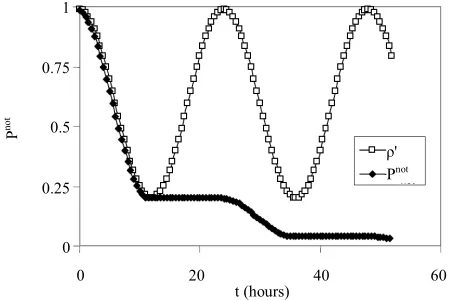
[image:7.595.311.538.335.485.2]

Using the above analysis, we can put rigorous upper and lower bounds on the flow of probability. To obtain the upper limit, we use a a max. In this case the office is occupied the first time we look. To obtain the lower limit we use a a min, which produces Pnot

 

t as shown in

Figure 5. Note that _Pnot_{drops below 0.1 at 30.5 hours.}

(Half-hour time steps were used to generate the ure). This is

dent that the professor has been in her office at least once. The results (collected in Table 2) show that as the time-step gets smaller, the approaches using simple probability, and conditional probability using a b 1, predict that the time to 90% occupancy probability decreases to zero with increasing sampling frequency, a physically nonsensical result. Only the conditional probability analysis with the assumption of minimum flow

produces a result that converges.

3.3. Validation by Monte Carlo Simulation

3.3.1. Simulation Methods

Carlo he time-dependent probabil- To validate our findings, we performed Monte (MC) simulations based on t

ity function (10) for both the simple probability and conditional probability approaches. We compared the results to direct application of equations (11—simple probability

0 0

t (hours) 20

P

not

40 60

0.25 0.5 0.75 1

ρ' Pnot

Figure 5. Time dependence of ρ not

(the probability that the office is not occupied) and P

r (the probabilistic conf

0% like a

i-dence that the office has neve been occupied between

= 0

[image:7.595.57.538.608.730.2]

t and t) based on conditional probability analysis. ly to h ve been in her office at least once

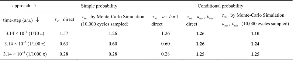
Table 2. The elapsed time (hours) at which the professor is 9

 

90 . The

b p

oldface result is the physically meaningful one. The other results are based on the flawed assumption that samplings of the ct denot robability function are independent events. Monte-Carlo denotes the result of a Monte-Carlo simulation. Dire es direct application of the noted equation.

approach Simple probability (Equation (11)) Conditional probability (Equation (13)) direct 90 amin, bmindirect 90 amin, bmin

Monte-Carlo 90 a b 1

time-step (hour)  90 direct 90 Monte-Carlo

60 min (1 hr) 8.00 30.5

6.00 31 30

9.00 8.00 31

30 min (1/2 hr) 6.50 6.00 .7

15 min (1/4 hr) 5.00 4.75 4.75 31 30.8

10 min (1/6 hr) 4.33 4.17 4.17 31 30.9

1 min (1/60 hr) 1.68 1.65 1.68 31.0 30.9

(8)

ana —cond al probabili alysis). For consistency, in all cases we determined the e he r is 90% ly to have b n her office

lysis) and (13 ition ty an

elapsed tim een i

w n the professo like at least once

 

₉₀ .

In the first set of MC simulations, (simple probability) the “1st_{visit time” is found by starting at time}_t_₀_of the first day a d advancing in discrete time steps n t. At each time-step a random number is chosen between 0 and 1. If the random number falls under the probability curve

 

t

 the professor is taken to be in her office and the answer is obtained. If the random number falls on or above the curve, another time-step is taken and so on until we get the 1st_{visit. We look at all first visits and} find the time of day when 90% of the first visits have occurred. We continued to follow the professor’s movement beyond the 1st_{visit to validate whether the simula-} tion procedure reproduces the 

 

t profile. (This allows us to look at the office-occupancy problem without an artificial day-cycle boundary.) One or multiple consecutive in-office-states constitute a single visit. Most of the visits are in the middle of the day-cycle as expected. This approach reproduces the 

 

t profile with the professor spending on average 9.72 hours per day in the office as shown in Figure 6.

For comparison, for direct application of Equation (11), the time the professor is found in her office at least once with 90% probability is determined by setting the value of Equation (11) to 0.1 and solving for t. Here k runs from 0 to N and t  k t. The probability is given by the probability that the professor was not in her office at time t0,

 

₀ times the probability that she was not in her office at the end of each subsequent time-step

 

_i . The product is carried out stepwise, incrementing N by 1

0 0

time (hours)

6 12 18 24

0.2 0.4 0.6 0.8 1

pr

ob

ab

ilit

y

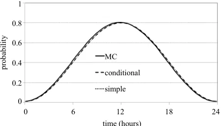
MC

[image:8.595.60.287.497.626.2]

simple conditional

Figure 6. Comparison of ρ

 

t

unt

profiles based on simula-tions with ρ

 

t

n

function of Equa

flow

tion (1): MC = Monte- Carlo simulatio , conditional = simulation with conditional probability with minimum , simple = simulation based on simple multiplication of probabilities. For the Monte- Carlo simulations 10,000 day-cycles were used. All of the simulations reproduce the original ρ

 

t function and pre-dict an average of 9.72 hours spent in office per day.

manner as the simple probability approach described two paragraphs above, but with one difference; at each time- step we compare the random num to the amin in the range 0 t 12

il drops b 0.1.

A M nte Carlo sim lation based condition l probabil- inimum w is obtained in ry similar

ber not

N

P o

elow u flo

a a ve ity with m

  and bmin, for the range 12t 24, instead of comparing the random number to 

 

t as done in the simple probability approach.

Direct application of Equation (13) was accomplished analogously to direct application of Equation (11). This product, and all other simulations described in this ma-nuscript, were carried out using program ATLAB [18].

3.3.2. MC Results

In

M

Simply checking the office with infinite fre- arantee that the professor will arrive

Table 2 we report the results of our calculation using varying time-steps. The results show that the answer given by the simple probability approach depends on how frequently the office is checked and converges to zero as the time step is decreased, a physically nonsensical result.

quency does not gu immediately!

As shown in Table 2, the simulation based on the condition of minimum flow produces an answer that is independent of time-step and is exactly the same as the analytic analysis shown in Figure 5, and the direct application of Equation (13). The minimum flow conditional probability approach also produces the correct

 

t

 profile as shown in Figure 6 with a total office time of 9.72 hours per day-cycle.

In the approach using conditional probability with minimum flow rate, since a a min0 from noon till midnight, no first visits are found during the final 12 hours of a day-cycle. As a result, some days have no visits at all and the answer, time ‘till the first visit, is greater than 24 hours (It is important to note that the professor

can arrive at her office within the first 24 hours, or 12 hours or any shorter time interval, but 90% confidence is not achieved until later). Thi achieves our re- quirement of obtaining a solution to the problem that converges with decreasing time-step.

There is an important feature of quantum mechanics that merits note here: In a quantum system, the time- dependent wavefunction (and its corresponding probability density

s approach

 

t

(9)

collapse the wav ction into a stationary state. It is important to draw a distinction, however, between carry- ing out a measurement of the system and evaluating a probability density function. To analyze the mathemati- cal properties of



efun



t

 we may evaluate it at numerous values of t without altering the function, just as inte- grating the absolute square of a 1D spatial wavefunction

 

2

x

 over the interval



   x



to establish that it is properly normalized does not collapse the system into a single-valued position state, which would be rep- resented by a delta function. For this reason, we may use the analogy to the classical office occupancy case to in- form us of how to analyze the time evolving probability function. In the ensuing sections we apply the minimum flow conditional probability quantum

ical systems.

analysis to two mechan

4. Electron Orbital-Occupancy

We have applied the methods developed above to the orbital-occupancy problem where _

 

_t __sin2



__t _



gives the time dependence of electron occupancy for orbital 2 (See Equation (9b)). The oscillation frequency is  . In our calculations we took the values of  and  to be 1. The cycle length is therefore

dvances by orbital occ

ich the electr

i

π

π).

u-

n is

lit (The function repeats every time t a

The results of our studies for the electron

o pancy problem are collected in Table 3, which shows the elapsed time (fraction of a cycle) at wh

90% likely to have occupied the second orbital at least once. Note that just as in the professor office-occupancy problem, th mple probability approach produces the physically unreasonable prediction that as the sampling rate increases, the time to 90% oc upancy probabi y converges to zero. The simple probability and a b 1

e s

c

 

Monte Carlo simulations produce the same unphysical result because they are based on the same flawed assumption of uncorrelated probabilities. The approach of using conditional probability with minimum flow rate converges to 1.25, indicating that at about 125/314th_{of an} oscillation cycle, the electron has reached the second

“acceptor” orbital with 90% probability.

While the results presented here employ a basis of two atomic orbitals, the extension to a larger basis is straightforward. Numerical integration of the TDSE for a non-stationary state representing an initially localized electron yields a discrete representation of the time dependent state vector. Upon transformation from the basis of eigenstates of the TISE to the AO basis, the squares of the AO expansion coefficients are the time dependent occupancy probabilities. Application of the conditional probability analysis described above to a selected orbital will give the elapsed time to expected occupancy of that orbital.

While our example analyses the time dependent probability function arising from a non-stationary wavefunction evolving under the influence of a time-independent Hamiltonian, it can, in principle, be applied more gener- ally. The time-evolving probability need not be based on a time-independent Hamiltonian. In the case of a time- dependent Hamiltonian, the methods of finding the time-dependent wavefunction would be different, but our method of analyzing the probability function would still apply.

5. Proton Transfer across an Asymmetric

Double Well

As a second application of our conditional probability analysis we consider the exchange of a proton across an asymmetric double-well potential. Here we employ the quantum mechanical model of Hameka and de la Vega [19]. The Hamiltonian is taken to be time-independent and of the form,

0 ˆ

HH H. (16) Here _H0_{describes a symmetric double-well poten-} tial having the lowest two eigenenergies _E0___{, where}  represents half the splitting of these lowest two eigenenergies. The fundamental oscillation frequency is

0 2

   . The perturbation term, H x d

   , intro-

[image:9.595.57.539.637.736.2]

duces the asymmetry to the potential. Here  is the

Table 3. The time (a.u.) at which the electron is 9 y t result is the physically meaningful one. The other results are b ity function are independent events. The oscillation frequency

0% likel o have occupied the second orbital at least once. The boldface ased on the flawed assumption that samplings of the probabil-is β ,where β=1 and 1. The cycle length is .

Conditional probability

π

approach Simple probability

time-step (a.u.)  90 direct 90

 by Monte-Carlo Simulation (10,000 cycles sampled)

90

 a b 1 direct

90

 amin, bmin

direct

90



min

by Monte-Carlo Simulation (10,000 cycles sampled)

min

,

a b

3.14 × 10−1_(1/10_π_{) 1.57} _1.26 _1.26 _{1.26 1.10}

3.14 × 10−2_(1/100_π_{) 0.63} _0.60 _0.60 _{1.26 1.24}

(10)

energ between the of the asymmetric double well, is their spatial sepa a

y difference classical minima

d ration

nd x is the di splacem oo

m eka and de la eg eral

as ter

ent c rdinate. Based on this a [19] define a gen

odel, Ham V

ymmetry parame  2, and show the os- c

  that

illation frequency

 

 as a function of th mmetry param ter is,

e asy e

2 0 1

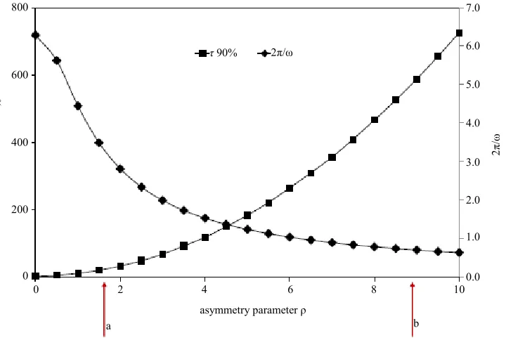
   . (17) A traditional measure of ifetime in quantum systems is,

l

2π

 . By this measure, the lifetime decreases with increasing asymmetry (increasing 1



  ). We have posed the question; given he deeper well A is initially occupied, how g must one wait to be 90% confident that the

that t lon

proton has sampled sh well B? (As before, we denote this period

allower 90

 ). A plot of 90 versus the asymmetry parameter is g

co

iven in Figure 7, where it is mpared to the traditional measure of lifetime

2π

  .

quen y on

1, but within a n he limit of great asymmetry, probability is pool a

well an ust wait essentially fore e n to mig ven though the

is v high. Thi onsistent with th perimentally known lack of tau m in 2-methylnaphthazarin [19], for which the asymmetry parameter is 9.3 × 105_.

nction), ndition of minimum flow rate. The d by analyzing a probabilistic classi-



Values of the asymmetry parameter c ponding to some of the proton transfer systems considered by Ha-meka and de la Vega are marked on the plot for reference. Note that even though the oscillation frequency increases with increasing asymmetry, the duration one must wait for the proton to migrate from one well to the other also increases. This is because, even though the fre c of oscillation increases, the probability of any

orres

e well being occupied does not oscillate between 0 and

arrower range. In t

ed almost exclusively in ver for th oscillation frequency single

proto

d one m rate, e

ery s is c e ex

tomeris

6. Conclusions

A probabilistic method is presented to compute a transit time for the transport of a quantum particle from one spatially localized state to another. This approach is based on application of conditional probability to discrete sampling of the time dependent probability function (the absolute square of the time-dependent wavefu

with the additional co method is develope

cal system and is subsequently applied to two cases of quantum two-state oscillations: electron orbital-occupancy and proton transfer. In this approach, the quantum particle is initially localizing in one spatially localized state (orbital) and the time development of the corresponding non-stationary wavefunction of the time-independent Hamiltonian is followed as the particle travels to a second spatially localized state. There is no definitive time at which the particle can be said to have arrived at the second orbital. Instead, we compute the elapsed time

τ90% 2π/ω

800

600

400

200

0

0 2 4 6 8 10

τ90

2

π

/

ω

4.0 5.0 6.0 7.0

3.0

2.0

1.0

0.0

a b

[image:10.595.122.482.437.679.2]

asymmetry parameter ρ

Figure 7. Dependence of on the asymmetry parameter (squares—left vertical axis) in comparison to the traditional measure of quantum lifeti

90

τ

me 2π (diamonds—right vertical axis). Atomic units are used. Arrow a marks the asymme-try parameter of 9-hydr nalen-1-one and b marks the parameter for α-methyl-β-hydroxyacrolein. For comparison, the asymmetry parameter for 2-methylnaphthazarin is 9.3 × 105_.

(11)

to achieve a set probabilistic confidence level (e.g. 90%, 99.999%) that the particle has reached the second state. Unlike approaches based on the (flawed) assumption that the probability that a given orbital is occupied at time is independent of the probability that the same orbital is occupied at an earlier time t-Δt, the approach yields a answer that converges with decreasing sampling tim step. Application of the method to asymmetric proto transfer yields results that are both consistent with kno experimental evidence of tautomerism and more phy cally relevant than the traditional

[5] A. Nitzan, J. Jortner, J. Wilkie, A. L. Burin and M. A. Ratner, The Journal of Physical Chemistry B, Vol. 104 2000, pp. 5661-5665. doi:10.1021/jp0007235

[6] W. R. Cook, R. D. Coalson and D. G. Evans, The Journal of Physical Chemistry B, Vol. 113, 2009, pp. 11437- 11447. doi:10.1021/jp9007976

t

n e- n wn sic-

2π

  

calculation de

[7] J.-P. Launay, Chemical Society Reviews, Vol. 30, 2001, pp. 386-397. doi:10.1039/b101377g

[8] J. A. Hauge and E. H. Støvneng, Reviews of Modern Physics, Vol. 61, 1989, pp. 917-936.

doi:10.1103/RevModPhys.61.917

measure of life-time. The method of veloped here gives a new time-dependent way to analyze and quantify the transport of quantum particles.

7. Acknowledgements

KS thanks C. Rosenthal for numerous valuable discus- sions as well as and K. Shuford, M. Wander, L. S. Penn and Y. Chen for critical reading of the manuscript. This work was supported by the National Science Foundation

ud

[9] H. G. Winful, Physics Reports, Vol. 436, 2006, pp. 1-69.

doi:10.1016/j.physrep.2006.09.002

[10] Y. Aharonov, N. Erez and B. Reznik, Physical Review A, Vol. 65, 2002, Article ID: 052124.

doi:10.1103/PhysRevA.65.052124

[11] J. M. Deutch and F. E. Low, Annals of Physics, Vol. 228, 1993, pp. 184-202. doi:10.1006/aphy.1993.1092

[12] F. E. Low and P. F. Mende, Annals of Physics, Vol. 210, 1991, pp. 380-387. doi:10.1016/0003-4916(91)90047-C

[13] R. S. Dumont and T. L. Marchioro II, Ph ical Review A, grant CHE0449595, incl ing a ROA supplement to

support Prof. Kim.

REFERENCES

[1] R. Baer and D. Neuhauser, Chemical Physics, Vol. 281, 2002, pp. 353-362. doi:10.1016/S0301-0104(02)00570-0

[2] A. B. Pacheco and S. S. Iyengar, Journal of Chemical Physics, Vol. 133, 2010, Article ID: 044105.

doi:10.1063/1.3463798

[3] H. Guo, L. Liu and K.-Q. Lao, Chemical Physics Letters, Vol. 218, 1994, pp. 212-220.

doi:10.1016/0009-2614(93)E1473-T

[4] C. Joachim, Proceedings of the National Academy of Sciences, Vol. 102, 2005, pp. 8801-8808.

doi:10.1073/pnas.0500075102

ys

Vol. 47, 1993, pp. 85-97. doi:10.1103/PhysRevA.47.85

[14] L. M. Baskin and D. G. Sokolovskii, Russian Physics Journal, Vol. 30, 1987, pp. 204-206.

[15] P. Pfeifer, Physical Review Letters, Vol. 70, 1993, pp.

PhysRevLett.70.3365

3365-3368. doi:10.1103/

01

[16] R. J. Gordon and S. A. Rice, Annual Review of Physical Chemistry, Vol. 48, 1997, pp. 601-641.

doi:10.1146/annurev.physchem.48.1.6

[17] D. Bohm, “Quantum Theory,” Prentice Hall, Englewood Cliffs, 1951.

[18] Mathworks, MATLAB, 1984-2010.

[19] H. F. Hameka and J. R. de la Vega, Journal of the Ame- rican Chemical Society, Vol. 106, 1984, pp. 7703-7705