Robust test for spatial error model:considering changes of spatial layouts and distribution misspecification

Munich Personal RePEc Archive

Robust test for spatial error

model:considering changes of spatial

layouts and distribution misspecification

GUO, Penghui and LIU, Lihu and QIAN, Zhengming

2011

Online at

https://mpra.ub.uni-muenchen.de/38078/

Robust Test for Spatial Error Model

--

Considering Changes of Spatial Layouts and Distribution Misspecification

GUO Penghui, LIU Lihu

*

,

QIAN Zhengming

Department of Statistics

School of Economics, Xiamen University Xiamen, China

E-mails: [email protected]

Abstract—This paper suggests a robust LM (Lagrange Multiplier) test for spatial error model which not only reduces the influence of spatial lag dependence immensely, but also presents robust to changes of spatial layouts and distribution misspecification. Monte Carlo simulation results imply that existing LM tests have serious size and power distortion with the presence of spatial lag dependence, group interaction or non-normal distribution, but the robust LM test of this paper shows well performance.

Keywords:LM test; Spatial Layouts; Distribution Misspecification; Robustness.

I. INTRODUCTION.

Recently, issues on model specification and estimation have become integral parts of spatial econometrics. Meanwhile, diagnostic tests of spatial correlation are increasingly receiving more researchers’ attention. Their tests built on different principle under different models have some advantages and disadvantages.

Moran’s I test could not give the accurate specification even if refusing the null hypothesis of no spatial correlation, though it could identify spatial effects effectively. Burridge (1980) proposed LM tests for spatial error model (SEM) and spatial autoregressive model (SAR) based on the Lagrange Multiplier principle. Anselin (2001) suggested an LM test for spatial autoregressive and moving average model (SARMA), which is a generalized form of SEM and SAR.

Anselin (1988) proposed an LM test for spatial error autocorrelation in the presence of a spatially lagged dependent variable. However, implementation of the suggested test required nonlinear optimization or the application of a numerical search technique due to maximum likelihood

estimation (MLE) and had not correct size and power. Noting that, Anselin et al (1996) applied the modified LM test developed by Bera&Yoon (1993) to spatial models and proposed simple diagnostic tests for spatial dependence by allowing the parameter of spatially lagged variable to fluctuate within zero’s neighborhood. Therefore, it performed well when the parameter remained small value (between ±

0.4).

Zhang Jinfeng (2011) derived a robust LM test for spatial error model on the basis of Bera&Yoon theories which shared the optimality properties of the C( ) test. The proposed test could reduce immensely computation burden in Anselin’s (1988) paper and solve the problem in Anselin (1996).

The LM tests above are developed under the assumptions that the model error are normally distributed and spatial weight matrix is Rook contiguity. This leads to a natural question on how robust these tests are against distribution misspecification and changes of spatial layouts. To overcome this shortcoming, Baltagi&Yang (2010) suggested a standardized LM test (SLM) for spatial error model which was asymptotically equivalent to LM test. Monte Carlo results show that the new tests possess good finite sample properties while LM test was sensitive to error distribution and spatial layout.However, Baltagi&Yoon’s test did not consider the presence of spatially lagged dependence variable. Based on above discussion, it could be implied that whether the spatial lagged effect existed or not will influence the size and power of the test significantly.

*_{Liu Lihu gratefully acknowledges the support from the Projects of the}

In this paper, robust LM test is recommended based on Bera&Yoon’s and Baltagi&Yang’s theories under more relaxed assumptions on the error distributions, which is shown that our LM test is not only robust against distribution misspecification and model misspecification, but also quite robust against changes in the spatial layout. In Section 2 we develops new robust test. Section 3 provides some evidence on the performance of the robust test on the basis of results of a series of Monte Carlo simulation experiments. We close with some concluding remarks in Section 4.

II. SPECIFICATION TESTS FOR SPATIAL ERROR MODEL

As the treatment of Anselin (1988), we consider the mixed regressive spatial autoregressive model with a spatial autoregressive disturbance:

1 2

,

y W y Xβ ε

ε Wε ν

 

  

  (1)

where y_{is an (}N_{1) vector of observations on a dependent}

variable, X_{is (}NK_{) matrix of exogenous variable, and} β_is

a ( K1 _{) vector of parameters.}  _and  _{are scalar}

parameters of spatial lagged effect and spatial error effect, respectively. W1 and W2 are ( NN ) observable spatial

weights matrix, ν is a (N1_{) vector of disturbance terms}

and 2

( , )

ν N 0I .

Interested in testing 0

: 0

H_  _{with alternative hypothesis}

1_{: 0}

H_  _{. Zhang Jinfeng (2011) proposed an LM test on the}

basis of Bera&Yoon’s (1993) theories. Noting that

 1

1 0 1

A

S W IW _, T2Atr W 2W2'SA, TAAtr



SASA'



SA, the test

follows as

 





   

2 1

2 2

2 2 1

2 1 22 2

' A ' A

Z

A

e W e T J e W y trS LM

T T J

 



 

   

 

 _{ } 

 

 



 (2)

where 2

[ ',β ]'

  _{are ML estimators under}   0 and

0

 _. e y 0W y1 Xβ , 2



 



 

2

1 _' 2

A A AA N A

J_{ } _ S Xβ M S Xβ T  tr S .Our

Monte Carlo simulations show that it is important to standardize it with Batagi&Yang’s theroies if one is using asymptotic critical values, especially for certain spatial layouts. Some discussion on this is given after Theorem 1.

III. THE ROBUST LM TEST

The following basic regularity conditions are necessary for studying the asymptotic behavior of these test statistics.

Assumption A1: The innovations  i are i.i.d. with

mean zero, variance 2



 , and excess kurtosis . Also, the moment 4

i

E  _{exists for some} 0_.

Assumption A2: For all i _and j_{, the elements} wij of

N N

W are at most order hN1



uniformly, with the rate sequence

 hN , bounded or divergent, satisfying hN N0 as N goes

to infinity. The NN _matrices  W _{are uniformly bounded}

in both row and column sums with wii0 and jwij1 for

all i_.

Assumption A3: The elements of the NK _matrix

X_{are uniformly bound bounded for all} N_{, and lim} 1 _'

NNX X

exists and is nonsingular. Therefore,  1

' '

X X X  X _and

 1

' '

IX X X  X _{are uniformly bounded in both row and column}

sums.

Assumption A4: W _and I 0W1



 _{are bounded, where} is a matrix norm. Then,  1

0

IW _{are uniformly bounded in}

a neighborhood of 0.

The Assumption A1 corresponds to one assumption of Kelejian&Prucha (2001) for their central limit theorem of linear-quadratic forms. Assumption A2 corresponds to one assumption in Lee (2004a) which identifies the different types of spatial dependence. Typically, one type of spatial dependence corresponds to the case where each unit has fixed number of neighbors such as Rook contiguity and in this case

N

h _{is bounded, and the other type of spatial dependence}

corresponds to the case where the number of neighbors of each spatial unit grows as N _{goes to infinity such as the case}

of group interaction and in this case hN is divergent. To limit

the spatial dependence to a manageable degree, it is thus required that hN N0 as N . Assumption A3 and A4

correspond to two assumptions of Lee (2004a) for their central limit theorem of linear-quadratic forms.

For simplification, we use notation 1  2

N N K

S  tr MW ,



1



2 1

PM Wn S I M _, 2 12 i ii

S p _, S13tr PP 'PP with  pii are

the diagonal elements of P _, A I 0W1,





1

2 1

N N K





1 1

2

QMWA M n S I M _, 2 22 i ii

S q _with  qii are the diagonal

elements of Q _, S₂₃tr QQ 'QQ _, S32ip qii ii , and

 

33 '

S tr PQPQ _{. Under the hypothesis H}0_{: 0}

  vs H1:0, we derive a robust LM test following as





 



 



   





2 1

2 2

2 1 32 33 22 23 24 1 2 1 2

12 13 32 33 22 23 24

' '

R

e W e S S S S S S e W y S LM

S S S S S S S

                _{     }      

     (3)

where, _{[ ',β} 2_]'

is MLE of (1) under   0 and 0,

0 1

e y W yXβ_, 2_{e e N'}

and



 



2 24 1 ' 1

S W Xβ M W Xβ  , with  is the excess sample kurtosis of e_{. Therefore, following}

theorem is concluded.

Theorem 1: if W ii1,2,  i and X of Model (1)

satisfy the Assumptions A1-A4, then under null hypothesis

0

H, (1) LMR converges to that of  

2

1

 _{, and (2)} R

LM is asymptotically equivalent to _LMZ

 when 0.

The formal proof of Theorem 1 is given in the Appendix. To help understanding the theory, we outline the key steps leading to the modification in (9). Fist note that e W e' 2 and

1

'

e W y_{, part numerators of} Z

LM , is not centered because

  2  

2 2

' 0

E e W e tr MW  _and   2



1



1 1

' 0

E e W y tr MW A  _{, which lead}

that Z

LM_{ is not yielding standard normal distribution. This}

motivate us to consider 2  

2 2

'

e W etr MW

or 1  

2 2

' N K ' '

e W e  e etr MW εPε and





2 1

1 1

'

e W ytr MW A _or



1



1

1 1

' N K ' '

e W y  e etr MW A εQε. Upon finding the variance of the

numerators and replacing _2

in the variance expression by its MLE, our test R

LM is obtained and the quadratic form

'

εPε _and ε'Qε _{with its mean and variance are readily}

available as long as the first four moment of the elements of ε _{exist. Thus, our approach does not depend on the normality} assumption.

Although Z

LM test statistic is derived under the assumption that the innovations are normally distributed, Theorem 1 shows that it is asymptotically equivalent to the

R

LM_{ test. This means that all the two tests are robust against}

distributional misspecification when the sample size is large. But they behave differently under finite sample. The major

difference between Z

LM and LMR lies in the mean correction of the statistic 2

2

'

e W e _{and the cross interaction}

when eliminating the spatially lagged effect. This correction may quickly become negligible as the sample size increases under certain spatial layouts, but not necessarily under other spatial layout. The relation of two statistics is expressed as













 





1

1 2 1

0 1

2 2

1 2

0 0

1

1 2 2

03 02 1 2 2 1

1 2 0 ' ' R Z A A T S LM LM S S

S S e W y S T J e W y trS S            _ _    

   (4)

where S01 S12S13 , S02 S22S23S24 , S03 S32S33 , 2 1

0 01 03 02

S S S S _and T₀ T₂₂

   

T₂A2 J  1  

 . By Assumption A1 and

Lemma L1 in Appendix, the elements of _P0 _and 0

Q _are

uniformly of order 1

N

h _{. Now Lemma L2} vi _{and Assumption}

A2 ensure that 2

 

02

   

1 1

12 1 1

N N

ii ii N N

i i

S _p _ p O h O h _{, by the same}

reason

 

1 22 N

S O h _and

 

1 32 N

S O h _{. By Lemma L2}  i _and

L2 ii _{, we could obtain} S13T22O 1 , S23S24J O 1 and

  33 2A 1

S T O _{. Furthermore, with Assumption A2 and A4 and}

Lemma L4, the elements of W1, W2 and SA are uniformly of

order 1

n

h _{and the matrix are uniformly bounded in both row}

and column sums. Thus, tr W W 2 2', tr W W 2 2, tr S S A A' and

 A A

tr S S _{are uniformly of order} 1

N

Nh _{. And then} T22 and T2A

are uniformly of order 1

N

Nh _{. Assumption A2, A3 and Lemma}

L2  i _{show that}

 

1

A N

S XβO h _{, leading to}

   

2 1

 

1

22 2A N

T T J  O Nh

 _



  _{. Since} O 1 _and S1O 1 obtained

easily with Lemma in Appendix, S0 T22

   

T2A2 J  1 O 1  

   _and

 

1

0 N

S O Nh _{. Therefore, the multiplier of}



_LMZ



1 2

 in (10) is

uniformly of order one and S1  S01 2O h



N N1 2



o 1 .

Obviously, the third component of (10) is uniformly of order

 1 2

N

h N _{or high order one. Consequently, LM}R

 is asymptotically equivalent to Z

correction of Z

LM is negligible or not depend on the ratio

 1 2

N

h N *_.

IV. MONTE CARLO RESULTS

The finite sample performance of _LMR

 proposed in this paper are evaluated based on a series of Monte Carlo experiments. These experiments involve a number of different error distributions and a number of changes of spatial layoutss. Detail in Baltagi&Yang’s(2010) paper.

A. Error distributions and spatial layouts

Three general spatial layouts are considered in the Monte Carlo experiments: (i) standard normal, (ii) mixture normal, (iii) log-normal, all standardized to have mean zero and variance one. Comparing with standard normal distribution, the mixture normal gives an error distribution that si symmetric but leptokurtic while log-normal is both skewed and leptokurtic. The standardized mixture normal variates are generated according to

 





1 2

2

1 1

i i Zi i Zi p p

_    _    ₍₅₎

where η is a Bernoulli random variable with probability of success p _{and Z is standard normal independent of} η _.

The parameter p _{in this case also represents the proportion}

of mixing the two normal populations. In our experiments, we choose p0.05_{, implying that 95% of the random variates are}

from standard normal and the remaining 5% are form another normal population with standard deviation  . We choose

10

 _{to simulate the situation where there are gross errors in}

the data. The standardized lognormal random variates are genernated according to

       1 2

exp exp 0.5 exp 2 exp 1

i Zi

 _   _{ }  _{ (6)}

The reported Monte Carlo results correspond to the following three spatial layouts. The first is based on the Rook

*

For example,  1 2 0.15

N

h N N when 0.7

N

h N , which means that if N=30,100,1000, then 0.15

N is 0.60, 0.50, 0.35. This suggests that difference between R

LM_ and Z

LM_ is 0.60 (N=30), 0.50 (N=100), 0.35 (N=1000). If spatial layout is Group contiguity, this case of 0.7

N

h N may appear when group size is large and group number is small. Monte Carlo results imply that _LMZ

 test without

modification have certain distortion of size and power.

contiguity, the second is based on Queen contiguity and the third is based on the notion of group or social interaction, Group contiguity, with the number of groups GN where

0  1_{. In the Rook or Queen contiguity, the number of}

neighbors of each spatial unit stays the same (2-4 for Rook and 3-8 for Queen) and does not change when sample size N

increases, whereas in the Group case, the number of neighbors for each spatial unit increase with the increase of sample size but at a slower rate, and changes from group to group. The generating methods of the three spatial layouts referred Baltagi&Yang(2010).

B. Size and Power of the tests

The Monte Carlo experiments are carried out based on the following data generating process:

1 11 2 2 3 3 , 2

yW yX X X ε εWε ν ₍₇₎

where X1 is constant term, X2 and X3 are drawn from  

10U 0,1 _{. The parameter}   1, 2, 3  1,1,1 . Five different sample

sizes are considered for each combination of error different distribution and spatial layouts. The parameter  is from 0 to 0.5, step by 0.1, the same as parameter . Each set of Monte Carlo results is based on 1000 samples.

Comparisons are made between the newly proposed test

R

LM_{ and the existing LM}Z

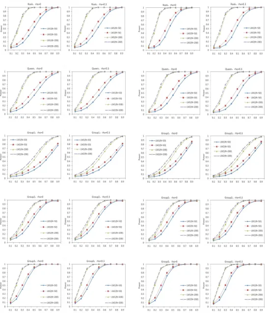
 of Zhang Jinfeng (2011) to see the improvement of the new tests in the situations where there are distribution misspecification and changes of spatial layouts. Selected Monte Carlo results are summarized in Tables 1 and Figure 1-2 and the results of other sample size such as 30, 100, 400 are available from the author upon request.

1). Z

LM test is sensitive to error distribution while our test _LMR

 not. First, as Table 1 illustrated, when spatial weight matrix is Rook contiguity and model error is normal distribution, under sample size N=50 _LMZ

 has the size close to 5%, which means their probability of refusing the null hypothesis 0

: 0

H  is among their confidential interval, while _LMR

 is a bit of higher than 5%. However, under sample size N=200, the two tests, Z

LM and LMR, have no significant difference, and their sizes are all close to 5%. When model error is log-normal distribution, Z

size N=50 while R

LM is close to 5%. However, when sample size goes to 200, the sizes of _LMZ

 (expect 0.2) and LMR are all close to 5%. But when error yields mixture-normal distribution, the two are all out of the confidential interval. Second, spatial weights matrix are Queen contiguity. While sample size N=50 for any distribution, Z

LM’s size is less than the lower limit of confidential interval while _LMR

 ’s size is close to 5%. If sample size reaches to 200, Z

LM and LMR all have correct size. These results imply that if error is not normal distribution, the performance of Z

LM under small sample size is not good. But with sample size increasing, the performance is becoming better till to the correct size while our test R

LM remains good performance. This conclusion provides some proof for the Theorem 1, which means under usual spatial weights matrix, _LMZ

 and LMR are asymptotically equivalent with sample number increasing.

2). _LMZ

 is sensitive to changes of spatial layouts while

R

LM not. As section 3 discussed, whether the correct terms of

Z

LM are negligible or not depends on the ratio of  

1 2

N

h N _.

The size results in Table 1 suggest that under the condition that error is normal distribution and spatial layout is Group contiguity, if 0.3_or 0.7

N

h N _{, the size of LM}Z

 is obviously smaller than 5% even if the sample size N goes to 200 while

R

LM_{ is close to 5%. It is the same as the case} 0.5 _or

0.5

N

h N _{. If} 0.7 _or 0.3

N

h N _{and sample size N=50,}

Z

LM(only  equal to 0.2 and 0.3) is less than the lower limit of confidential interval. When sample size N=200, only the case of  equal to 0.2 is out of the interval. However, R

LM proposed in this paper performs well and its size is close to 5%.

3). If error distribution and spatial layouts do not yield

regular assumption, _LMR

 has better size than LMZ . For example, when error is mixture-normal distribution and spatial weights matrix are Group contiguity ( 0.3 _or

0.7

N

h N _{), size of LM}Z

 is close to 2.5% under N=50 while

R

LM is 4%. When sample size goes to 200, the size of LMZ and _LMR

 is 3% and 4.3%, respectively. The case of error is log-normal distribution and Group contiguity (0.3 _or

0.7

N

h N _{) is similar to the above example. Furthermore, when}

spatial matrix are Group contiguity (0.5 _or 0.5

N

h N _{), the}

size of Z

LM is not located in the confidential interval for any

non-normal distribution, while R

LM is close to 5%. Finally, if spatial layout is Group contiguity (0.7 _or 0.3

N

h N _{), LM}Z



and R

LM all have correct size since the correct part of LMZ could be negligible.

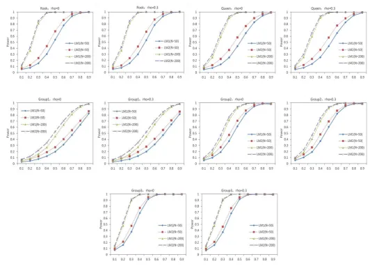
4). The power of R

LM is better than LMZ for any case. Figure 1-3 describe the power of the tests. When error is normal distribution as Figure 1 illustrated, the power of _LMR



is significantly better than Z

LM under sample size N=50, while the two have almost the same power under N=200(but

R

LM is a little bit better). It is similar to the non-normal distribution cases. For instance, when model error is log-normal distribution (Figure 3) and spatial layout is Group contiguity, the power of Z

LM is inferior to LMR with small sample size while under large sample size except the case of

0.3

 _or 0.7

N

h N _{the two tests have similar power.}

V. CONCLUSION

This paper proposes a robust LM test, _LMR

, for spatial error model, and points out that our test is asymptotically equivalent to existing tests under certain condition. Also, our test is not sensitive to error distribution and spatial layouts. Monte Carlo results provide the proof of above remarks and suggest that our test _LMR

 is better under finite sample size. For example, when spatial weights matrix are Rook or Queen contiguity, the two tests is asymptotically equivalent with sample size increasing. However, when spatial layout is Group contiguity, especially the case of 0.3_{, comparing}

with existing tests which have wrong size (smaller) for any distribution and sample size, while R

LM has the correct size. The proposed test is based on simple linear regression model, thus deriving robust tests of spatial panel data will be next step in the future.

REFERENCES

[1]. Anselin, L., (1988), Lagrange multiplier test diagnostics for spatial dependence and spatial heterogeneity [J], Geographical Analysis, 20, 1–17.

[2]. Anselin, L., (2001), Rao’s score test in spatial econometrics [J], Journal of Statistical Planning and Inference, 97, 113–139.

[3]. Anselin, L., A. K. Bera, R. Florax, and M. J. Yoon, 1996, Simple diagnostic tests for spatial dependence [J], Regional Science and Urban Economics, 26, 77–104.

[4]. Bera, A. K., and M. J. Yoon, (1993), Specification testing with locally misspecified alternatives [J], Econometric Theory, 9, 649–658. [5]. Baltagi, Badi and Yang, Zhenlin, (2010), Standardized LM Tests for

11-2010, Working Papers, Singapore Management University, School of Economics.

[6]. Burridge, P., (1980), On the Cliff-Ord test for spatial correlation [J], Journal of the Royal Statistical Society. Series B, 42, 107–108. [7]. Kelejian, H. H. and Robinson, D. P. (1995). Spatial correlation: a

suggested alternative to the autoregressive models. In: New Directions in Spatial Econometrics[C], Edited by L. Anselin and R. J. G. M. Florax. Berlin: Springer-Verlag.

[8]. Kelejian H. H. and Prucha, I. R. (2001). On the asymptotic distribution of the Moran I test statistic with applications[J], Journal of Econometrics 104, 219-257.

[9]. Lee, L. F. (2004a). Asymptotic Distributions of Quasi-maximum Likelihood Estimators for Spatial Autoregressive Models[J], Econometrica 72, 1899-1925.

[10]. Lee, L. F. (2004b). A supplement to’ Asymptotic distributions of quasi-maximum likelihood estimators for spatial autoregressive

models’ [W], Working paper , Department of Economics, Ohio State

University.

[11]. Lee, Lung-Fei, (2002), Consistency and Efficiency of Least Squares Estimation for Mixed Regressive, Spatial Autoregressive Models[J], Econometric Theory, 18, issue 02, p. 252-277.

[12]. Zhang Jinfeng, Fang Ying, (2011), Robust tests for Spatial Error Model[J], The Journal of Quantitative & Technical Economics, issue 01, p.152-160.

张进峰,方颖,. 空间误差模型的稳健检验[J]. 数量经济技术经济研 究,2011,(1), p. 152-160.

APPENDIX:PROOF OF THE THEOREM

To prove the theorems, we need the following lemmas.

Lemma L1 (Lee, 2004a, p.1918): Let V _{be an} N1

random vector of i.i.d. elements with mean zero, variance _2

, and finite excess kurtosis 4

4 3

v

    . Let A _and B _be N

dimensional square matrix with  aii and  bii are the

diagonal elements of A _and B _{, respectively. Then:}

  2  

'

E V AV tr A _,   2  

'

E V BV tr B _and

 

















 





   





4 2 4 2

4

4 2 2

4 4

4 4

' 3 '

'

' , ' 3 '

'

ii i v i ii

ii ii i v i ii ii

Var V AV a tr AA A a tr AA A

Cov V AV V BV a b tr AB AB a b tr AB AB

                           

Lemma L2 (Lemma A.9, Lee, 2004b): Suppose that the

elements of the NK _matrix X_{are uniformly bounded; and}

1

limN N X X'



 exists and is nonsingular. Then the projectors

 1

' '

X X X  X _and M I X X X ' 1X' _{are uniformly bounded in}

both row and column sums. Suppose that A _{represents a}

sequence of NN _{matrices that uniformly bounded in both}

row and column sums. Then

       

       

   





 

 

  









 





 



 

2 2

2 2 2

1

' ' 1

1

' ' ' 1 .

i tr MA tr A O ii tr A MA tr A A O iii tr MA tr A O

iv tr A MA tr MA A tr A A O

 

 

 

  

Furthermore, if

 

1

ij N

a O h _{for all} i _and j_{, then}

     

 

     

 

2 2 1

2 2 1 1 1 n n n ii n

i ii i

v tr MA tr A O nh vi MA a O h

             

where  MAii are the diagonal elements of MA, and aij the

diagonal elements of A_.

Lemma L3 (Lee, 2004a, p1918): Suppose that A _{is a}

square matrix with its column sums being uniformly bounded and elements of the NK _matrix Z _{are uniformly bounded.}

Then,

 

1 n Z AV' O 1 _{. Furthermore, if the limit of} Z AA Z N' '

exists and is positive definite, then







2



1 ' D 0, lim ' '

n

N Z AVN  Z AA Z N .

Lemma L4 (Kelejian&Prucha, 1995; Lee, 2002): Let  A

and  B _{be two sequence of} NN _{matrices that are}

uniformly bounded in both row and column sums. Let C _be

a sequence of comfirmable matrices whose elements are

uniformly

 

1

N

O h _{. Then}

 i _{the sequence} AB _{are uniformly bounded in both row}

and column sums.

 ii _{the elements of} A _{are uniformly bounded and}

   

tr A O N _{, and}

 iii _{the elements of} AC _and CA _{are uniformly}

 

1

N

O h _.

Proof of theorem 1: First, we note that

 

 

2 1

2 1 1 1

1 1 1 ' ' ' ' N N

e W e S e W S I e

εM W S I Mε

εPε



  

 



(A.1)

Under _H0

 and Assumption A1, Lemma L1 is applicable to ε'Pε _{, which gives} 2  

' 0

EεPεtr P  _and

  4 2 4  

 

2 4 

12 13 1

' Ni ii '

Var εPε _p  _tr AA tr A _  S S _{. Letting}

0 1

2 1

P W n S I _{, we have PMP M}0 _{. By Lemma L2} i _and

Assumption A2, tr MW 2  O1 which gives

 

1 1

1

NS O N



 _.

Hence, the elements of _P0 _{are of uniform order}

 

1

N

O h _.

Under Assumption A3, M _{is uniformly bounded in both row}

and column sums (Lemma L2). It follows that the matrix of

P _{are uniformly bounded. Thus, the generalized central limit}

which shows that ε'Pε _{is asymptotically normal, or}

equivalently,

 



4



12 13

' D 0,

εPεN  S S _(A.2)

Second, we note that









2 1 1 1

1 2 1 1 1

1 1

' ' ' '

' '

e W y S e W A Xβ e W A ε e n S I e

εM W A Xβ εQε

   



   

  (A.3)

Under 0

H and Assumption A1, Lemma L1 is also applicable to the above equation, then



1



2  

1

' ' 0

E_εM W A X β εQε_tr Q  _and



1



4 

1 22 23 24

' '

Var_εM W A X β εQε_ S S S _{. Letting} 0 1 1

1 2

Q W An S I _,

we have 0

QMQ _{. By Lemma L2} i _{and Assumption A2,}

 1  1

tr MW O _{which gives} 1

 

1 2

NS O N



 _{. Thus, the elements of}

0

Q _{are of uniform order} O h

 

N1



. Under Assumption A3, the

elements of Q _{are of uniform order}

 

1

N

O h _{and the row and}

column sums of the matrix Q _{are uniformly bounded.}

Therefore, the ε'Qε _{is asymptotically normal based on the}

generalized central limit theorem of linear-quadratic form of

Lee (2004a),



4 



22 23

' D 0,

εQεN  S S _.

Third, by Assumption A2 and A3, it shows that 1 1

W A X β

is uniformly bounded and M _{is uniformly bounded in both}

row and column sums. Hence, by Lemma L3, we have







1





2



1 24

1 _{N W A X} _β '_MεD _N 0,_{S N}

. Thus,



1



1

' '

εM W A X β εQε _is

asymptotically normal, or equivalently,







 



2 1 4 4

1 2 1 22 23 24

' ' ' 0,

e W yS εM W A X β εQεN  S S S (A.4)

By A.1, A.3 and Lemma L1, we have

 





  

 





  





     

2 2 1

2 1 1 2 1

4 32 33

1

2 2

2 1 32 33 22 23 24 1 2

2 1

4

12 13 32 33 22 23 24

' , ' ' ' '

' '

' '

Cov e W e S e W y S E εPε εMW A Xβ εQε E εPε εQε

S S

Var e W e S S S S S S e W y S S S S S S S S

                     _  _             _{     }         _      _ (A.5)

With A.2, A.4 and A.5, we have



2



  1



2



2 1 32 33 22 23 24 1 2

' '

e W eS S S S S S  e W yS _is

asymptotically normal, or equivalently,





  





       

1

2 2

2 1 32 33 22 23 24 1 2 1 2

2 1

2

12 13 32 33 22 23 24

' '

0,1

e W e S S S S S S e W y S N S S S S S S S

                  _{    }      (A.6)

Now, it is easy to show that 2 p 2

 

  _, p

 

  _and

24 24

p

S S _{by replacing} 2



 ,  and S24 with 2



 ,  and

4

S _{, respectively. Slusky}’_{s theorem suggests that the square of}

A.6 yields chi-square distribution with one degree of freedom. This finished the poof of Part (i).

For Part (ii), it suffices to show that S1O 1 ,



1



 

2 1 1

S tr W A O _and S24~S24 by Lemma L2 i , where ~

stands for ‘asymptotic equivalence’. Following from Lemma L2, we have

 

















       

   

1 1

2 1 2 1

1 2 2

2 2 1 2 1

2 2

' '

' 2 1

' 1

tr PP tr M W n S I M M W n S I M tr W W n S tr MW n S tr I O tr W W O

       _   _          





























     





 

1 1 1 1

1 2 1 2

1 1 1 1 2 2

1 1 2 1 2

1 2 1 1

' '

' ' 2 1

' 1

A A

tr QQ tr MW A M n S I MW A M n S I tr W A W A n S tr MW A n S tr I O tr S S n tr W A O

                      





























         

1 1 1

2 1 1 2

1 1 1 1 2

2 1 1 1 2 2 1 2

2

' '

' 1

' 1

A

tr PQ tr M W n S I M MW A M n S I

tr W W A n S tr MW A n S tr MW n S S tr I O tr W S O

           _   _         

Then tr PP tr W W 2 2O 1 ,    





  2 1 1

1

A A N

tr QQ tr S S  tr WA O _,

   2 A  1

tr PQ tr W S O _.Hence, S13~tr W W 2 2'W W2 2T22 ，

  2



 



2

2 1

23 24~ AA n A A ' A

S S T  tr S _ S Xβ M S Xβ J_{ } and

 

33~ 2 A 2' A 2A

S tr W S W S T _{. Therefore, when} 0 , LMR is asymptotically equivalent to _LMZ

TABLE 1: SIZE OF THE TESTS

W 

Standard Normal Distribution Mixture-Normal Distribution Log-Normal Distribution

N=50 N=200 N=50 N=200 N=50 N=200

Z

LM_{ LM}R

 LMZ LMR LMZ LMR LMZ LMR LMZ LMR LMZ LMR

Rook

0.0 0.0506 0.0565 0.0468 0.0486 0.0459 0.0500 0.0590 0.0582 0.0383 0.0487 0.0467 0.0543

0.1 0.0466 0.0555 0.0512 0.0539 0.0478 0.0486 0.0646 0.0650 0.0414 0.0485 0.0463 0.0479

0.2 0.0440 0.0570 0.0459 0.0495 0.0431 0.0524 0.0614 0.0611 0.0393 0.0476 0.0427 0.0483

0.3 0.0505 0.0579 0.0476 0.0504 0.0505 0.0522 0.0644 0.0639 0.0393 0.0483 0.0484 0.0530

0.4 0.0450 0.0540 0.0476 0.0504 0.0491 0.0474 0.0642 0.0651 0.0398 0.0460 0.0495 0.0511

0.5 0.0502 0.0570 0.0500 0.0496 0.0491 0.0533 0.0615 0.0593 0.0393 0.0478 0.0464 0.0492

Queen

0.0 0.0405 0.0537 0.0445 0.0459 0.0393 0.0461 0.0499 0.0527 0.0376 0.0530 0.0473 0.0500

0.1 0.0405 0.0567 0.0492 0.0529 0.0401 0.0478 0.0481 0.0552 0.0383 0.0481 0.0433 0.0488

0.2 0.0398 0.0530 0.0505 0.0479 0.0390 0.0479 0.0500 0.0519 0.0346 0.0494 0.0423 0.0533

0.3 0.0420 0.0516 0.0471 0.0488 0.0410 0.0439 0.0545 0.0552 0.0330 0.0497 0.0454 0.0479

0.4 0.0395 0.0520 0.0479 0.0521 0.0433 0.0471 0.0522 0.0560 0.0371 0.0544 0.0442 0.0550

0.5 0.0414 0.0565 0.0460 0.0487 0.0370 0.0505 0.0516 0.0540 0.0345 0.0477 0.0443 0.0496

Group

0.3



0.0 0.0255 0.0425 0.0349 0.0497 0.0249 0.0409 0.0300 0.0404 0.0251 0.0414 0.0317 0.0431

0.1 0.0222 0.0405 0.0330 0.0486 0.0228 0.0408 0.0294 0.0433 0.0227 0.0394 0.0304 0.0436

0.2 0.0253 0.0420 0.0309 0.0500 0.0245 0.0393 0.0302 0.0414 0.0217 0.0366 0.0306 0.0439

0.3 0.0264 0.0432 0.0337 0.0534 0.0259 0.0390 0.0317 0.0449 0.0241 0.0372 0.0266 0.0435

0.4 0.0231 0.0411 0.0325 0.0513 0.0238 0.0383 0.0310 0.0436 0.0243 0.0385 0.0295 0.0423

0.5 0.0263 0.0404 0.0299 0.0511 0.0239 0.0374 0.0282 0.0406 0.0267 0.0424 0.0282 0.0458

Group

0.5



0.0 0.0336 0.0471 0.0363 0.0497 0.0350 0.0434 0.0427 0.0471 0.0347 0.0480 0.0409 0.0504

0.1 0.0359 0.0497 0.0397 0.0486 0.0343 0.0467 0.0415 0.0456 0.0346 0.0486 0.0396 0.0491

0.2 0.0338 0.0517 0.0342 0.0500 0.0339 0.0469 0.0406 0.0451 0.0330 0.0472 0.0389 0.0481

0.3 0.0333 0.0496 0.0404 0.0534 0.0347 0.0502 0.0413 0.0492 0.0325 0.0479 0.0393 0.0492

0.4 0.0347 0.0460 0.0408 0.0513 0.0376 0.0444 0.0385 0.0465 0.0326 0.0481 0.0339 0.0459

0.5 0.0331 0.0504 0.0373 0.0511 0.0357 0.0471 0.0402 0.0441 0.0332 0.0459 0.0382 0.0506

Group

0.7



0.0 0.0460 0.0532 0.0470 0.0494 0.0464 0.0520 0.0519 0.0564 0.0417 0.0542 0.0474 0.0507

0.1 0.0438 0.0486 0.0460 0.0534 0.0472 0.0507 0.0581 0.0597 0.0426 0.0485 0.0450 0.0493

0.2 0.0408 0.0502 0.0430 0.0463 0.0432 0.0516 0.0584 0.0558 0.0433 0.0524 0.0439 0.0520

0.3 0.0427 0.0562 0.0480 0.0524 0.0509 0.0544 0.0549 0.0611 0.0446 0.0533 0.0472 0.0530

0.4 0.0462 0.0550 0.0455 0.0518 0.0473 0.0516 0.0581 0.0579 0.0453 0.0518 0.0477 0.0533

[image:10.595.24.565.47.685.2]

Figure 1. Power of the tests (standard normal (left two columns) and mixture-normal(right two columns) distribution): LM1:_LMZ

[image:11.595.39.572.54.436.2]

Figure 2. Power of the tests (log-normal distribution) : LM1:_LMZ