Approximating correlated defaults

Approximating correlated defaults

Rosenthal, Dale W.R.

University of Illinois at Chicago

15 February 2012

DALE W.R. ROSENTHAL

Abstract. Modeling defaults is critical to risk management as well as

pricing debt portfolios and portfolio derivatives. In the recent financial

crisis, multi-billion-dollar losses resulted from correlated defaults that

were improperly modeled. This paper proposes statistical

approxima-tions which are more general than those used previously, follow from an

intensity-based risk-factor model, and allow consistent parameter

esti-mation. The parameters imply an approximating portfolio of

indepen-dent, identical-credit loans and characterize both average credit quality

and default-relative diversification (aka the “diversity score”). Unlike

previous approaches, these metrics are derived jointly from theory. The

approach addresses weaknesses in the typical diversity score-based

meth-ods by allowing for fatter tails as well as loans differing in size and credit

quality. The approximations may also be used to model complete

port-folio default and help set capital adequacy requirements. An example

shows how to estimate the approximating portfolio.

(JEL: G13, G12, C16, G33)

In the financial crisis of 2008–2009, US households lost about $11

tril-lion in wealth and structured debt securities alone suffered impairments of

over $1.5 trillion.1 _{Many loan portfolios experienced high numbers of}

corre-lated defaults: defaults at an accelerated rate and clustered in time. This

Helpful comments were provided by Per Mykland, Michael Wichura, and participants at the SoFiE Geneva, Peking Guanghua QMBA, and Oakland credit analysis conferences. Financial support from the National Science Foundation under grants DMS 06-04758 and SES 06-31605 is gratefully acknowledged.

Address correspondence to Dale W.R. Rosenthal, Department of Finance, University of Illinois at Chicago, 601 S. Morgan St (MC 168), Chicago, IL 60607; e-mail: [email protected]. 1_{Statistics on the scope of the crisis and the effect on structured products are well}

docu-mented in Financial Crisis Inquiry Commission (2011) and Tunget al._(2011).

correlation was greater than predicted by typical methods such as Schorin

and Weinreich (1998). One of the causes and magnifiers of the crisis noted

by the Financial Crisis Inquiry Commission was the increased correlation

of risky assets. In particular, the US Federal Reserve’s Troubled Asset

Re-lief Program and Term Asset-Backed Securities Loan Facility programs were

targeted at assets which had been affected by a larger-than-expected number

of concurrent defaults.

Modeling correlated defaults well is of particular importance because of

the real effects of defaults. Many of these effects were seen in the recent

financial crisis. Financial firms withdrew funding liquidity from world

mar-kets; financial and non-financial firms failed due to the loss of funding; and,

unemployment increased while tax revenues decreased. Many investors not

directly affected by these troubles were affected by the increased market

volatility. Some investors rebalanced their portfolios at a time when doing

so was costly. Other investors chose not to fund risky ventures which further

suppressed job growth.

Since defaults are so destructive, lenders often manage default risk by

creating portfolios of loans. These portfolios may be tranched or split into

portfolio credit derivatives such as collateralized debt obligations (CDOs).

Default risks of portfolios, tranches, or other derivatives may also be hedged

with credit default swaps (CDSs). A primary concern for any portfolio,

however, is risk correlations. Two approaches dominate the modeling of

default: structural models of firm assets and liabilities and reduced-form

models of default intensities.

This paper shows how the assumptions behind some reduced-form

ap-proaches may be too restrictive. We propose apap-proaches that relax these

assumptions to find default-approximating portfolios. We then show how

quality of a loan portfolio. The source of these two measures is more robust

than many reduced-form methods because the assumptions are weaker. The

measures also better capture the tail risk of default times.

To get at the correlation of such defaults, we propose modeling the time

to loan default as an idiosyncratic component which interacts with shared

systematic components (risk factors). Since shared risk factors lead to

de-fault correlation, we explore approximating expansions for the distribution

of correlated default times. The expansions imply approximating portfolios

of independent, identical-credit loans.

The parameters of these approximations have direct economic meaning

for the approximating portfolios: they measure both default-relative

diver-sification of a correlated loan portfolio and aggregate credit quality. The

default-relative diversification is measured via an iid-equivalent loan count

and yields a theoretically-derived maximum likelihood version of Moody’s

KMV’s diversity score.2 _{One contribution of this paper is to derive the}

diversity score jointly with the average credit quality so that the two are

consistent. Furthermore, one of the approximating expansions has a form

which is mathematically concise and theoretically novel.

1. Thinking About Default Times

Since we can think of the time to loan default as random, it makes sense

to ask when such a default is more likely to occur. The structural

model-ing approach assumes that default happens at a random time determined

by the stochastic evolution of a firm’s assets (and perhaps liabilities) with

2_{An explanation of a common approach to calculating the Moody’s KMV diversity score is}

default occuring when some barrier is hit by the asset process. The

reduced-form intensity-based approach does not model the firm and instead assumes

defaults of individual loans happen stochastically at some rate.

If we observe a firm’s assets and the liability-dependent default barrier,

we may model default via structural models such as in Merton (1974), Black

and Cox (1976), and Leland and Toft (1996). Were we to observe these data

for multiple firms, we could use asset correlations with a default barrier to

study default correlation as in Zhou (2001). Giesecke (2006), however, noted

that we often cannot directly observe firm assets and that this leads us to

use an intensity-based, reduced-form modeling approach.

Reduced-form models can be traced back to theory in Erlang (1909) which

modeled the answering delay of busy operators as exponentially distributed.

Jarrow and Turnbull (1995) first suggested the modeling of bond default

times as exponentially distributed. Jarrow et al. (1997) modeled default

times of many credit ratings with Markov switching of bonds among credit

ratings; and, Banasiket al.(1999) briefly considered exponential or Weibull

default times. Collin-Dufresneet al. (2004) modeled default times as

expo-nential with random intensities and discuss modeling a two-loan CDO.

Modeling correlated defaults is more complex and thus came later.

Jar-row and Yu (2001) used the JarJar-row-Turnbull model to study default by two

firms with bond cross-holdings; and, they note that for more firms “working

out these distributions is more difficult.” This complexity explains the

popu-larity of reduced-form approaches. Duffie and Gˆarleanu (2001) decomposed

a firm’s (exponential) default rate into systematic and idiosyncratic

exponentially distributed defaults correlated by a joint distribution with

ex-ponential marginals and a singular “spine.”3 _{Duffie et al. (2009) analyzed}

which random variables affect the default intensity process using a linear

model.

The approximations used here follow from theory in Edgeworth (1883).

Patnaik (1949), Cox and Reid (1987), and McCullagh (1987) discussed

sim-ilar approximations; and, Cox and Barndorff-Nielsen (1989) approximated

a weighted sum of Exp(1) variables with a gamma density and hinted at a

possible expansion. However, none of those approaches use approximations

of the form here.

2. Reduced-Form Model and Approximation Consistency

We start with a reduced-form model that assumes the time to default for

one loan is exponentially or nearly gamma-distributed.4 The gamma

dis-tribution has not generally been used in the reduced-form default-intensity

literature. However, if other random events alter the default rate, the actual

distribution of defaults may well be gamma-distributed (as is shown later).

Furthermore, the gamma is a less restrictive distributional assumption since

the exponential distribution is a special case of the gamma (with 1 degree

of freedom).

We assume multiple possible events affect the rate at which a borrower

defaults. One event is idiosyncratic to the borrower; others are related to risk

factors. These risk events interact with the idiosyncratic event. For example,

defaults may increase with rising interest rates, tightening credit standards,

or an economic downturn. The possibility that loans may share risk factors

3_{This construction is the same as the failure-time distribution first studied by Marshall}

and Olkin (1967). Simultaneous defaults are theoretically problematic since they imply a singular component of the joint distribution which breaks the assumptions of most modeling approaches. For this reason, we do not follow this approach.

4_{Default may be censored, including by loan maturation. This does not challenge the}

yields positively-correlated default times for multiple loans. Portfolios of

many loans would then behave like portfolios of fewer loans.

The assumption of risk factors affecting default intensities is not new;

others have used affine models to explore shared risk factors. While affine

models are simpler, they can be problematic if used to model bonds of

differ-ing credits. Affine models imply that bonds of differdiffer-ing credit experience the

same additive change in their default rate with respect to a risk factor. For

example, a AAA-rated bond in recession would default at a rateλAAA+γ

and a B-rated bond would default at a rateλB+γ where λB > λAAA.

In-stead, we assume that the default rate changes by a multiplicative factor

(e.g. δλAAA and δλB) with respect to a risk factor. Further support for

using a non-affine model comes from Daset al. (2007) who found clustering

beyond that suggested by an affine model.

Unfortunately, working with a non-affine model is more difficult than

working with an affine model. However, if we can find a default-approximating

portfolio of independent identical-credit loans, we can then model the

dis-tribution of portfolio defaults. To help find this portfolio, we focus on the

distribution of the average time to default.5 While we would prefer to work

with the default time distribution, working with the distribution of the

av-erage allows us to prove asymptotic consistency. This approach was also

used by Schorin and Weinreich (1998).

2.1. Reduced-Form Model. We begin by setting up notation. Let:

k = number of risk factors/possible risk events;

ℓ = number of loans/possible idiosyncratic default events;

Xi = delay before an event i, i∈ {1, . . . , ℓ+k};

5_{Finding the average default time for a portfolio involves adding multiple exponential}

λi = rate parameter characterizing delay Xi;

δj = rate multiplier of λi∈{1,...,ℓ} after risk eventj ∈ {1, . . . , k};

Yi = time to default for loan i∈ {1, . . . , ℓ}; and,

Ft = filtration encapsulating information known up to time t.

The model assumes event times are exponentially distributed. For each

loani_{∈ {}1, . . . , ℓ_}, the rate parameterλiimplies an idiosyncratic probability

of default in a given year and thus a certain credit quality. For each risk

factorj _{∈ {}1, . . . , k_}, the rate parameterλℓ+j implies a probability of a risk

event occurring in a given year andXℓ+j is the time of that occurrence.

To model default times, we assume a relationship of events for each loan.

First, loans default at their idiosyncratic default rates λ_{i∈{1,...,ℓ}}. Second,

some loans may be exposed to a risk factor j and undefaulted when a risk

factor event occurs. The idiosyncratic default rate of these loans accelerates

to δjλi after that risk event. For example, homeowners might default at a

certain rate but at twice that rate after the economy enters a recession.

2.2. Homogenous, Independent Loans. We start by considering loans

with no risk factors and only idiosyncratic propensities to default. This

approach helps develop the case where loans have shared risk factors.

For independent loans of equal credit quality (λi∈{1,...,ℓ} =λ), the average

default time ¯Y = 1_ℓPℓ_i=1Xi is a Gamma(ℓ, ℓλ) random variable. For loans

of unequal size, let wi >0 be the portfolio weight of loani. If larger loans

are more likely to default, notional weighting may drive the average default

time to being gamma-distributed.

Theorem 1. (When Default Rates Scale with Loan Size) Ifℓ >1:

1) Xi

indep

∼ Exp(λi) ∀ i∈ {1, . . . , ℓ >1}; and,

2) there exist weights 0< wi <∞ such that λi/wi =ℓλ,

Proof. The mgf exists in a neighborhood aboutt = 0 and is integrable for

ℓ > 1, identifying the distribution. _MY¯(t) = Qℓ_i=1λ λi

i−wit =

Qℓ

i=1 ℓλℓλ−t,

which is the mgf for a Gamma(ℓ, ℓλ) random variable.

If the λi/wi quotients are not equal, we essentially have heterogeneous

rates. Since the mgf for a sum of independent random variables is the

product of the individual mgf’s, we get the mgf and cumulant generating

function (cgf):

M_Y¯(t) =

ℓ

Y

i=1

λi

λi−wit

,

(1)

K_Y¯(t) =

ℓ

X

i=1

(logλi−log(λi−wit)),

(2)

and the first four cumulants of ¯Y: (κ1, κ2, κ3, κ4) =Pℓi=1(wλii,

w2

i

λ2

i

,2w3i

λ3

i

,6w4i

λ4

i

).

Since the mgf and cgf depend on the individual rates, we must find the

density explicitly for each problem instance. This can be cumbersome for

portfolios of many loans.

2.3. Reduced Form Consistency. We may progress further if we assume

nothing about independence, the λi’s, nor the number of risk factors k.

Instead, we approximate the density of the average default time ¯Y.

Edge-worth (1883, 1905, 1906) suggests expanding about a base density to get an

approximate density.

To more easily express event times, we letX_(j) be the order statistics for

the risk event times Xℓ+1, . . . , Xℓ+k such that X(1) ≤ · · · ≤ X(k). We also

letδ_(j) be the rate acceleration parameter forX_(j)and set k_i∗ to be the time

of the most recent risk event which affected loani:

k∗_i = arg max

j

By the memoryless property of the exponential distribution, the timeYi

to default on loan i_{∈ {}1, . . . , ℓ_} may be written as a sum of a rate-changed

idiosyncraticXi and systematic Xj∈{ℓ+1,...,ℓ+k}’s. This allows us to express

the default timeYi of loan ias

Yi|Ft= k∗

i

X

j=1

(X(j)−X(j−1)) +

Xi−X(k∗

i)

Qk∗

i

j=1δ(j)

= Xi−X(k∗i)

Qk∗

i

j=1δ(j)

+X(k∗

i)

(4)

L = _Qk∗Xi

i

j=1δ(j)

+X_(k∗

i).

(5)

Simulation of these random variables is explained further in Section 4.1.

To approximate correlated loan portfolios, we must ensure Edgeworth

expansions may be used. The following proof shows consistency for the

mean of the previously-outlined construction of default times:

Theorem 2. (Consistency for Exponentials Correlated by Risk Factors)

Assume the following hold:

1) Xi’s are partitioned by index sets: one independent _S¯ (idiosyncratic

risk factors) and many singular _S1, . . . ,Sk (systematic risk factors).

2) If loan i _{∈ {}1, . . . , ℓ_} is exposed to risk factor j _{∈ {}1, . . . , k_}, then

i_{∈ Sj}.

3) At least two of these index sets are non-empty.6

4) Xi’s in the independent index set (Xi∈S¯’s) are independent.

5) Xi’s belonging to different index sets are independent. (Thus all risk

factors and idiosyncratic risks are independent.)

6) ¯Y = 1_ℓ Pℓ_i=1Yi.

7) Xi∼Exp(λi) ∀ i∈ {1, . . . , ℓ+k}.

6_{Were this not true, a risk event could cause all loans to immediately default. That would}

yield a non-zero probability ofX_i=X_i′ fori6=i′. Such a singularity would prevent us

Then Edgeworth expansions are consistent estimators of the Y¯ density.

Proof. By assumption 1, we may put XSj := Xi∈Sj with rate λSj for all

j_{∈ {}1, . . . , k_}. We then rewrite ¯Y as

¯

Y_|FT = 1

ℓ

 X

i∈S¯

Xi

Qk j=1δ

I(i∈Sj)

j

+_|S1|XS1+. . .+|Sk|XSk

  (6) = 1 ℓ  X

i∈S¯

X_i∗+_|S1|XS1 +. . .+|Sk|XSk

 ,

(7)

whereX_i∗is a rate-changed exponential random variable with rateλiQkj=1δ

I(i∈Sj)

j .

Since XS1, . . . , XSp are exponentially distributed, we can rewrite|Si|XSi

as an exponential random variable X_S∗_i with rate λ_S∗_i =λSi/|Si|. Thus we

get ¯Y =P_i∈S¯X_i∗+Pk_i=1X_S∗_i.

This is a sum of independent, non-identically distributed constituents.

This meets the regularity conditions in Feller (1971) since ¯Y has finite higher

moments and the characteristic functionφ_Y¯(t) is integrable for m >1.

Corollary 1. (Individual Default Times Are Nearly Gamma-Distributed)

Under the assumptions above, if a loan is exposed to at least one systematic

risk factor, the default time for that single loan is nearly gamma-distributed

(and possibly not exponentially distributed).

Proof. Given the proceeding proof, we need only note that:

Yi=

Xi

Qk j=1δ

I(i∈Sj)

j

+

k

X

j=1

I(i_{∈ Sj})XSj

(8)

If there is at least one systematic risk factor to which loaniis exposed, then

the sum meets the regularity conditions outlined above and the

3. Approximation Forms

With consistency assured, we investigate three asymptotic

approxima-tions: (1) normal Edgeworth expansions; (2) gamma Edgeworth expansions;

and, (3) a combination of the above (“m´elange”).7

3.1. Normal Edgeworth Expansions. Most Edgeworth expansions use

a normal base density and expand about the normal density yielding

mul-tiplicative correction terms involving Hermite polynomials. This creates a

distribution approximation with support over all ofR. We begin with such

an expansion by matching the first two cumulants:

f_Y¯(y) = φ√(z)

κ2

1 +κ3(z 3_−3z)

6pκ3₂ +

κ4(z4−6z2+ 3) 24κ2₂

+ κ

2

3(z6−15z4+ 45z2−15) 72κ3

2

+O(ℓ−3/2) (9)

where z = (y₋κ1)/√κ2. While the correction terms allow us to match

skewness and kurtosis, the tail decay is of order e−z2 which may be

prob-lematic as discussed in Duffie and Gˆarleanu (2001).

3.2. Gamma Edgeworth Expansions. While most Edgeworth

expan-sions are based on the normal density, Section 2 suggests the default time

density might be close to a gamma density. If we use a gamma base density

and expand about that, the resulting correction terms are binomial sums

of other gamma densities differing only in the degrees of freedom. This

approach also has the structural advantage of assigning zero probability to

negative default times.

To clarify the results, we let:

7_{Approximation of the log-density, was also explored. Such forms are non-negative but}

γℓ,λ(y) = the Gamma(ℓ, λ) pdf if ℓ >0,else 0; and,

γ_ℓ,λ(k)(y) = the k-th bounded derivative of γℓ,λ(y),else 0

=λk

k

X

j=0

(₋1)k−j

k j

γℓ−j,λ(y)Iℓ−k>0.

Thus γ_ℓ,λ(k)(y) = 0 for all negative ℓ₋k. This upholds the regularity

condition of a bounded k-th derivative as in Feller (1971), page 538.

We recall the Gamma(ℓ, λ) cumulants and match the first two, implying

ˆ

ℓ =κ2₁/κ2 and ˆλ =κ2/κ1 for estimates of the effective ℓ and λ. This and

the preceding derivatives yield:

f_Y¯(y) =γ_ℓ,ˆˆ_λ(y) +

κ3ˆλ3−2ˆℓ 6

3

X

j=0

(₋1)3−j

3

j

γ_ℓˆ_−j,λˆ(y)

+κ4ˆλ 4_−6ˆℓ 24

4

X

j=0

(₋1)4−j

4

j

γ_ℓˆ_−j,λˆ(y)

+(κ3λˆ

3_−2ˆℓ)2 72

6

X

j=0

(₋1)6−j

6

j

γˆ_ℓ−j,λˆ(y) +O(ℓ−3/2), (10)

assuming that ˆℓ_≥7 to meet the aforementioned regularity condition.8

Note that the expansion has a pleasingly simple form: binomial sums of

other gamma densities. That the expansion takes this form is an elegant

and novel result. We know of no other Edgeworth expansion (apart from

the typical normal-based form) that has such a concise and easily-expressed

form. Since we have shown that default times are likely to be well

approxi-mated by a gamma distribution, this expansion also gives us the machinery

to find that approximation.

8_{We can relax this to just ˆℓ≥4 with an error bound of onlyO(ℓ}−1_{) if we drop the last}

The correction terms allow us to match skewness and kurtosis (as in the

normal expansion). The tails are fatter with decay of order e−z_{. These}

features help handle concentration risk and reduce the underestimation of

tail risk discussed in Duffie and Gˆarleanu (2001) and problematic in the

Schorin and Weinreich (1998) method, for example. For risk managers, this

model more effectively captures tail risk.

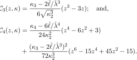
3.3. A Combination of Expansions (M´elange). We might instead

com-bine the preceding approaches: a base density thought to be close to the

true density, but coupled with correction terms from the normal density.

This approach allows for mathematially tractable correction terms and is

recommended by Cox and Barndorff-Nielsen (1989). Since the term

“com-bination” is too prevalent to refer to this approach alone and “mixture” is

used in other contexts, we dub this approach a “m´elange” for clarity and

convenience.

One possible m´elange uses a Gamma(ℓ, λ) base density and normal-derived

correction terms. This eliminates concerns about correction terms not

sat-isfying regularity conditions if ˆℓis too small; however, it assigns some small

probability to negative times.

f_Y¯(y) =γ_ℓ,ˆˆ_λ(y) +

φ(z)

√_κ

2

withz= (y₋κ1)/√κ2 as before and

C3(z, κ) =

κ3−2ˆℓ/λˆ3 6pκ3₂ (z

3

−3z); and,

C4(z, κ) =

κ4−6ˆℓ/λˆ4 24κ2

2

(z4₋6z2+ 3)

+ (κ3−2ˆℓ/ˆλ 3₎2

72κ3 2

(z6₋15z4+ 45z2₋15).

This expansion also has fatter tails (e−z decay, if the correction terms are

used) like the preceding gamma-based expansion.

4. Evaluating the Approximations

Having developed the theory, we can explore how well these expansions

approximate the average default time density for CDO tranches. Since

gamma Edgeworth regularity conditions may not hold or the expansion may

be negative, we also examine the base gamma density with no correction

terms.

The CDO setup is consistent with information in Lucas (2001) and Fender

and Kiff (2004): an underlying portfolio of 200 equal-sized loans. Each loan

has a different rate of default, chosen to equally cover a range of log-default

rates. The CDO trust is divided into three tranches, with defaults allocated

to the lowest still-extant tranche (Table 1).

Tranche # Loans Percent

A 150 75%

Mezzanine 40 20%

Equity 10 5%.

Table 1. Tranche structure for a 200-loan CDO with three

While this CDO setup differs from later standardization on 125-loan

CDOs, the results here would be even stronger for a 125-loan CDO. For a

125-loan CDO, limiting asymptotic approximations would be less accurate

and thus would make these (large deviation) expansions perform relatively

better.

Default correlations are induced by the possibility of one (i.e.k= 1) rare

systematic risk event such as a sharp economic downturn at timeXℓ+1. Each

loaninot in default experiences accelerated default: the remaining time to

default is divided by a factor δ1. (By the memoryless property, Theorem 2

still applies.9)

We assume a range of equally spaced default rates. Since the

log-default rates are equally spaced, this setup is more difficult to handle than

if that range supported a modal distribution of log-default rates. These yield

average (idiosyncratic, unshocked) default times of 5–20 years with a skew

toward better credits: λi = 10i/200/20 for i ∈ 1, . . . ,200. The systematic

shock occurs at a rate λℓ+1 = 0.05, implying a mean time-to-shock of 20

years.10 Since the one-time shock is serious, the default time acceleration

used isδ1 = 5. These are equivalent to a portfolio of B–C-rated loans which

become C–D-rated during a recession.

4.1. Generating Risk Factor-Correlated Defaults. 200,000 simulated

loan portfolios were created using Algorithm 1. The simulations yielded

de-fault times for each loan. Cumulants of those dede-fault times were calculated,

which implied parameters for the expansions. The target density was then

9_{By memorylessness, shocked loans default atX}

ℓ+1+Xi′ for a risk event at timeXℓ+1∼ Exp(λℓ+1),Xi′∼Exp(δλi).

plotted along with the approximations, and goodness-of-fit measures were

calculated.

The simulation method uses the memoryless property of the exponential

distribution. Specifically, we use the fact that the distribution of the time

remaining to default is conditionally independent of a stopping time. This

property implies that the time remaining has the same distribution as the

original default time (given the information at time 0), and allows us to

efficiently reuse idiosyncratic random variates.

Algorithm 1. (Risk Factor-Correlated Default Times)

1) Generate idiosyncratic default times: X˜_{i∈{1,...,ℓ}}indep_∼ Exp(λi).

2) Generate systematic shock time: X˜ℓ+1 ∼Exp(λℓ+j).

3) For i= 1 to ℓ, process each loan.

(a) If X˜i>X˜ℓ+1:

Accelerate remaining default time in affected loans.

1: Set X˜i := ( ˜Xi−X˜ℓ+1)/δ1.

2: Combine time periods:

Xi = ˜Xi+ ˜Xℓ+1.

(b) Otherwise: Xi = ˜Xi.

Appendix A explains how to do this sort of a simulation in a setting with

multiple risk factors, which is a bit more involved.

4.2. Example: CDO Equity Tranche with Major Shock. The average

default time of a CDO equity tranche can be modeled as a mean of correlated

exponential random variables. The equity tranche of a CDO is the riskiest

and most likely to be affected by correlated defaults. Thus we focus on

approximating the equity tranche under the possibility of a major shock,

The average default time is the sample mean ( ¯Y) of the ten smallest

generated default times. Simulated ¯Y’s yielded the sample cumulants of

(ˆκ1,κˆ2,κˆ3,ˆκ4) = (0.142,2.583×10−3,1.018×10−4,6.458×10−6) which

im-plied gamma parameters of ˆλ= 55.12 and ˆℓ= 7.849.

The average simulated default time is about two months; and, the

esti-mated diversity score (iid loan count) is 7.8. This implies that the shared

systematic risk factor causes a reduction in default-relative diversification of

nearly one-quarter. Further, we can think of the equity tranche as having

default behavior like a portfolio of 7.8 loans each with an annual probability

of default of 1₋e−55.12 _≈ 1 (F credit). These are stark indicators of the

default risk taken by equity tranche holders in this setup.

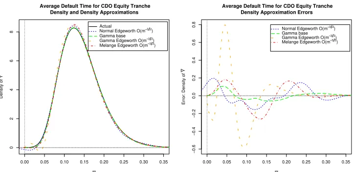
Plots of the approximations (Figure 1) to the average default time density

show overall good performance. The normal Edgeworth expansion is slightly

negative for ¯y < 0.04; the gamma Edgeworth expansion is negative for

0.025 < y <¯ 0.05; and, the gamma base is almost identical to the actual

density. The m´elange (gamma base, normal Edgeworth correction terms)

has almost no negativity and is close to the actual density more often than

the standard normal Edgeworth approximation.

While the gamma Edgeworth approximation has better tail behavior, it

is unfortunately not the best approximation. The mean squared errors

(Ta-ble 2) suggest that the simple gamma base, which still yields economically

meaningful metrics, or the m´elange approach are better approximations.

Normal Edgeworth Gamma Base Gamma Edgeworth M`elange

0.0034 0.0006 0.0306 0.0051

Table 2. Mean-squared errors for density approximations.

Note that the O(ℓ−1/2) gamma base is more accurate than

0.00 0.05 0.10 0.15 0.20 0.25 0.30 0.35 0 2 4 6 8

Average Default Time for CDO Equity Tranche Density and Density Approximations

Y

Density of

Y

Actual

Normal Edgeworth O(m−−3 2) Gamma base Gamma Edgeworth O(m−−3 2) Melange Edgeworth O(m−−3 2)

0.00 0.05 0.10 0.15 0.20 0.25 0.30 0.35

−0.6 −0.4 −0.2 0.0 0.2 0.4 0.6 0.8

Average Default Time for CDO Equity Tranche Density Approximation Errors

Y

Error: Density of

Y

Normal Edgeworth O(m−−3 2) Gamma base Gamma Edgeworth O(m−−3 2) Melange Edgeworth O(m−−3 2)

Figure 1. CDO equity tranche average default time density

approximations (left) and errors (right). The true density is the solid line. Approximations: normal Edgeworth (- -);

gamma base (— —); gamma Edgeworth (–_···); and,

gamma-normal m´elange (–_·). All are O(ℓ−3/2_{) except the O(ℓ}−1/2₎ gamma base.

4.3. Other CDO Tranches with Major Shock. These plots naturally

raise some questions:

1) What do average default time densities look like for other tranches?

2) What if loans ignored risk events with some probabilitypi>0?

3) What ifpi is inversely-proportional to λi? (i.e.What if issuers with

better credit are less likely to face default acceleration?)

For pi = 0 (as above), average default time densities for other tranches

exhibit left-skew which increases with tranche seniority. The A tranche

density, in particular, is sharply left-skewed with a minor mode on the left,

a non-zero plateau in the middle, and a major mode on the right.

If the probability of ignoring a risk event is higher (pi = 0.5,0.8), the A

tranche average default time looks normally distributed while the mezzanine

default time has slightly less right-skew than for pi = 0; but, even a casual

observer would probably doubt normality.

Finally, if the probability of ignoring the shock is proportional to credit

quality, the A and mezzanine tranche average default times appear

normally-distributed. The equity tranche average default time density is right-skewed

(as for pi= 0).

5. Estimating the Approximating Portfolio

We estimate the approximating portfolio in three steps. First, we estimate

the arrival rate for a systematic risk event (e.g. crisis). Next, we estimate

the idiosyncratic default rates and their acceleration during a systematic

risk event. Finally, we use these parameters to simulate loan portfolios from

which we measure cumulants. The cumulants specify the approximating

portfolio.

To estimate the occurence rate for the systematic risk event, the

maximum-likelihood estimator is simply the number of events per unit of time. For

example, if our systematic risk event were a US recession, we could use the

NBER business cycle data to estimateλs. Since the NBER notes an average

cycle length of 55 months, we would estimate λs= 0.218.

To estimate the default acceleration δ during a risk event, we use data

about loans similar to those in our portfolio and which existed when a

sys-tematic risk event occurred at some timets. If we characterize the loan credit

quality for one of those similar loans iasq(i) (e.g. q(i) _{∈ {}good, mediocre,

likelihood function given default timesti:

L(λ, δ_|ts) =

Y

i∈{defaulted},ti<ts

λ_q(i)e−λq(i)ti_·(1−e−λsts₎

| {z }

pre-crisis defaults

×

Y

i∈{defaulted,ti≥ts}

δλ_q(i)e−δλq(i)(ti−ts)_·e−λsts

| {z }

in-crisis defaults

×

Y

i∈{undefaulted,active}

e−δλq(i)(t−ts)_·e−λsts_.

| {z }

possible future defaults

Y

i∈{undefaulted,repaid}

e−δλq(i)(Ti−ts)

·e−λsts_.

| {z }

undefaulted (censored default) (12)

Ideally, the idiosyncratic default ratesλ_q(i)would be the same as those in

the portfolio we are concerned with approximating. However, even if this is

not the case, we can still get a reasonable estimate of δ if we are willing to

assume a constant distress acceleration of default. We then use the estimated

δ to find the approximating portfolio through simulation. This yields the

metrics of interest: the diversity score and the average credit quality.

5.1. Example: 25-loan Subprime Portfolio. As an example of such

inference, we analyze a portfolio of 25 C-credit loans (q(i) = poor).

We are immediately faced with two possible approaches: We could use

risk-neutral default rates for pricing or physical default rates for risk

man-agement (and an appropriate stochastic discount factor for pricing).

To get risk-neutral default rates, we could look at credit default swaps

(CDSs) for the bonds in our portfolio and assume these did not price in

default correlation with risk factors. Similarly, we could find government,

on those bonds to imply a risk-neutral arrival rate for those risks.

Unfor-tunately, the assumption that bond CDSs do not price in the possibility of

correlated defaults is unlikely since CDSs are forward-looking instruments.

Instead, we look at physical default rates. This has the advantage of

cleanly separating the effect of idiosyncratic defaults from risk factors; and,

this is the measure we would want for risk management.

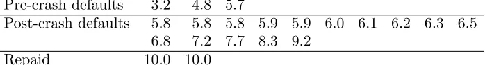
We start by examining (ex post) a portfolio of similar (C-credit) loans

from another recession to find the typical level of default accelerationδ and

idiosyncratic default rateλ_q(i). For a twenty-loan portfolio with the default

times given in Table 3, we would maximize the likelihood equation (12) to

estimate a crisis default-acceleration factor of ˆδ = 3.28 and an idiosyncratic

default rate of ˆλpoor = 0.22.

Pre-crash defaults 3.2 4.8 5.7

Post-crash defaults 5.8 5.8 5.8 5.9 5.9 6.0 6.1 6.2 6.3 6.5

6.8 7.2 7.7 8.3 9.2

Repaid 10.0 10.0

Table 3. Table of loan lifetimes with 3 defaults before a

market crash at 5.8 years; 15 defaults after the crash; and, 2 undefaulted loans which were repaid in full at ten years. The repaid loans are “right censored” since we do not observe default and inference must account for this phenomenon.

Returning to the original portfolio of 25 C-credit loans, we can conduct

an ex ante analysis using the estimated ˆδ and ˆλpoor.11 At time t = 0, we

assume thatλpoor= 0.22 (as estimated).

The interaction between the systematic risk factor and the loans is not

affine, so we cannot easily find a closed-form solution to generate

cumu-lants. Instead, we proceed via simulation as outlined in Algorithm 1. This

simulation is straightforward since we have only one systematic risk factor.

11_{This entails the assumption that the estimated crisis default-acceleration rate ˆδis valid}

Because the inference of ˆλ and ˆℓ assumes we have good estimates of

cumu-lants ˆκ1 and ˆκ2, we average the mean and variance of default times.12 For

10,000 simulations, this gives us the cumulants in Table 4. These

cumu-lants, mean ˆκ1 and variance ˆκ2, jointly determine the iid-loan credit quality

ˆ

λ = ˆκ2

ˆ

κ1 and the diversity score (number of iid loans) ˆℓ = 25df = 25b

ˆ

κ2 1

ˆ

κ2 for

the approximating portfolio.

ˆ

κ1 κˆ2 λˆ dfb ℓˆ 3.170 6.368 0.498 0.634 15.841

Table 4. Table of simulation-averaged cumulants for 10,000

simulations of 25 individual C-credit (subprime) loans with

default acceleration of δ = 3.28 in a recession arriving at

NBER-implied rates. The shared systematic risk factor in-duces default correlation which, in turn, affects the

cumu-lants. The cumulants imply the default intensity ˆλ and

di-versity score ˆℓfor a 25-loan subprime portfolio. Note that the

default-equivalent portfolio is one of just under 16 D-credit loans.

From this analysis, we see that our portfolio of 25 C-credit loans has

de-fault behavior best approximated by a portfolio of just under 16 D-credit

loans. This represents a 37% reduction in diversification strictly due to the

default acceleration from a shared macroeconomic risk factor. Clearly, the

capital adequacy required to hold such a portfolio would be significantly

greater than that required for holding 25 independent C-credit loans

unaf-fected by other risk factors.

6. Conclusion and Future Research

As the above analyses show, the expansions we propose can help analyze

the effects of defaults correlated by default-accelerating risk factors. The

12_{In this section, we switch from working with the average default time in a portfolio}

greatest value from these approximations is the idea of an approximating

portfolio of independent, identical-credit loans and the two

theoretically-based, consistent metrics that approximation yields: ˆℓ, the diversity score

(number of iid loans in the approximating portfolio), and ˆλ, the credit

qual-ity of those loans. While Duffie and Gˆarleanu (2001) estimated the diversqual-ity

score alone, they note that they do not estimate the average loan credit

qual-ity. Thus this paper shows both a different way to estimate the diversity

score and jointly estimates the diverstiy score with the average loan credit

quality.

A further benefit is that many of these approximations perform well at

approximating the average default density. Ideally, we want the distribution

of total default; and, these approximations may be useful to achieving that.

One possibility would be to use the average default time distribution along

with the iid-equivalent loan count. The portfolio would then be modeled as

experiencing total default after all ˆℓiid loans had defaulted.

As for the approximations themselves, the gamma Edgeworth expansion

is mathematically concise and novel. Furthermore, the gamma Edgeworth

expansion, the m´elange, and even the base gamma density all have tail

be-havior that is thicker than standard Edgeworth expansions: tail decay on

the order of e−y instead of e−y2. Furthermore, the gamma and m´elange

expansions add correction terms to better capture the tail risk which Duffie

and Gˆarleanu (2001) raised as an issue with most reduced-form approaches.

While not detectable from the plots, these features are important for

analy-ses involving extreme events: the standard Edgeworth approximations (and

One shortcoming of gamma Edgeworth expansions not shown here is their

poor performance at approximating distributions which are left-skewed.13

An effective way to handle this might be to use the maturity timeT to model

the left-skewed distribution with a y-reversed gamma base or correction

terms originating fromy=T. The reversed gamma densities used would be

of the formγℓ,λ(T−y). A mixture of standard and reversed gamma densities

could be even be used, dictated by the signs of the cumulant differences.

Another area for further work is to study when the implied gamma base

parameter ˆℓis close to violating regularity conditions. In these cases, is may

be fruitful to bias ˆℓupward so the gamma-correction terms may be used.

While standard Edgeworth procedure is to match the first two moments,

this may not be optimal. One could investigate the performance of

Edge-worth expansions where the pseudocumulants are determined by maximum

likelihood or by minimizing some measure of the distance between the

ap-proximate and actual densities. The performance of such maximum-likelihood

“Edgeworth expansions” is surely better than using pseudocumulants;

how-ever, the approximation order is then a model selection question. Such an

approach would probably incorporate higher-order cumulant effects via the

optimization — and thus might be between the Edgeworth and saddlepoint

expansions in both accuracy and spirit.

Appendix A. Multi-Risk Factor-Correlated Default Times

To simulate default times affected by multiple shocks, we first must keep

track of which loans are affected by which shocks. Therefore, we set:

Ai :=_{j_{∈ {}1, . . . , ℓ_}: loan iaffected by risk factorj_}.

(A.1)

13_{Simulations of CDO A tranches suggested that their average default times were}

Algorithm 2. (Multi-Risk Factor-Correlated Default Times)

1) Generate idiosyncratic default times: X˜_{i∈{1,...,ℓ}}indep_∼ Exp(λi).

2) Generate systematic shock times: X˜j∈{ℓ+1,...,ℓ+k}∼Exp(λℓ+j).

3) Sort the systematic shock timesXℓ+1, . . . , Xℓ+kto generate risk-factor

order statistics: X₍₁₎<_{· · ·}< X_(k).

4) Reorder the acceleration coefficients δj similarly to getδ(j).

5) For i= 1 to ℓ, process each loan.

(a) Hold last risk factor shock time: Li = 0.

(b) Forj = 1 to k, examine each risk factor (in time order).

1: If X˜i >X˜(j) and (j)∈ Ai:

Shock (j) affected loan i.

(A) Accelerate default due to risk factor (j) shock:

˜

Xi = ˜Xi/δ(j).

(B) Remember the latest risk shock time:

Li= ˜X(j).

(c) Set risk factor-affected default time: Xi := ˜Xi+Li.

References

Banasik, J.,J. N. Crook, and L. C. Thomas(1999): Not If But When

Will Borrowers Default. Journal of the Operational Research Society

50(12), 1185–1190.

Black, F. and J. C. Cox (1976): Valuing Corporate Securities: Some

Effects of Bond Indenture Provisions. Journal of Finance 31(2), 351–367.

Chambers, J. M. (1967): On Methods of Asymptotic Approximation for

Multivariate Distributions. Biometrika 54(3/4), 367–383.

Collin-Dufresne, P., R. Goldstein, and J. Hugonnier (2004): A

1377–1407.

Cox, D. R. and O. E. Barndorff-Nielsen (1989): Asymptotic

Tech-niques for Use in Statistics. London: Chapman and Hall.

Cox, D. R.and N. Reid (1987): Approximations to Noncentral

Distribu-tions. Canadian Journal of Statistics / Revue Canadienne de Statistique

15(2), 105–114.

Das, S. R., D. Duffie, N. Kapadia, and L. Saita (2007): Common

Failings: How Corporate Defaults Are Correlated. Journal of Finance

62(1), 93–117.

Duffie, D.,A. Eckner,G. Horel, and L. Saita (2009): Frailty

Corre-lated Default. Journal of Finance 64(5), 2089–2123.

Duffie, D.andN. Gˆarleanu(2001): Risk and Valuation of Collateralized

Debt Obligations. Financial Analyst’s Journal 57(1), 41–59.

Edgeworth, F. Y. (1883): On the Method of Ascertaining a Change in

the Value of Gold. Journal of the Statistical Society of London 46(4),

714–718.

Edgeworth, F. Y. (1905): The Law of Error. Transactions of the

Cam-bridge Philosophical Society 20, 35–65,113–141.

Edgeworth, F. Y.(1906): The Generalised Law of Error, or Law of Great

Numbers. Journal of the Royal Statistical Society 69(3), 497–539.

Erlang, A. K. (1909): The Theory of Probabilities and Telephone

Con-versations. Nyt Tidsskrift for Matematik B(20), 33–39.

Feller, W. (1971): An Introduction to Probability Theory and Its

Appli-cations, vol. II. 2nd edn. New York: John Wiley and Sons.

Fender, I.andJ. Kiff(2004): CDO Rating Methodology: Some Thoughts

on Model Risk and its Implications. Working Paper 163, Bank for

Financial Crisis Inquiry Commission (2011): Final Report of the

Na-tional Commission on the Causes of the Financial and Economic Crisis in

the United States. The Financial Crisis Inquiry Report, United States of

America.

Giesecke, K.(2003): A Simple Exponential Model for Dependent Defaults.

Journal of Fixed Income 13(3), 74–83.

Giesecke, K.(2006): Default and Information. Journal of Economic

Dy-namics and Control 30(11), 2281–2303.

Gram, J. P. (1883): ¨Uber die Entwickelung reeler Funktionen in Reihen

mittelstder Methode der kleinsten Quadrate. Journal f¨ur die reine und

angewandte Mathematik 94, 41–73.

Jarrow, R. A., D. Lando, and S. M. Turnbull (1997): A Markov

Model for the Term Structure of Credit Risk Spreads. Review of Financial

Studies 10(2), 481–523.

Jarrow, R. A.andS. M. Turnbull(1995): Pricing Derivatives on

Finan-cial Securities Subject to Credit Risk. Journal of Finance 50(1), 53–85.

Jarrow, R. A. and F. Yu (2001): Counterparty Risk and the Pricing of

Defaultable Securities. Journal of Finance 56(5), 1765–1799.

Leland, H. E. and K. B. Toft (1996): Optimal Capital Structure,

En-dogenous Bankruptcy, and the Term Structure of Credit Spreads. Journal

of Finance 51(3), 987–1019.

Lucas, D.(2001): CDO Handbook. New York: JP Morgan Securities.

Marshall, A. W.and I. Olkin (1967): A Multivariate Exponential

Dis-tribution. Journal of the American Statistical Association 62(317), 30–44.

McCullagh, P.(1987): Tensor Methods in Statistics. London: Chapman

and Hall.

Merton, R.(1974): On the Pricing of Corporate Debt: The Risk Structure

Patnaik, P. B.(1949): The Non-Centralχ2- andF-Distribution and their

Applications. Biometrika 36(1/2), 202–232.

Schorin, C. N.andS. Weinreich(1998): Collateralized Debt Obligation

Handbook. Working paper, Fixed Income Research, Morgan Stanley.

Thiele, T. N. (1871): En mathematisk Formel for Dødeligheden, prøvet

paa en af Livsforsikringanstalten af 1871 benyttet Erfaringrække.

Copen-hagen: C. A. Reitzel.

Thiele, T. N. (1872): On a Mathematical Formula to Express the Rate

of Mortality Throughout the Whole of Life. Journal of the Institute of

Actuaries 16, 313–329. Translated by T. B. Sprague.

Tung, J., A. Metz, and N. Weill (2011): Default and Loss Rates of

Structured Finance Securities: 1993–2010. Special comment, Moody’s

Investors Service.

Zhou, C. (2001): An Analysis of Default Correlations and Multiple