Reduce computation in profile empirical likelihood method

Reduce computation in profile empirical

likelihood method

Li, Minqiang and Peng, Liang and Qi, Yongcheng

2011

Online at

https://mpra.ub.uni-muenchen.de/33744/

LIKELIHOOD METHOD∗

By Minqiang Li, Liang Peng, and

Yongcheng Qi

Bloomberg LP, Georgia Institute of Technology and University of Minnesota Duluth

Since its introduction by Owen in [29, 30], the empirical

likeli-hood method has been extensively investigated and widely used to

construct confidence regions and to test hypotheses in the literature.

For a large class of statistics that can be obtained via solving

esti-mating equations, the empirical likelihood function can be formulated

from these estimating equations as proposed by [35]. If only a small

part of parameters is of interest, a profile empirical likelihood method

has to be employed to construct confidence regions, which could be

computationally costly. In this paper we propose a jackknife

empiri-cal likelihood method to overcome this computational burden. This

proposed method is easy to implement and works well in practice.

1. Introduction. Empirical likelihood method was introduced by Owen ([29,30] ) to construct confidence regions for the mean of a random vector.

Like the bootstrap and jackknife methods, the empirical likelihood method is a nonparametric one. Without assuming a family of distributions for the

∗_{Peng’s research was supported by NSA Grant H98230-10-1-0170 and NSF Grant}

DMS1005336. Qi’s research was supported by NSA Grant H98230-10-1-0161 and NSF Grant DMS1005345.

AMS 2000 subject classifications:Primary 62E20; secondary 62F12

Keywords and phrases:profile empirical likelihood, estimating equation, Jackknife

data, the empirical likelihood ratio statistics can be defined to share similar properties as the likelihood ratio for parametric distributions. For instance,

the empirical likelihood method produces confidence regions whose shape and orientation are determined entirely by the data. In comparison with

the normal approximation method and the bootstrap method for

construct-ing confidence intervals, the empirical likelihood method does not require a pivotal quantity, and it has better small sample performance (see [15]).

As an effective way for interval estimation and goodness-of-fit test, the empirical likelihood method has been extended and applied in many different

fields such as regression models ([11]), quantile estimation ([9]), additive risk models ([22]), two-sample problems ([36], [19], [3], [43]), time series models

([16], [14], [8], [28], [27], [4], [5]), heavy-tailed models ([21], [32], [33, 34]), high dimensional data ([10]) and copulas ([6]).

A common feature in employing the empirical likelihood method is to work with linear constraints such as linear functionals, and a powerful way in

for-mulating the empirical likelihood ratio statistic is via estimating equations as in [35]. When the constraints involve nonlinear equations, an important

trick is to transform these nonlinear constraints to some linear constraints by introducing some link variables. After this transformation, a profile

empiri-cal likelihood method is employed. For example, if one wants to construct an empirical likelihood confidence interval for the varianceθ=E_{X₋EX_}2_,

one can introduce a link variableβ =E(X) and then formulate the empir-ical likelihood by using equations E(X) = β and E(X2_{) = θ+β}2_{. Some}

more computational burden to the empirical likelihood method. Another computational difficulty arises when the profile empirical likelihood method

involves a large number of nuisance parameters.

SupposeX1,· · · , Xn are independent random vectors with common

dis-tribution function F and there is a q-dimensional parameter θ associated

withF. LetyT denote the transpose of the vectory and

G(x;θ) = (g1(x;θ),· · ·, gs(x;θ))T

denote s(_≥ q) functionally independent functions, which connect F and

θ through the equations EG(X1;θ) = 0. Write θ = (αT, βT)T, where α

and β are q1-dimensional and q2-dimensional parameters, respectively, and

q1+q2 =q. In order to construct confidence regions forα, [35] proposed to

use the following profile empirical likelihood ratio

(1.1) l(α) = 2lE((αT,βˆT(α))T)−2lE(˜θ),

where lE(θ) = Pni=1log{1 +tT(θ)G(Xi;θ)}, t =t(θ) is the solution of the

following equation

(1.2) 0 = 1

n

n

X

i=1

G(Xi;θ)

1 +tT_G(X i;θ)

,

˜

θ = (˜αT,β˜T)T minimizes lE(θ) with respect to θ, and ˆβ(α) minimizes

lE((αT, βT)T) with respect to β for fixed α. It has been shown that l(α0)

converges in distribution toχ2_q1 under some regularity conditions, whereα0

denotes the true value ofα. For the second order properties of the empirical

likelihood method based on estimating equations, we refer to [7].

The computational complexity in using the profile empirical likelihood

method comes from computinglE((αT,βˆT(α))T). When the nuisance

ofβ so that the computation is reduced significantly. In order to avoid com-putinglE((αT,βˆT(α))T), one may choose to replace ˆβT(α) by some other

dif-ferent estimator, for example, solvingq2 equations ofn−1Pni=1G(Xi;θ) = 0.

Although this reduces computation especially when one can find an explicit

estimator of β in terms of the sample andα, Wilks’ theorem doesn’t hold,

that is,l(α0) does not converge in distribution toχ2q1. Instead,l(α0) generally

converges in distribution to a weighted sum of independent chi-square

ran-dom variables; see [17]. Since the weights in the limit have to be estimated, this empirical likelihood method does not preserve the important properties

of the standard empirical likelihood method: self-studentization, automati-cally determined shape of confidence region and Bartlett correction.

There-fore, it is of importance to develop an empirical likelihood method which has a chi-square limit and is computationally efficient than the profile

empiri-cal likelihood method especially when the number of nuisance parameters is large. Moreover, when some estimating equations involve U-statistics, the

profile empirical likelihood method is extremely complicated.

Motivated by the recent study on using jackknife empirical likelihood

method to deal with nonlinear constraints in U-statistics ([18]), we propose a jackknife empirical likelihood method to construct confidence regions for

the interesting parameter α with the nuisance parameter β being simply replaced by some estimator. The jackknife empirical likelihood ratio

statis-tic is obtained by applying the standard empirical likelihood method to the jackknife pseudo sample. The jackknife method was originally used to

likelihood method allows us to compute the nuisance parameters simply through a subset of estimating equations and yet still retains the attractive

chi-square limiting distribution for the empirical likelihood ratio.

We organize this paper as follows. In Section 2, the new methodology

and main results are given. Section3presents a simulation study. Section 4

presents two case studies of financial applications. All proofs are given in Section5.

2. Methodology and main results. As in the introduction, letG(x;θ) = (g1(x;θ),· · ·, gs(x;θ))T denote s(≥ q) functionally independent functions

with EG(X1;θ0) = 0, where θ0 = (αT0, β0T)T denotes the true value of

θ = (αT, βT)T, and α and β are q1-dimensional and q2-dimensional

pa-rameters, respectively. Note that only the parameter α is of interest under consideration. To remove the nuisance parameterβ, we propose to first

esti-mate it from someq2 estimating equations, and then work with the

remain-ing s₋q2 equations, where β is replaced by the obtained estimator. The

details are as follows. Define

Ga(x;α, β) =¡g1(x;α, β),· · ·, gs−q2(x;α, β)

¢T

and

Gb(x;α, β) =¡gs−q2+1(x;α, β),· · · , gs(x;α, β)

¢T .

Without loss of generality, we solve the lastq2equations ofn−1Pni=1G(Xi;θ)

to get an estimator forβ. That is, ˜β(α;X) is the solution to

(2.1) 1

n

n

X

i=1

with respect to β for each fixed α, where X = (X1,· · ·, Xn)T. Obviously,

the best choice of theq2 equations is to have explicit formula for ˜β(α;X), if

possible. Set

Tn(α) =

1 n

n

X

i=1

Ga(Xi;α,β(α,˜ X))

and let ˜β(α;X₋i) denote the solution to the equations

(2.2) 1

n₋1

n

X

j=1,j6=i

Gb(Xj;α, β) = 0

with respect toβfor each fixedα, whereX₋i= (X1,· · ·, Xi−1, Xi+1,· · ·, Xn)T.

Similarly, define

Tn,−i(α) = 1

n₋1

n

X

j=1,j6=i

Ga(Xj;α,β(α;˜ X−i)).

Then the jackknife pseudo sample is defined as

Yi(α) = (Yi,1(α),· · ·, Yi,s−q2(α))

T _=nT

n(α)−(n−1)Tn,−i(α) for i= 1,· · · , n.

As in [42], one expects thatY′

isare approximately independent. This

mo-tivates us to apply the standard empirical likelihood method to the jackknife sampleY1(α),· · ·, Yn(α) for constructing empirical likelihood confidence

re-gions forα. Hence we define the jackknife empirical likelihood function as

LJ(α) = supnΠn_i=1(npi) : n

X

i=1

pi= 1, n

X

i=1

piYi(α) = 0, p1≥0,· · · , pn≥0

o .

It follows from the Lagrange multiplier technique that the above maximiza-tion is achieved atpi=n−1{1 +λTYi(α)}−1 and the log empirical likelihood

ratioℓJ(α) =₋logLJ(α) is given by

(2.3) ℓJ(α) =

n

X

i=1

whereλ=λ(α) satisfies

1 n

n

X

i=1

Yi(α)

1 +λT_Y i(α)

= 0. (2.4)

Before we present our main results, we first list the assumptions we need. For this purpose, denote _∂x∂y = (∂yi

∂xj)1≤i≤m,1≤j≤n for y = (y1,· · · , ym)

T _and

x= (x1,· · · , xn)T, and define

ˆ

α= arg minℓJ(α), Σ =¡

E_{gk(X1;α0, β0)gl(X1;α0, β0)}¢_1≤k,l≤s= (σk,l)1≤k,l≤s,

Σ1 =E{

∂

∂βGb(X1;α0, β0)}, Σ2=E{ ∂

∂αGb(X1;α0, β0)},

Σ3 =E{

∂

∂αGa(X1;α0, β0)} −E{ ∂

∂βGa(X1;α0, β0)}Σ

−1

1 Σ2

and Σ∗ _{= (σ}∗

k,l)1≤k,l≤s−q2,where

σ∗

k,l =σk,l−E{_∂β∂ gk(X1;α0, β0)}Σ−11(σs−q2+1,l,· · ·, σs,l)

T

−E_{∂β∂ gl(X1;α0, β0)}Σ−11(σs−q2+1,k,· · · , σs,k)

T

+E_{∂β∂ gk(X1;α0, β0)}Σ1−1(σij)s−q2+1≤i,j≤sΣ−

1

1 E{∂β∂Tgl(X1;α0, β0)}.

Some regularity conditions are as follows:

• A1) There is a neighborhood of α0 and β0, say Ωα0 ×Ωβ0, such that

Gb(x;α, β) are continuous function of α ∈ Ωα0 and β ∈ Ωβ0 for all

x, and sup_α∈Ωα

0,β∈Ωβ0||Gb(x;α, β)||

3 _{≤ K(x) for some function K}

satisfying thatEK(X1)<∞;

• A2) For each α _∈ Ωα0, there is a function β(α) ∈ Ωβ0 such that

EGb(X1;α, β(α)) = 0;

• A3) _||∂β∂ Gb(x;α, β)||3, || ∂

2

∂βT_∂βgl(x;α, β)||3 and | ∂

3

∂βi∂βj∂βmgl(x;α, β)|

for l = s₋q2 + 1,· · ·, s, i, j, m = 1,· · · , q2 are bounded by K(x)

• A4)β(α) defined in A2) has continuous first derivatives;

• A5)_||∂α∂ Gb(x;α, β)||3and| ∂

3

∂αi∂βj∂βmgl(x;α, β)|forl=s−q2+1,· · ·, s,

i = 1,_{· · ·}, q1, j, m = 1,· · ·, q2 are bounded by K(x) uniformly in

α_∈Ωα0 andβ ∈Ωβ0;

• A6) Assume Σ1 is invertible, Σ∗ is positive definite and Σ3 has rank

q1;

• A7)_||∂β∂ Ga(x;α, β)||,||Ga(x;α, β)||3,| ∂

3

∂αk∂βj∂βmgl(x;α, β)|and

|∂βi∂β∂3j∂βmgl(x;α, β)| for i, j, m = 1,· · ·, q2, k = 1,· · ·, q1 and l =

1,_{· · ·} , s₋q2 are bounded byK(x) uniformly inα∈Ωα0 andβ ∈Ωβ0.

The following two propositions show the existence and some properties of ˜

β(α;X), ˜β(α0;X−i) and ˆα.

Proposition 1. i) Under conditions A1) and A2), with probability one, there exist solutions ˜β(α;X)_∈Ωβ0 and ˜β(α;X−i)∈Ωβ0 to (2.1) and (2.2),

respectively, such that

(2.5) β(α;˜ X)₋β(α) =o(1) and max

1≤i≤n||

˜

β(α;X₋i)−β(α)||=o(1)

almost surely for eachα_∈Ωα0.

ii) Under conditions A1)–A3), we have

(2.6) β(α˜ 0;X)−β0+ Σ−11

1 n

n

X

i=1

Gb(Xi;α0, β0) =Op(n−1),

(2.7) max

1≤i≤n||

˜

β(α0;X−i)−β0+Σ−11

1 n₋1

n

X

j=1,j6=i

Gb(Xj;α0, β0)||=Op(n−1),

(2.8) max

1≤i≤n||

˜

where

Σn1 =

1 n n X j=1 ∂

∂βGb(Xj;α0,β(α˜ 0;X)), Dn(i) = (Dn,s−q2+1(i),· · ·, Dn,s(i))

T

and

Dn,l(i)

= 1₂n−1_GT

b(Xi;α0, β0)Σ−11E{ ∂

2

∂βT_∂βgl(X1;α0, β0)}Σ₁−1n−1Gb(Xi;α0, β0)

+n−1gl(Xi;α0, β0)−n−1{_∂β∂ gl(Xi;α0, β0)}Σ−11n−11

Pn

j=1Gb(Xj;α0, β0)

+n−1_{ ∂

∂βgl(Xi;α0, β0)}Σ1−1n−11Gb(Xi;α0, β0).

iii) Under conditions A1)-A5), we have

(2.9)     

max1≤i≤n||_∂α∂ β(α˜ 0;X−i) + Σ−11Σ2||=Op(n−1/2),

||∂α∂ β(α˜ 0;X) + Σ− 1

1 Σ2||=Op(n−1/2),

and

(2.10) max

1≤i≤n||

∂

∂αβ(α˜ 0;X)− ∂

∂αβ(α˜ 0;X−i) + Σ

−1

1 Ai||=op(n−1),

whereAi = (as−q2+1(i),· · · , as(i))

T _and

aT

l (i) =−n1GTb(Xi;α0, β0)Σ−11E{ ∂

2

∂βT_∂αgl(X1;α0, β0)}+_n1_∂α∂ gl(Xi;α0, β0)

+_n1GT_b(Xi;α0, β0)Σ−11E{ ∂

2

∂βT_∂βgl(X1;α0, β0)}Σ−

1 1 Σ2 −n1∂β∂ gl(Xi;α0, β0)Σ−11Σ2.

Proposition 2. Under A1)–A7), with probability tending to one, ℓJ(α) attains its minimum value at some point ˆα in the interior of the ball _||α₋ α0|| ≤n−1/3, and ˆα and ˆλ=λ(ˆα) satisfy

Q1n(ˆα,λ) = 0 andˆ Q2n(ˆα,λ) = 0,ˆ

where

Q1n(α, λ) =

1 n

n

X

i=1

Yi(α)

and

Q2n(α, λ) =

1 n

n

X

i=1

1 1 +λT_Y

i(α){

∂

∂αYi(α)}

T_λ.

Next we show that Wilks’ theorem holds for the proposed jackknife em-pirical likelihood method.

Theorem 1. Under conditions A1)–A7), we have LR(α0) := 2ℓJ(α0) −

2ℓJ(ˆα) converges in distribution toχ2_q1, where ˆα, ˜β(α;X) and ˜β(α;X−i) are

given in Propositions 1 and 2.

Based on Theorem 1, an asymptotically accurate 100γ% confidence region

forα is given by

Iγ={α:LR(α)≤χ2q1(γ)},

whereχ2

q1(γ) is theγquantile of aχ

2_{distribution withq}

1degrees of freedom.

Remark 1.When s=q, we have ℓJ_{(ˆα) = 0. Moreover, when ˜β(α;X) has}

an explicit formula in terms of the sampleXand α, the computation of the proposed jackknife empirical likelihood method is only slightly heavier than

the standard empirical likelihood method. Indeed, the software R package for the empirical likelihood method can be employed as in our simulation

study.

Remark 2.If one is interested in a part ofα= ( ˜αT

1,α˜T2)T, say ˜α1, then we

can show that 2 minα˜2ℓ

J_(α)−2ℓJ_{(ˆα) converges in distribution to a chi-square}

limit with the degrees of freedom being the length of ˜α1. This method may

be called jackknife profile empirical likelihood method, which is appealing

when a part of nuisance parameters can be solved explicitly.

conditions involving the partial derivatives of Gb with respect to α can be

removed.

3. Simulation study. Suppose the random vector (X, Y) has marginal distribution functions F1, F2 and copula C(x, y) = P(F1(X) ≤ x, F2(Y) ≤

y). In fitting a parametric family to the copula, a useful quantity is the

Spearman’s rho defined asρs= 12E{F1(X)F2(Y)} −3. For example, if one

employs the Gaussian copula

C(u, v;θ) =

Z Φ−(u)

−∞

Z Φ−(v)

−∞

1

2π√1₋θ2 exp{−

s2₋2θst+t2 2(1₋θ2₎ }dsdt,

or the t copula

C(u, v;θ) = Z t−4(u)

−∞

Z t−4(v)

−∞

1

2π√1₋θ2{1 +

s2₋2θst+t2 4(1₋θ2₎ }−

3_dsdt,

whereθ_∈[₋1,1] and Φ−_andt−

ν denote the inverse function of the standard

normal distribution function andtdistribution function with degrees of

free-dom ν, respectively, then ρs = 6π−1arcsin(θ/2). Hence, Spearman’s rho is

of importance in fitting a parametric copula. Here, we consider constructing

a confidence interval for the Spearman’s rho by fitting either the Gaussian copula or thet copula and modeling marginals by either a normal

distribu-tion or a t distribution. In this case, a profile empirical likelihood method can be employed to construct a confidence interval forρs by considering the

following estimating equations

      

     

ρs= 12E{F1(X;µ1, σ1)F2(Y;µ2, σ2)} −3

0 =EX₋µ1 =EY −µ2

0 =EX2_−µ2

whenF1 andF2 have normal distributionsN(µ1, σ21) andN(µ2, σ22),

respec-tively, and

  

 

ρs= 12E{F1(X;ν1)F2(Y;ν2)} −3

0 =EX2₋ν1/(ν1−2) =EY2−ν2/(ν2−2)

when F1 and F2 have distributions tν1 and tν2, respectively. On the other

hand, the proposed jackknife empirical likelihood method can be employed

to the above estimating equations as well.

First we draw 10,000 random samples with sample size n = 100 and

300 from the Gaussian copula and t copula by using the package ’copula’ in R and transform the marginals to have either normal distributions or

t distributions. For computing the coverage probabilities of the proposed

jackknife empirical likelihood method, we employ the package ‘emplik’ in the software R. For computing the coverage probabilities of the profile empirical

likelihood method, we use the package ‘emplik’ to obtain the likelihood ratio as a function of nuisance parameters and then use the package ‘nlm’ to find

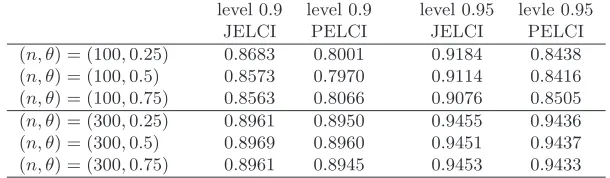
the minimum. These coverage probabilities are reported in Tables 1–4. From Tables 1–4, we observe that i) the proposed jackknife empirical likelihood

method performs much better than the profile empirical likelihood method whenn= 100 and marginal distributions follow fromtdistributions; and ii)

both methods perform well when n= 300 although the jackknife empirical likelihood method is slightly better.

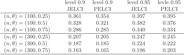
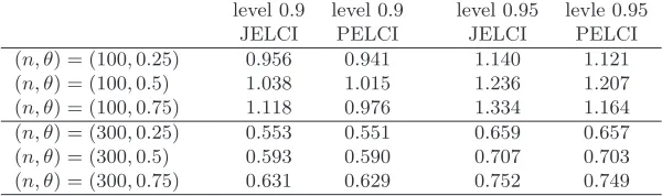
Second, we calculate the average interval lengths for both methods by drawing 1,000 random samples from the above models. Tables 5-8 show that

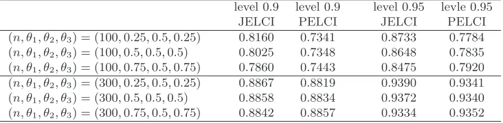
Third, we draw 10,000 random samples from a 3-dimensional normal cop-ula and t copcop-ula with marginal distributions t7, t8, t9 and θ= (θ1, θ2, θ2)T.

Then we apply the proposed jackknife empirical likelihood method and the profile empirical likelihood method to construct confidence regions for the

three Spearman’s rho. Coverage probabilities are reported in Tables 9 and

10, which show that the proposed jackknife empirical likelihood method performs better than the profile empirical likelihood.

In conclusion, the proposed jackknife empirical likelihood method pro-vides good coverage accuracy and the computation is much simpler than

the profile empirical likelihood method. Moreover, the package “emplik” in the software R is ready to use for the proposed method.

4. Case studies.

4.1. Testing the drift parameter in the variance gamma model. The class of variance gamma (VG) distributions was introduced by [25] as an alterna-tive model for stock returns beyond the usual normal distribution

assump-tion. It has so far been used extensively by financial economists especially in pricing financial derivatives, see [24] and [23] for applications, and [38] for

a historical account of the development.

The VG processZt is a time-changed L´evy process where the

subordina-tor is a Gamma process. It is parameterized by three parameters: the drift parameterµ, the volatility parameter σ, and the subordinator variance

pa-rameterν. More specifically, let St be a gamma process subordinator with

a unit mean rate and a variance rateν whereν >0. Let Wt be a standard

That is, the calendar time t is now replaced with the time change St. Let

X _≡ Zt+δ−Zt be the increment of Zt with interval δ. The characteristic

function ofX is EeiuX =eΨ(u)δ, where the characteristic exponent Ψ(u) is given by Ψ(u) =_−ν1log_{1 +u2σ₂2ν ₋iµνu_}.

Given a sampleX of incrementsX with sample size n, we are interested

in the hypothesis H0 : µ = 0. This amounts to asking whether it is

suffi-cient to model the data in interest using a martingale process. For example,

it is interesting to know whether one needs to introduce a drift parameter for the log change of US/Japan exchange rate process or not. The

param-eter of interest is thus µ, and the two nuisance parameters are (σ, ν). To employ the jackknife empirical likelihood estimation method in this paper,

we need the estimating equations. One approach would be to just use the mean equation alone. However, this ignores all higher moments which are

the very reason why financial economists use variance gamma process as an alternative to Brownian motion with drift. Therefore, below we use a

differ-ent approach based on higher-order momdiffer-ents. The lowest-order momdiffer-ents or central moments would seem to be natural choices. However, the odd

mo-ments or central momo-ments are all proportional toµand thus all zero under the nullH0 : µ= 0. Thus we use only the even moments with orders 2, 4

and 6.

By differentiating the characteristic function of the VG process increment,

the raw even moments mj(µ, ν, σ) := EXj can be computed easily and

estimating equations are obtained by equating the empirical moments to

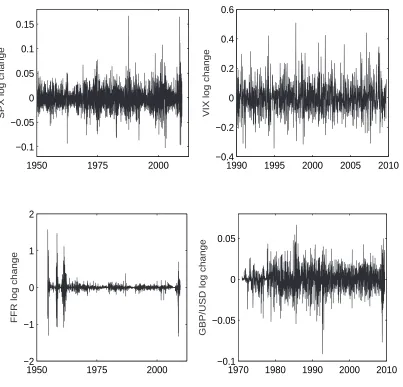
We use four different financial time series, namely, the S&P 500 index (SPX), the CBOE volatility index (VIX), the effective federal funds rate

(FFR), and the exchange rate between the British Pound and US Dollar (GBP/USD). These four time series are very important in four distinctive

large financial sectors, that is, the equity market, the financial derivative

market, the fixed-income market, and the foreign exchange market. The sample periods are January 1950 to October 2009 for the SPX, January

1990 to October 2009 for the VIX, July 1954 to September 2009 for the FFR, and January 1971 to July 2009 for the GBP/USD.

Figure 1plots these four time series on the same graph. The subplot for the SPX shows a few significant events, including the amazing run of the

SPX before year 1987, the market crash in 1987, the internet boom in late 90s, the IT bubble burst in 2001, and most recently the subprime mortgage

crisis. From the second subplot, we see that the VIX has been largely stable, except for the abrupt surge during the recent market turmoil. The FFR has

had quite a few surges, especially during the hyper-inflation period in the late 70s and early 80s, and has recently reached unprecedented low levels

due to the Fed’s effort to boost the economy. The most noticeable feature on the GBP/USD subplot is the free fall and fast appreciation of the British

Pound before and after the Plaza Accord in 1985. The recent global financial crisis has also weakened the British Pound due to the flight to quality by

international investors.

Our samples are the weekly log change processes of the above four

dis-tribution assumption, see for example [2] or [20]. [26] traces awareness of this non-normality as far back as year 1915. This nonnormality is especially

true for the times series of the log change of the effective federal funds rate, where we see a huge kurtosis.

Table11reports the test statisticLR(0) for the log changes of the four

fi-nancial time series considered. The statistic is asymptoticallyχ2₁distributed, and the asymptoticp-values are reported. The skewness and kurtosis for each

time series are also included in the table, as well as the result of a naive t-test. As we would expect, the statisticLR(0) strongly rejects H0 : µ = 0

for the log changes of the S&P 500 index with a p-value of only 0.0002. However, the statistic cannot rejectH0 : µ= 0 for the log changes of the

CBOE volatility index, and the exchange rate between British Pound and US Dollar. These are the same conclusions one gets from the naivet-test

as-suming that the sample is drawn from a normal distribution with unknown variance. However, the test on the log changes of FFR is interesting. A naive

t-test suggests that µ = 0, while the test statistic LR(0) rejects µ = 0 at more than 99% level. This apparent discrepancy might be explained by the

fact that we have used higher-order moments in the estimating equations and that the empirical distribution of log changes of FFR is very different

from the normal distribution with a very large kurtosis. It also highlights the advantage of using empirical likelihood estimation over the naivet-test

which assumes a normal distribution.

4.2. Testing whether a normal tempered stable process is normal inverse

of models is obtained by time changing an independent Brownian motion with drift by a tempered stable subordinator St. The L´evy measure of St

with indexA and parameterν is given by

ρS(x) =

1 Γ(1₋A)

µ₁ −A

ν

¶1−A_e−(1−A)x/ν

xA+1 1x>0,

where ν > 0 and 0 _≤ A < 1 are two constants. The increment X of the time-changed processYtagain has a closed-form characteristic function with

characteristic exponent as follows

Ψ(u) = 1−A νA

 

 1₋

Ã

1 +ν(u

2_σ2_/2−iµu

1₋A

!A 

 .

Two important special cases are the VG process (where A = 0) and the

normal inverse Gaussian process (whereA= 1/2). See [1] and [37] for early studies on the normal inverse Gaussian process.

We are now interested in the null hypothesis H0 : A = 1/2, that is,

whether the data implies a normal inverse Gaussian process. Thus, the

pa-rameter of interest is A and the nuisance parameters are now (µ, ν, σ). To employ the jackknife empirical likelihood estimation method, we construct

estimating equations from the raw momentsmj(A, µ, ν, σ) :=EXj. It turns

out that ifµ= 0 in the normal tempered stable process, then the lowest four

moments are not functions of A. Also, if µ= 0, then all odd moments are zero. Thus, to reliably estimateA using moments whenµis small, we have

to include a momentmj withj≥6. We choose to use the momentsm1,m2,

m4 and m6 which can be calculated straightforwardly. Then the jackknife

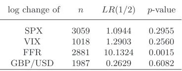
We apply the above procedure to the same four time series as before. The results are shown in Table12. As we see, the test statistic LR(1/2) cannot

reject H0 : A = 1/2 for the log changes of the S&P 500 index, the CBOE

VIX index, and the exchange rate between the British Pound and US Dollar.

However, it strongly rejects A = 1/2 for the log change time series of the

effective federal funds rate.

5. Proofs. Proof of Proposition 1.Since condition A1) implies that

(5.1) max

1≤i≤n_βsup_∈Ωβ

0

1

n₋1||Gb(Xi;α, β)||=o(n

−1/2₎

almost surely for eachα_∈Ωα0, we have

1 n−1

Pn

j=1,j6=iGb(Xj;α, β) = _n−1₁Pnj=1Gb(Xj;α, β)−_n−1₁Gb(Xi;α, β) → EGb(X1;α, β)

almost surely and uniformly in 1_≤i_≤n for α_∈ Ωα0 and β ∈Ωβ0. Hence

Part i) follows from the above equation and Theorem B in Section 7.2.1 of [39].

It follows from Taylor’s expansion that (5.2)

0 = _n−1₁Pn

j=1,j6=iGb(Xj;α0,β(α˜ 0;X−i))

= _n−1₁Pn

j=1,j6=iGb(Xj;α0, β0)

+_n−1₁Pn

j=1,j6=i{∂β∂ Gb(Xj;α0, γiβ0+ (1−γi) ˜β(α0;X−i))}{β(α˜ 0;X−i)−β0},

whereγi ∈[0,1] for eachi= 1,· · ·, n. Since A1) and (2.5) imply that

(5.3)

max

1≤i≤n

1

n₋1||Gb(Xi;α0, γiβ0+(1−γi) ˜β(α0;X−i))||=o(n

we have (5.4)

max

1≤i≤n||

1 n₋1

n

X

j=1,j6=i

∂

∂βGb(Xj;α0, γiβ0+ (1−γi) ˜β(α0;X−i))−Σ1||=op(1).

Hence (2.7) follows from (5.2) and (5.4). Similarly we can prove (2.6). By (2.6), (2.7) and (5.3), we have

(5.5)

  

 

max1≤i≤n||β(α˜ 0;X)−β(α˜ 0;X−i)||=op(n−1/2)

max1≤i≤n||β(α˜ 0;X−i)−β0||=Op(n−1/2).

It follows from (5.5) and Taylor’s expansion that

0 = _n1_{Pn

j=1Gb(Xj;α0,β(α˜ 0;X))−Pnj=1,j6=iGb(Xj;α0,β(α˜ 0;X−i))}

= _n1 Pn

j=1{Gb(Xj;α0,β(α˜ 0;X))−Gb(Xj;α0,β(α˜ 0;X−i))}

+n−1_G

b(Xi;α0,β(α˜ 0;X−i))

= Σ1{β(α˜ 0;X)−β(α˜ 0;X−i)}+op(n−1)

+n−1_G

b(Xi;α0, β0) +op(n−1)

uniformly in 1_≤i_≤n, which implies that

(5.6) max

1≤i≤n||

˜

β(α0;X)−β˜(α0;X−i) + Σ−11

1

nGb(Xi;α0, β0)||=op(n

−1_).

Note that A3) implies that

(5.7) max

1≤i≤n_α∈Ωαsup

0,β∈Ωβ0

||n−1 ∂

2

∂βT_∂βgl(Xi;α, β)||=o(n− 1/2₎

Using (2.7), (5.5)–(5.7) and Taylor’s expansion, we have

0 = 1_n{Pn

j=1gl(Xj;α0,β(α˜ 0;X))−Pnj=1,j6=igl(Xj;α0,β(α˜ 0;X−i))}

= 1_nPn

j=1{gl(Xj;α0,β(α˜ 0;X))−gl(Xj;α0,β(α˜ 0;X−i))}

+n−1_g

l(Xi;α0,β(α˜ 0;X−i))

= 1_nPn

j=1{∂β∂ gl(Xj;α0,β˜(α0;X))}{β(α˜ 0;X)−β(α˜ 0;X−i)}

+_2n1 Pn

j=1{β(α˜ 0;X)−β(α˜ 0;X−i)}T{ ∂

2

∂βT_∂βgl(Xj;α0,β(α˜ 0;X))}

{β(α˜ 0;X)−β(α˜ 0;X−i)}+n−1gl(Xi;α0, β0)

+n−1_{ ∂

∂βgl(Xi;α0, β0)}{β(α˜ 0;X−i)−β0}+op(n−3/2)

= 1_nPn

j=1{∂β∂ gl(Xj;α0,β˜(α0;X))}{β(α˜ 0;X)−β(α˜ 0;X−i)}

+_2n1 _{n1GT

b(Xi;α0, β0)Σ−11}{Pnj=1 ∂

2

∂βT_∂βgl(Xj;α0,β(α˜ 0;X))}

{Σ−₁11_nGb(Xi;α0, β0)}+n−1gl(Xi;α0, β0)

−n−1_{∂β∂ gl(Xi;α0, β0)}Σ−11n−11

Pn

j=1,j6=iGb(Xj;α0, β0)

+op(n−3/2)

=_{1_nPn

j=1∂β∂ gl(Xj;α0,β(α˜ 0;X))}{β(α˜ 0;X)−β(α˜ 0;X−i)}

+1_2{1_nGT_b(Xi;α0, β0)Σ−11}{E ∂

2

∂βT_∂βgl(X1;α0, β0)}

{Σ−₁11_nGb(Xi;α0, β0)}+n−1gl(Xi;α0, β0) −n−1_{ ∂

∂βgl(Xi;α0, β0)}Σ−11n−11

Pn

j=1Gb(Xj;α0, β0)

+n−1_{∂β∂ gl(Xi;α0, β0)}Σ1−1n−11Gb(Xi;α0, β0) +op(n−3/2)

uniformly in 1_≤i_≤nforl=s₋q2+ 1,· · ·, s, which imply (2.8).

Since 0 = _n−1₁Pn

j=1,j6=iGb(Xj;α,β(α;˜ X−i)), we have

0 = _n−1₁Pn

j=1,j6=i ∂α∂ Gb(Xj;α,β(α;˜ X−i))

+_n−1₁Pn

j=1,j6=i{∂β∂ Gb(Xj;α,β(α;˜ X−i))}_∂α∂ β(α;˜ X−i).

Note that A5) implies that

max

1≤i≤n

1 n₋1||

∂

∂αGb(Xi;α0,β(α˜ 0;X−i))||=o(n

almost surely. Hence

∂

∂αβ(α˜ 0;X−i) =−Σ

−1

1 Σ2+Op(n−1/2)

uniformly in 1_≤i_≤n. Similarly, we have

∂

∂αβ(α˜ 0;X) =−Σ

−1

1 Σ2+Op(n−1/2),

i.e., (2.9) holds.

It follows from (5.5), (5.6), A3) and A5) that

1 n

Pn

j=1{∂α∂ gl(Xj;α0,β(α˜ 0;X))−∂α∂ gl(Xj;α0,β˜(α0;X−i))}

= 1_nPn

j=1{β(α˜ 0;X)−β(α˜ 0;X−i)} ∂

2

∂βT_∂αgl(Xj;α0, β0) +op(n−1)

= _−n1GT_b(Xi;α0, β0)Σ−11E{ ∂

2

∂βT_∂αgl(X1;α0, β0)}+op(n−1)

and

1 n

Pn

j=1{∂β∂ gl(Xj;α0,β(α˜ 0;X))−∂β∂ gl(Xj;α0,β(α˜ 0;X−i))}

= _n1Pn

j=1{β(α˜ 0;X)−β(α˜ 0;X−i)} ∂

2

∂βT_∂βgl(Xj;α0, β0) +op(n−1)

= ₋1_nGT_b(Xi;α0, β0)Σ−11E{ ∂

2

uniformly in 1_≤i_≤nforl=s₋q2+ 1,· · ·, s. Hence

0 = _n1_{Pn

j=1∂α∂ gl(Xj;α0,β(α˜ 0;X))−

Pn

j=1,j6=i ∂α∂ gl(Xj;α0,β(α˜ 0;X−i))}

+_n1_{Pn

j=1

¡ ∂

∂βgl(Xj;α0,β(α˜ 0;X))

¢ ∂

∂αβ(α˜ 0;X) −Pn

j=1,j6=i

¡_∂

∂βgl(Xj;α0,β(α˜ 0;X−i))

¢ _∂

∂αβ(α˜ 0;X−i)}

= _n1 Pn

j=1{∂α∂ gl(Xj;α0,β(α˜ 0;X))−∂α∂ gl(Xj;α0,β(α˜ 0;X−i))}

+_n1_∂α∂ gl(Xi;α0,β˜(α0;X−i))

+_n1Pn

j=1{∂β∂ gl(Xj;α0,β(α˜ 0;X))−∂β∂ gl(Xj;α0,β(α˜ 0;X−i))}_∂α∂ β(α˜ 0;X)

+_n1Pn

j=1{∂β∂ gl(Xj;α0,β(α˜ 0;X−i))}{∂α∂ β(α˜ 0;X)−∂α∂ β(α˜ 0;X−i)}

+_n1_{∂β∂ gl(Xi;α0,β(α˜ 0;X−i))}_∂α∂ β(α˜ 0;X−i)

=_−n1GT_b(Xi;α0, β0)Σ−11E{ ∂

2

∂βT_∂αgl(X1;α0, β0)}

+_n1_∂α∂ gl(Xi;α0, β0)

+_n1GT_b(Xi;α0, β0)Σ−11E{ ∂

2

∂βT_∂βgl(X1;α0, β0)}Σ−

1 1 Σ2

+_{Σ1+op(1)}{_∂α∂ β(α˜ 0;X)−_∂α∂ β(α˜ 0;X−i)} −n1{∂β∂ gl(Xi;α0, β0)}Σ−

1

1 Σ2+op(n−1)

forl=s₋q2+ 1,· · · , s, which imply (2.10).

Before we prove Proposition 2, we need two lemmas.

Lemma 1. Under conditions A1)–A7), we have

1 √ n

n

X

i=1

Yi(α0)→d (W1,· · · , Ws−q2)

T

where forl= 1,_{· · ·}, s₋q2,

Wl=Zl−E{

∂

∂βgl(X1;α0, β0)}Σ

−1

1 (Zs−q2+1,· · · , Zs)

T

Proof.Write

Yi,l(α0) =Pnj=1{gl(Xj;α0,β(α˜ 0;X))−gl(Xj;α0,β(α˜ 0;X−i))}

+gl(Xi;α0,β(α˜ 0;X−i))

=I1(i, l) +I2(i, l)

fori= 1,_{· · ·}, n and l= 1,_{· · ·} , s₋q2.

By Proposition 1, (5.5) and A7), we have

I1(i, l)

= Pn

j=1{∂β∂ gl(Xj;α0,β˜(α0,X))}{β(α˜ 0;X)−β(α˜ 0;X−i)}

+1₂Pn

j=1{β(α˜ 0;X)−β(α˜ 0;X−i)}T ∂

2

∂β∂βTgl(Xj;α0,β(α˜ 0;X))

{β(α˜ 0;X)−β(α˜ 0;X−i)}+op(n−1/2)

=₋Pn

j=1{∂β∂ gl(Xj;α0,β(α˜ 0;X))}Σ−n11Dn(i)

+1₂Pn

j=1DnT(i)Σ−n11{ ∂

2

∂β∂βTgl(Xj;α0,β(α˜ 0;X))}Σ−n11Dn(i) +op(n−1/2)

where op(n−1/2) holds uniformly in i = 1,· · ·, n for l = 1,· · · , s−q2. It

follows from (5.1) that

nPn

i=1Dn(i)

= Pn

i=1Gb(Xi;α0, β0) −{Pn

i=1∂β∂ Gb(Xi;α0, β0)}Σ−11n−11

Pn

j=1Gb(Xj;α0, β0) +op(n1/2)

= n_{−n1Σ1+ Σ1−_n1 Pni=1∂β∂ Gb(Xi;α0, β0)}Σ− 1 1 n−11

Pn

j=1Gb(Xj;α0, β0)

+op(n1/2)

= op(n1/2).

Similarly we can verify thatnPn

i=1DnT(i)∆Dn(i) =op(n1/2) for anyq2×q2

matrix ∆, which is independent ofi. Hence,

(5.8)

n

X

i=1

It follows from Proposition 1 that

Pn

i=1I2(i, l)

= Pn

i=1gl(Xi;α0, β0)

+Pn

i=1{∂β∂ gl(Xi;α0, β0)}{−Σ−11}n−11

P

k6=iGb(Xk;α0, β0) +op(n1/2)

= Pn

i=1gl(Xi;α0, β0)

+_n−1₁Pn

i=1{∂β∂ gl(Xi;α0, β0)}{−Σ−11}

Pn

k=1Gb(Xk;α0, β0) −n−11

Pn

i=1{∂β∂ gl(Xi;α0, β0)}{−Σ− 1

1 }Gb(Xi;α0, β0) +op(n1/2)

= II1(l) +II2(l)−II3(l) +op(n1/2).

By (5.1) and A7), we can show that

II3(l) =Op(1) for l= 1,· · · , s−q2,

and 1 √ n n X i=1

(GT_a(Xi;α0, β0), GTb(Xi;α0, β0))T d→(Z1,· · · , Zs)T ∼N(0,Σ),

which imply that

(5.9) 1 √_n n X i=1

I2(i, l)→d Zl−E{

∂

∂βgl(X1; (α

T

0, β0T)T)}Σ1−1(Zs−q2+1,· · · , Zs)

T_.

Hence the lemma follows from (5.8) and (5.9).

Lemma 2. Under conditions A1)–A7), we have 1

n

n

X

i=1

Yi(α0)YiT(α0) p

→(E_{WlWk})1≤k,l≤s−q2,

whereW′

ksare given in Lemma 1.

Proof.Using the same notation as in the proof of Lemma 1, it follows from Proposition 1, (5.6) and Taylor’s expansion that

1 n

Pn

i=1Yi,l(α0)Yi,k(α0)

= 1_nPn

1 n

Pn

i=1I1(i, l)I1(i, k)

= 1_nPn

i=1{Pnj1=1

∂

∂βgl(Xj1;α0, β0)}{−Σ−

1

1 }{n1Gb(Xi;α0, β0)} ×{1nGTb(Xi;α0, β0)}{−Σ−11}{

Pn

j2=1

∂

∂βgk(Xj2;α0, β0)}

T _+o p(1) p

→ {E_∂β∂ gl(X1;α0, β0)}{−Σ−11}E{Gb(X1;α0, β0)GTb(X1;α0, β0)} ×{−Σ−₁1_}{E_∂β∂ gk(X1;α0, β0)},

1 n

Pn

i=1I1(i, l)I2(i, k) p

→ {E_∂β∂ gl(X1;α0, β0){−Σ−11}E{Gb(X1;α0, β0)gk(X1;α0, β0)},

1 n

Pn

i=1I2(i, l)I1(i, k) p

→ {E_∂β∂ gk(X1;α0, β0){−Σ−11}E{Gb(X1;α0, β0)gl(X1;α0, β0)},

and 1 n n X i=1

I2(i, l)I2(i, k)→p E{gl(X1;α0, β0)gk(X1;α0, β0)}.

Hence 1 n n X i=1

Yi,l(α0)Yi,k(α0)→p σ∗l,k

for 1_≤l, k_≤s₋q2, i.e., the lemma holds.

Proof of Proposition 2. By (2.5), A1)–A4) and Taylor’s expansion, we have (5.10)      ˜

β(α;X)₋β0+ Σ−11n1

Pn

i=1Gb(Xi;α, β0) =Op(n−2/3)

sup_1≤i≤n|β(α;˜ X₋i)−β0+ Σ−11n−11

P

j6=iGb(Xj;α, β0)|=Op(n−2/3)

uniformly in_||α₋α0|| ≤n−1/3. By (5.10), we have

(5.11)

sup_1≤i≤n|β(α;˜ X)₋β(α;˜ X₋i)|

= sup_{1≤i≤n| −}Σ₁−1_{−n(n1₋₁₎Pn

k=1Gb(Xk;α, β0) +_n−1₁Gb(Xi;α, β0)}|

+Op(n−2/3)

uniformly in_||α₋α0|| ≤n−1/3. Fori= 1,· · · , nandl= 1,· · · , s−q2, define

II1(i, l) = n

X

j=1

{gl(Xj;α,β(α;˜ X))−gl(Xj;α,β(α;˜ X−i))}.

Then, it follows from (5.11), A7) and Taylor’s expansion that

max

1≤i≤n|II1(i, l)|=op(n

1/2_{) uniformly in||α−α}

0|| ≤n−1/3

forl= 1,_{· · ·} , s₋q2. Hence

(5.12) max

1≤i≤n|Yi,l(α)|= max1≤i≤n|II1(i, l) +gl(Xi; (α

T_,β˜T_(α;X

−i))T)|=op(n1/2)

uniformly in_||α₋α0|| ≤n−1/3 forl= 1,· · ·, s−q2. By (5.12), Lemmas 1-2

and similar arguments to the proof of [30], we have

(5.13) λ=_{1 n

n

X

i=1

Yi(α)YiT(α)}−1{

1 n

n

X

i=1

Yi(α)}+op(n−1/3) =Op(n−1/3)

uniformly in_||α₋α0|| ≤n−1/3. The rest is similar to the proof of Lemma 1

in [35].

Proof of Theorem 1.Note that

n

X

i=1

Ai p →E_{ ∂

∂αGb(X1;α0, β0)} −E{ ∂

∂βGb(X1;α0, β0)}Σ

−1

Hence, it follows from Proposition 1 that

1 n

Pn

i=1∂α∂ Yi,l(α0)

= _n1 Pn

i=1{

Pn

j=1 ∂α∂ gl(Xj;α0,β˜(α0;X)) −Pn

j=1,j6=i ∂α∂ gl(Xj;α0,β(α˜ 0;X−i))

+Pn

j=1{∂β∂ gl(Xj;α0,β(α˜ 0;X))}

∂β(α˜ 0;X)

∂α

−Pn

j=1,j6=i{∂β∂ gl(Xj;α0,β(α˜ 0;X−i))}

∂β(α˜ 0;X₋i)

∂α }

= _n1 Pn

i=1{−Pnj=1n1GTb(Xi;α0, β0)Σ−11 ∂

2

∂βT_∂αgl(Xj;α0, β0)

+_∂α∂ gl(Xi;α0, β0)

+Pn

j=1n1GTb(Xi;α0, β0)Σ−11 ∂

2

∂β∂βTgl(Xj;α0, β0)Σ−₁1Σ2

−Pn

j=1∂β∂ gl(Xj;α0, β0)Σ− 1 1 Ai

−∂β∂ gl(Xi;α0, β0)Σ−11Σ2}+op(1) p

→ E_{∂α∂ gl(X1;α0, β0)}

−E_{∂β∂ gl(X1;α0, β0)}Σ−11

³

E_{∂α∂ Gb(X1;α0, β0)} −E_{∂β∂ Gb(X1;α0, β0)}Σ−11Σ2

´

−E_{∂β∂ gl(X1;α0, β0)}Σ−11Σ2

= E_{∂α∂ gl(X1;α0, β0)} −E{_∂β∂ gl(X1;α0, β0)}Σ−11Σ2

forl= 1,_{· · ·} , s₋q2, which imply that

(5.14) 1 n n X i=1 ∂

∂αYi(α0)

p →Σ3.

Put V = _{ΣT₃(Σ∗₎−1_Σ

3}−1. Similar to the proof of Theorem 1 of [35], we

can show that

√

n_{αˆ₋α0}=−VΣT3(Σ∗)−1 √

nQ1n(α0,0) +op(1)

and

√

nλˆ= (Σ∗)−1_{I₋Σ3VΣT3(Σ∗)−1} √

So,

ℓJ(ˆα) =Pn

i=1ˆλTYi(ˆα) +1₂Pni=1λˆTYi(ˆα)YiT(ˆα)ˆλ+op(1)

=Pn

i=1ˆλTYi(α0) +Pni=1λˆT ∂∂αYi(α0)(ˆα−α0)

+1₂Pn

i=1λˆTYi(α0)YiT(α0)ˆλ+op(1)

= n₂QT

1n(α0,0)(Σ∗)−1{I −Σ3VΣT3(Σ∗)−1}Q1n(α0,0) +op(1).

Similarly

ℓJ(α0) =

n 2Q

T

1n(α0,0)(Σ∗)−1Q1n(α0,0) +op(1).

Thus

LR(α0)

= _{(Σ∗₎−1/2 1_√ n

Pn

i=1Yi(α0)}T{(Σ∗)−1/2Σ3VΣT3(Σ∗)−1/2} {(Σ∗₎−1/2 1_√

n

Pn

i=1Yi(α0)}+op(1) d

→ χ2 q1.

REFERENCES

[1] Barndorff-Nielsen, O.E.(1997). Processes of normal inverse Gaussian type. Fi-nance and Stochastics 2(1), 41–68.

[2] Blattberg, R.C.andGonedes, N.J.(1974). A comparison of the stable and stu-dent distributions as statistical models for stock prices.Journal of Business 47(2), 244–280.

[3] Cao, R. and Van Keilegom, I.(2006). Empirical likelihood tests for two-sample problems via nonparametric density estimation.Canad. J. Statist.34, 61–77.

[4] Chan, N.H. andLing, S.(2006). Empirical likelihood for GARCH models. Econo-metric Theory 22, 403–428.

[5] Chan, N.H., Peng, L. and Qi, Y. (2006). Quantile inference for near-integrated autoregressive time series with infinite variance. Statistica Sinica16(1), 15–28.

[7] Chen, S.andCui, H.(2007). On the second order properties of empirical likelihood with moment restrictions.J. Econometrics141, 492–516.

[8] Chen S. andGao, J. (2007). An adaptive empirical likelihood test for parametric time series regression models.J. Econometrics 141, 950–972.

[9] Chen, S. andHall, P. (1993). Smoothed empirical likelihood confidence intervals for quantiles.Ann. Statist.21, 1166–1181.

[10] Chen, S.X.,Peng, L. and Qin, Y.(2009). Empirical likelihood methods for high dimension.Biometrika96, 711–722.

[11] Chen, S.andVan Keilegom, I.(2009). A review on empirical likelihood methods for regression.Test 18, 415–447.

[12] Claeskens, G.,Jing, B.Y.,Peng, L.and Zhou, W.(2003). Empirical likelihood confidence regions for comparison distributions and ROC curves. Canad. J. Statist.

31, 173 – 190.

[13] Cont, R.andTankov, P.(2004). Financial Modeling with Jump Processes. Chap-man & Hall/CRC.

[14] Guggenberger, P.andSmith, R.J.(2008). Generalized empirical likelihood tests in time series models with potential identification failure.J. Econometrics142, 134– 161.

[15] Hall, P.andLa Scala, B.(1990). Methodology and algorithms of empirical like-lihood.Internat. Statist. Rev.58, 109–127.

[16] Hall, P.and Yao, Q.(2003). Data tilting for time series.J. R. Stat. Soc. Ser. B.

65, 425–442.

[17] Hjort, N.L.,McKeague, I.W.andVan Keilegom, I.(2009). Extending the scope of empirical likelihood.Ann. Statist.37, 10179–1115.

[18] Jing, B.Y, Yuan, J.Q. and Zhou, W. (2009). Jackknife empirical likelihood. J. Amer. Statist. Assoc.104, 1224–1232.

[19] Keziou, A.andLeoni-Aubin, S.(2008). On empirical likelihood for semiparametric two-sample density ratio models.J. Statist. Plann. Inference138, 915–928.

[20] Kon, S.J.(1984). Models of stock returnsa comparison.Journal of Finance 39(1), 147–165.

Extremes 5, 337–352.

[22] Lu, X.andQi, Y.(2004). Empirical likelihood for the additive risk model.Probability and Mathematical Statistics 24, 419–431.

[23] Madan, D.B.,Carr, P.PandChang, E.C.(1998). The variance Gamma process and option pricing.European Finance Review 2, 79–105.

[24] Madan, D.B. and Milne, F. (1991). Option pricing with VG martingale compo-nents.Mathematical Finance1(4), 39–55.

[25] Madan, D.B. and Seneta, E. (1987). Chebyshev polynomial approximations and characteristic function estimation.J. Roy. Statist. Soc. Ser. B 49, 163–169.

[26] Mandelbrot, B.(1963). The variation of certain speculative prices.Journal of Busi-ness 36(4), 394–419.

[27] Nordman, D.J. andLahiri, S.N.(2006). A frequency domain empirical likelihood for short- and long-range dependence.Ann. Statist. 34, 3019–3050.

[28] Nordman, D.J., Sibbertsen, P. and Lahiri, S.N. (2007). Empirical likelihood confidence intervals for the mean of a long-range dependent process. J. Time Ser. Anal.28, 576–599.

[29] Owen, A.(1988). Empirical likelihood ratio confidence intervals for single functional.

Biometrika 75, 237–249.

[30] Owen, A. (1990). Empirical likelihood ratio confidence regions. Ann. Statist. 18, 90–120.

[31] Owen, A.(2001).Empirical Likelihood. Chapman & Hall/CRC.

[32] Peng, L. (2004). Empirical likelihood confidence interval for a mean with a heavy tailed distribution.Ann. Statist.32, 1192–1214.

[33] Peng, L.andQi, Y.(2006a). A new calibration method of constructing empirical likelihood-based confidence intervals for the tail index. Australian & New Zealand Journal of Statistics 48, 59–66.

[34] Peng, L.andQi, Y.(2006b). Confidence regions for high quantiles of a heavy tailed distribution.Ann. Statist.34, 1964–1986.

[35] Qin, J.andLawless, J.F.(1994). Empirical likelihood and general estimating equa-tions.Ann. Statist.22, 300–325.

models with various types of censored data. Ann. Statist.36, 147–166.

[37] Rydberg, T.H.(1997). The normal inverse Gaussian Levy Process: simulation and approximation.Communications in Statistics: Stochastic Models 13, 887–910.

[38] Seneta, E. (2007). The Early Years of the Variance-Gamma Process, in Advances in Mathematical Finance 3–19.Birkhauser Boston.

[39] Serfling, R.J. (2002). Approximation Theorems of Mathematical Statistics.John Wiley & Sons, INC.

[40] Shao, J.andTu, D.(1995).The Jackknife and Bootstrap. Springer.

[41] Shen, J.andHe, S.(2007). Empirical likelihood for the difference of quantiles under censorship.Statist. Papers 48, 437–457.

[42] Tukey, J.W. (1958). Bias and confidence in not-quite large samples.Ann. Statist.

29, 614.

[43] Zhou, Y.andLiang, H.(2005). Empirical-likelihood-based semiparametric inference for the treatment effect in the two-sample problem with censoring. Biometrika 92, 271–282.

Table 1

Empirical coverage probabilities for the proposed jackknife empirical likelihood confidence interval(JELCI) and the profile empirical likelihood confidence interval(PELCI) with

nominal levels0.9and0.95for the 2-dimensional Gaussian copula and marginal distributionsN(−1,1)andN(1,1).

level 0.9 level 0.9 level 0.95 levle 0.95

JELCI PELCI JELCI PELCI

(n, θ) = (100,0.25) 0.8960 0.8954 0.9464 0.9461 (n, θ) = (100,0.5) 0.8960 0.8956 0.9456 0.9479 (n, θ) = (100,0.75) 0.8916 0.9021 0.9429 0.9552 (n, θ) = (300,0.25) 0.8987 0.8979 0.9491 0.9481 (n, θ) = (300,0.5) 0.8963 0.8962 0.9497 0.9492 (n, θ) = (300,0.75) 0.8972 0.8988 0.9499 0.9515

Table 2

Empirical coverage probabilities for the proposed jackknife empirical likelihood confidence interval(JELCI) and the profile empirical likelihood confidence interval(PELCI) with

nominal levels0.9and0.95for the 2-dimensional Gaussian copula and marginal distributionst7 andt8.

level 0.9 level 0.9 level 0.95 levle 0.95

JELCI PELCI JELCI PELCI

(n, θ) = (100,0.25) 0.8683 0.8001 0.9184 0.8438 (n, θ) = (100,0.5) 0.8573 0.7970 0.9114 0.8416 (n, θ) = (100,0.75) 0.8563 0.8066 0.9076 0.8505 (n, θ) = (300,0.25) 0.8961 0.8950 0.9455 0.9436 (n, θ) = (300,0.5) 0.8969 0.8960 0.9451 0.9437 (n, θ) = (300,0.75) 0.8961 0.8945 0.9453 0.9433

Bloomberg LP

731 Lexington Avenue

New York, NY 10022, USA

E-mail:[email protected]

School of Mathematics

Georgia Institute of Technology

Atlanta, GA 30332-0160, USA

E-mail:[email protected]

Department of Mathematics and Statistics

University of Minnesota–Duluth

1117 University Drive

Duluth, MN 55812, USA

Table 3

Empirical coverage probabilities for the proposed jackknife empirical likelihood confidence interval(JELCI) and the profile empirical likelihood confidence interval(PELCI) with nominal levels 0.9and0.95for the 2-dimensionaltcopula and marginal distributions

N(−1,1)andN(1,1).

level 0.9 level 0.9 level 0.95 levle 0.95

JELCI PELCI JELCI PELCI

(n, θ) = (100,0.25) 0.9031 0.9015 0.9512 0.9499 (n, θ) = (100,0.5) 0.9011 0.9011 0.9475 0.9477 (n, θ) = (100,0.75) 0.8969 0.9042 0.9467 0.9540 (n, θ) = (300,0.25) 0.9011 0.8990 0.9491 0.9480 (n, θ) = (300,0.5) 0.8947 0.8922 0.9469 0.9448 (n, θ) = (300,0.75) 0.8893 0.8874 0.9449 0.9436

Table 4

Empirical coverage probabilities for the proposed jackknife empirical likelihood confidence interval(JELCI) and the profile empirical likelihood confidence interval(PELCI) with nominal levels 0.9and0.95for the 2-dimensionaltcopula and marginal distributions t7

andt8.

level 0.9 level 0.9 level 0.95 levle 0.95

JELCI PELCI JELCI PELCI

(n, θ) = (100,0.25) 0.8679 0.8054 0.9221 0.8518 (n, θ) = (100,0.5) 0.8605 0.8055 0.9149 0.8531 (n, θ) = (100,0.75) 0.8575 0.8123 0.9109 0.8612 (n, θ) = (300,0.25) 0.8948 0.8923 0.9439 0.9420 (n, θ) = (300,0.5) 0.8963 0.8937 0.9464 0.9439 (n, θ) = (300,0.75) 0.8935 0.8928 0.9447 0.9434

Table 5

Empirical interval lengths for the proposed jackknife empirical likelihood confidence interval(JELCI) and the profile empirical likelihood confidence interval(PELCI) with

nominal levels0.9and0.95for the 2-dimensional Gaussian copula and marginal distributionsN(−1,1)andN(1,1).

level 0.9 level 0.9 level 0.95 levle 0.95

JELCI PELCI JELCI PELCI

Table 6

Empirical interval lengths for the proposed jackknife empirical likelihood confidence interval(JELCI) and the profile empirical likelihood confidence interval(PELCI) with

nominal levels0.9and0.95for the 2-dimensional Gaussian copula and marginal distributionst7 andt8.

level 0.9 level 0.9 level 0.95 levle 0.95

JELCI PELCI JELCI PELCI

(n, θ) = (100,0.25) 0.949 0.938 1.131 1.117 (n, θ) = (100,0.5) 1.036 1.011 1.233 1.201 (n, θ) = (100,0.75) 1.130 0.986 1.348 1.174 (n, θ) = (300,0.25) 0.548 0.547 0.654 0.652 (n, θ) = (300,0.5) 0.593 0.590 0.706 0.703 (n, θ) = (300,0.75) 0.634 0.632 0.755 0.752

Table 7

Empirical interval lengths for the proposed jackknife empirical likelihood confidence interval(JELCI) and the profile empirical likelihood confidence interval(PELCI) with nominal levels 0.9and0.95for the 2-dimensionaltcopula and marginal distributions

N(−1,1)andN(1,1).

level 0.9 level 0.9 level 0.95 levle 0.95

JELCI PELCI JELCI PELCI

(n, θ) = (100,0.25) 0.381 0.376 0.399 0.399 (n, θ) = (100,0.5) 0.359 0.351 0.394 0.391 (n, θ) = (100,0.75) 0.314 0.309 0.366 0.359 (n, θ) = (300,0.25) 0.223 0.220 0.266 0.263 (n, θ) = (300,0.5) 0.206 0.203 0.246 0.243 (n, θ) = (300,0.75) 0.178 0.177 0.214 0.215

Table 8

Empirical interval lengths for the proposed jackknife empirical likelihood confidence interval(JELCI) and the profile empirical likelihood confidence interval(PELCI) with nominal levels 0.9and0.95for the 2-dimensionaltcopula and marginal distributions t7

andt8.

level 0.9 level 0.9 level 0.95 levle 0.95

JELCI PELCI JELCI PELCI

Table 9

Empirical coverage probabilities for the proposed jackknife empirical likelihood confidence interval(JELCI) and the profile empirical likelihood confidence interval(PELCI) with

nominal levels0.9and0.95for the 3-dimensional Gaussian copula and marginal distributionst7,t8 andt9.

level 0.9 level 0.9 level 0.95 levle 0.95

JELCI PELCI JELCI PELCI

(n, θ1, θ2, θ3) = (100,0.25,0.5,0.25) 0.8216 0.7306 0.8799 0.7746

(n, θ1, θ2, θ3) = (100,0.5,0.5,0.5) 0.8164 0.7363 0.8740 0.7794

(n, θ1, θ2, θ3) = (100,0.75,0.5,0.75) 0.7908 0.7524 0.8497 0.7958

(n, θ1, θ2, θ3) = (300,0.25,0.5,0.25) 0.8934 0.8907 0.9434 0.9384

(n, θ1, θ2, θ3) = (300,0.5,0.5,0.5) 0.8893 0.8872 0.9429 0.9388

(n, θ1, θ2, θ3) = (300,0.75,0.5,0.75) 0.8867 0.8859 0.9406 0.9390

Table 10

Empirical coverage probabilities for the proposed jackknife empirical likelihood confidence interval(JELCI) and the profile empirical likelihood confidence interval(PELCI) with nominal levels 0.9and0.95for the 3-dimensionaltcopula and marginal distributions t7,

t8 andt9.

level 0.9 level 0.9 level 0.95 levle 0.95

JELCI PELCI JELCI PELCI

(n, θ1, θ2, θ3) = (100,0.25,0.5,0.25) 0.8160 0.7341 0.8733 0.7784

(n, θ1, θ2, θ3) = (100,0.5,0.5,0.5) 0.8025 0.7348 0.8648 0.7835

(n, θ1, θ2, θ3) = (100,0.75,0.5,0.75) 0.7860 0.7443 0.8475 0.7920

(n, θ1, θ2, θ3) = (300,0.25,0.5,0.25) 0.8867 0.8819 0.9390 0.9341

(n, θ1, θ2, θ3) = (300,0.5,0.5,0.5) 0.8858 0.8834 0.9372 0.9340

Table 11

Jackknife empirical likelihood ratio test for H0: µ= 0in the variance gamma model for financial time series. The samples are the weekly log changes of the SPX, VIX, FFR, and GBP/USD time series. The skewness and kurtosis of the samples are also reported

as well as the naivet-statistic assuming that the samples are drawn from a normal distribution with unknown variances.

log change of n skewness kurtosis t-test LR(0) p-value SPX 3059 −0.54 7.77 3.5451 14.3046 0.0002 VIX 1018 0.39 4.82 0.1005 1.1303 0.2877 FFR 2881 −0.32 55.83 −0.2819 7.8141 0.0052 GBP/USD 1987 −0.43 7.10 −0.6286 0.8917 0.3450

Table 12

Jackknife empirical likelihood ratio test forH0:A= 1/2in a normal tempered stable process for financial time series. The weekly log changes of the SPX, VIX, FFR, and

GBP/USD are studied.

19500 1975 2000 500

1000 1500

SPX

19900 2000 2010

20 40 60 80

VIX

19500 1975 2000 0.05

0.1 0.15 0.2

FFR

19701 1980 1990 2000 2010 1.5

2 2.5 3

GBP/USD

1950 1975 2000 −0.1

−0.05 0 0.05 0.1 0.15

SPX log change

1990 1995 2000 2005 2010 −0.4

−0.2 0 0.2 0.4 0.6

VIX log change

1950 1975 2000

−2 −1 0 1 2

FFR log change

1970 1980 1990 2000 2010 −0.1

−0.05 0 0.05

GBP/USD log change