Munich Personal RePEc Archive
Repeated moral hazard and recursive
Lagrangeans
Mele, Antonio
Nuffield College, Oxford, Oxford University
11 April 2011
Online at
https://mpra.ub.uni-muenchen.de/30310/
Repeated Moral Hazard and Recursive Lagrangeans
Antonio Mele
∗,
†University of Oxford and Nuffield College
April 11, 2011
Abstract
This paper shows how to solve dynamic agency models by extending recursive La-grangean techniques à la Marcet and Marimon (2011) to problems with hidden
ac-tions. The method has many advantages with respect to promised utilities approach (Abreu, Pearce and Stacchetti (1990)): it is a significant improvement in terms of sim-plicity, tractability and computational speed. Solutions can be easily computed for hid-den actions models with several endogenous state variables and several agents, while the promised utilities approach becomes extremely difficult and computationally intensive even with just one state variable or two agents. Several numerical examples illustrate how this methodology outperforms the standard approach.
1
Introduction
This paper shows how to solve repeated moral hazard models using recursive Lagrangean techniques. In particular, this approach can be used in the analysis of dynamic hidden-actions
∗Acknowledgements:I am grateful to Albert Marcet for his suggestions and long fruitful discussions on the
topic. I also owe a special thank to Luigi Balletta and Sevi Rodriguez-Mora for advices at a very early stage of the work, to Davide Debortoli and Ricardo Nunes for their generosity in discussing infinitely many numerical aspects of the paper, and to Chris Sleet for pointing out a mistake in a previous version of the work. This paper has benefitted from comments by Klaus Adam, Sofia Bauducco, Toni Braun, Filippo Brutti, Andrea Caggese, Francesco Caprioli, Martina Cecioni, Federica Dispenza, Josè Dorich, Martin Ellison, Giuseppe Ferrero, Harald Fadinger, Tom Holden, Michal Horvath, Tom Krebs, Eva Luethi, Angelo Mele, Matthias Messner, Krisztina Molnar, Juan Pablo Nicolini, Nicola Pavoni, Josep Pijoan-Mas, Michael Reiter, Pontus Rendahl, Gilles Saint-Paul, Daniel Samano, Antonella Tutino and from participants at Macro Break and Macro Discussion Group at Universitat Pompeu Fabra, Macro Workshop at University of Oxford, SED Meeting 2008 in Cambridge (MA), Midwest Economic Theory Meeting 2008 in Urbana-Champaign, 63rd European Meeting of the Econometric Society 2008 in Milan, 14th CEF Conference 2008 in Paris, 7th Workshop on "Macroeconomic Dynamics: Theory and Applications" in Rome, North American Summer Meeting of the Econometric Society 2009 in Boston, and seminar audience at University of Mannheim, Paris School of Economics, Queen Mary - University of London, University of Oxford, Nuffield College and Federal Reserve Board. This paper was awarded the prize of the 2008 CEF Student Contest by the Society for Computational Economics. All mistakes are mine.
†Corresponding author. Address: Nuffield College, New Road, OX1 1NF Oxford, United Kingdom,email:
models with several endogenous state variables and many agents. While these models are extremely complicated to solve with commonly used solution strategies, my methodology is simpler and numerically faster than the alternatives.
The recent literature on dynamic principal-agent models is vast1. Typically these models
do not have closed form solution, therefore it is necessary to solve them numerically. The main technical difficulty is the history dependence of the optimal allocation: the principal must keep track of the whole history of shock realizations, use it to extract information about the agent’s unobservable behavior, and reward or punish the agent accordingly. As a con-sequence, it is not possible to derive a standard recursive representation of the principal’s intertemporal maximization problem. The traditional way of dealing with this complication
is based on the promised utilities approach: the dynamic program is transformed into an
auxiliary problem with the same solution, in which the principal chooses allocations and the agent’s future continuation value, taking as given the continuation value chosen in the
pre-vious period. The latter (also calledpromised utility) incorporates the whole history of the
game, and hence becomes a new endogenous state variable to be chosen optimally. By using a standard argument, due to Abreu, Pearce and Stacchetti (1990) (APS henceforth) among others, it can be shown that the auxiliary problem has a recursive representation in a new state space that includes the continuation value and the state variables of the original prob-lem. However, there is an additional complication: in order for the auxiliary problem to be equivalent to the original one, promised utilities must belong to a particular set (call it the feasible set), which has to be characterized numerically before computation of the optimal allocation2. It is trivial to characterize this set if there is just one exogenous shock, but it becomes complicated, if not computationally unfeasible, in models with several endogenous states or with many agents. Therefore, with this approach, there is a large class of models that we cannot analyze even with numerical methods.
This paper provides a way to overcome the limits of the promised utilities approach: under assumptions that justify the use of the first-order approach3, it extends the recursive
1Many contributions have focused on the case in which agent’s consumption is observable (see for example Rogerson (1985a), Spear and Srivastava (1987), Thomas and Worrall (1990), Phelan and Townsend (1991), Fer-nandes and Phelan (2000)) and more recently on the case in which agents can secretly save and borrow (Werning (2001), Abraham and Pavoni (2008, 2009)); other works have explored what happens in presence of more than one agent (see e.g. Zhao (2007) and Friedman (1998)), while few researchers have extended the setup to pro-duction economies with capital (Clementi et al. (2008a,2008b)). Among applications, a non-exhaustive list includes unemployment insurance (Hopenhayn and Nicolini (1997), Shimer and Werning (forthcoming), Wern-ing (2002), Pavoni (2007, forthcomWern-ing)), executive compensation (Clementi et al. (2008a,2008b), Clementi et al. (2006), Atkeson and Cole (2008)), entrepreneurship (Quadrini (2004), Paulson et al. (2006)), credit markets (Lehnert et al. (1999), and many more.
2The feasible set is the fixed point of a set-operator (see APS for details). The standard numerical algorithm proposed by APS starts with a large initial set, and iteratively converges to the fixed point. Sleet and Yeltekin (2003) and Judd, Conklin and Yeltekin (2003) provide two efficient ways of computing it.
Lagrangean techniques developed in Marcet and Marimon (2011) (MM henceforth) to the dynamic agency model. These techniques are well understood and widely used for full infor-mation problems of optimal policy and enforcement frictions, but MM do not analyze their applicability to environments with private information. Sleet and Yeltekin (2008a) make a crucial contribution in applying recursive Lagrangean techniques to dynamic models with privately observed idiosyncratic preference shocks. This paper instead focuses on a particular class of dynamic models with hidden actions, i.e. models that admit the use of the first-order approach4.
The approach can be better illustrated in a dynamic principal-agent model such as the one in Spear and Srivastava (1987), where no endogenous state variables are present. The recursive Lagrangean formulation of this model has a straightforward interpretation: the op-timal contract can be characterized by maximizing a weighted sum of the lifetime utilities of the principal and the agent (i.e., a utilitarian social welfare function), where in each period the social planner optimally updates the weight of the agent in order to enforce an incentive
compatible allocation. These Pareto-Negishi weights5 become the new state variables that
"recursify" the dynamic agency problem. In particular, this endogenously evolving weight summarizes the contract’s promises according to which the agent is rewarded or punished. Imagine, for simplicity, that there are only two possible realizations for output, either "good" or "bad". The contract promises that, if tomorrow a "good" realization of the output is ob-served, the Pareto-Negishi weight will increase, therefore the principal will care more about the expected discounted utility of the agent from tomorrow on. Analogously, if a "bad" out-come happens, the Pareto-Negishi weight will decrease, hence the principal will care less about the expected discounted utility of the agent from tomorrow on. An optimal contract chooses the sequence of Pareto-Negishi weights in such a way that rewards and punishments are incentive compatible.
Under this interpretation, it is easy to understand why the recursive Lagrangean approach is simpler than APS: it does not require the additional step of characterizing a feasible set for the new state variables, as we did with APS for continuation values. In the recursive Lagrangean approach, the social welfare function maximization problem is well defined for any real-valued weight6.
4This paper is different from Sleet and Yeltekin (2008a) in two aspects, besides the focus on a different type of private information. Firstly, the structure of the hidden shocks framework is such that Sleet and Yeltekin (2008a) can use recursive Lagrangeans directly on the original problem without need of a first-order approach. Secondly, they mainly focus on theoretical aspects of the method, while this paper also aims at providing an efficient way of characterizing the numerical solution. A third and minor difference is technical: they do not exploit the homogeneity of the value and policy functions, which is crucial in my proof strategy and in numerical applications. Their work is complementary to this paper in the analysis of dynamic models with asymmetric information. They also use their techniques in several applied papers, for example Sleet and Yeltekin (2008b) and Sleet and Yeltekin (2006).
5Chien and Lustig (forthcoming) use the term "Pareto-Negishi weight" in a model of an endowment economy with limited enforcement, where agents face both aggregate and idiosyncratic shocks. In their work, the weight of each agent evolves stochastically in order to keep track of occasionally binding enforcement constraints. Sleet and Yeltekin, in their papers, use the same terminology.
6This is also valid for the recursive Lagrangeans approach in dynamic optimization problems with full
This line of reasoning can be easily extended to more general problems of repeated moral hazard with many agents and many observable endogenous state variables. The dynamic optimization problem has a recursive formulation based on Pareto-Negishi weights and the endogenous state variables. These weights are updated in each period to enforce an incentive compatible allocation, while the endogenous states follow their own law of motion. Also in these more complicated environments there is no need for characterizing the feasible set of Pareto-Negishi weights. Given this, the main gain in using recursive Lagrangeans is in terms of tractability, since we eliminate the often intractable step of characterizing feasible values for the auxiliary problem, a crucial aspect of the APS approach.
Extending the recursive Lagrangean approach to models with endogenous unobservable state variables is more challenging. In particular, it is well known that the first-order approach is rarely justified in these cases, and we do not have sufficient conditions that guarantee its validity. However, we can follow a "solve-and-verify" approach along the lines of Abraham and Pavoni (2009): first solve the problem with recursive Lagrangeans, using the first-order approach7, and then verify that the agent does not have incentives to deviate from the choices implied by the optimal contract. The last verification step can be done with standard dynamic programming techniques, as Abraham and Pavoni suggested in their work.
This paper also propose an efficient way to compute the optimal contract based on the theoretical results. The idea is to find approximated policy functions by solving Lagrangean first-order conditions. The procedure is an application of the collocation method (see Judd (1998)). The algorithm is simple: firstly, approximate the policy functions for allocations, Lagrange multipliers, agents’ and principal’s continuation values over a set of grid nodes, with standard interpolation techniques, either splines or Chebychev polynomials depending on the particular application. Then look for the coefficients of these approximated policy functions that satisfy Lagrangean first-order conditions. The gain in terms of computational speed is large: as a benchmark, in a state-of-the-art laptop, the Fortran code provided by Abraham and Pavoni (2009) solves a model with hidden effort and hidden assets accumula-tion in 15 hours, while my Matlab code obtains an accurate soluaccumula-tion in around 20 seconds. This large computational gain is obtained for two reasons. The first has already been men-tioned: we do not need to find a feasible set for Pareto-Negishi weights. The second reason is that solving a system of nonlinear equations is much faster than value function iteration (the standard algorithm used for promised utility approach)8.
The paper is organized as follows: section 2 provides an illustration of the recursive La-grangean approach in a simple dynamic principal-agent model; section 3 contains a more general theorem for problems with several endogenous state variables and more than one agent, highlights the differences with APS and discusses how the recursive Lagrangean ap-proach can be used in models with unobservable endogenous states; section 4 explains the
7Notice that we need to use the agent’s first-order conditions with respect to all unobservable choice vari-ables.
details of the algorithm, and provides some numerical examples and a performance analy-sis of the algorithm in terms of accuracy and computational speed; section 5 discusses the applicability of the method; section 6 concludes.
2
An illustration with a simple dynamic agency model
In order to illustrate the Lagrangean approach, it is easier to start with a dynamic agency problem without endogenous states, as in Spear and Srivastava (1987). This is helpful in understanding the differences between this approach and the promised utility method.
The economy is inhabited by a risk neutral principal and a risk averse agent. Time is discrete, and the state of the world follows an observable Markov process {st}∞t=0, where
st∈S, andcard(S) =I. The realizations of the process are public information. Denote the
single realizations with subscripts, and the histories with superscripts:
st ≡ {s0, ..., st} ∈St+1
In each period, the agent gets a state-contingent income flow y(st), enjoys consumption
ct(st), receives a transferτt(st)from the principal, and exerts a costly unobservable action
at(st)∈A⊆R+, andAis bounded. I will refer toat(st)as action or effort.
The costly action affects the future probability distribution of the state of the world. For simplicity, letbsi, i = 1,2, ..., I be the possible realizations of {st}and let them be ordered
such thaty(st=bs1) < y(st=bs2)< ... < y(st=bsI). Letπ(st+1 =sbi |st, at(st))be the
probability that state tomorrow isbsi ∈ S conditional on past state and effort exerted by the
agent at the beginning of the period9, withπ(s
0 =bsI) = 1. Assumeπ(·)is twice
continu-ously differentiable inat(st)with πa(·)
π(·) bounded, and hasfull support:π(st+1 =bsi |st, a)>
0∀i,∀a,∀st. LetΠ (st+1 |s0, at(st)) = Qtj=0π(sj+1|sj, aj(s
j))be the probability of
his-toryst+1 induced by the history of unobserved actionsat(st)≡(a0(s0), a1(s1), ..., at(st)).
The instantaneous utility of the agents is
u ct st
−υ at st
withu(·)strictly increasing, strictly concave and satisfying Inada conditions, whileυ(·) is strictly increasing and strictly convex; both are twice continuously differentiable. The instan-taneous utility is uniformly bounded. The agent does not accumulate assets autonomously: the only source of insurance is the principal. The budget constraint of the agent will be simply
ct st
=y(st) +τt st
∀st, t≥0.
Both principal and agent are fully committed once they sign the contract at time zero.
A feasiblecontract(orallocation)Win this framework is a plan(a∞, c∞, τ∞)≡ {at(st), ct(st), τt(st)
∀st∈St+1}∞
t=0that belongs to the following set:
ΓM H ≡(a∞, c∞, τ∞) :at st
∈A, ct st
≥0, τt st
=ct st
−y(st) ∀st∈St+1, t≥0 .
Assume, for simplicity, that the agent and the principal have the same discount factor. The principal evaluates allocations according to the following
P (s0;a∞, c∞, τ∞) =−
∞
X
t=0
X
st
βtτt st
Π st|s0, at−1 st−1
=
∞
X
t=0
X
st
βty(st)−ct st
Π st|s0, at−1 st−1 (1)
therefore the principal can characterize efficient contracts by maximizing (1), subject to in-centive compatibility and to the requirement of providing at least a minimum level of ex-ante utilityVoutto the agent:
W(s0) = max
{at(st),ct(st)}∞t=0∈ΓM H
∞
X
t=0
X
st
βty(st)−ct st
Π st|s0, at−1 st−1
s.t. a∞∈arg max
{at(st)}∞t=0
∞
X
t=0
X
st
βtu ct st
−υ at st
Π st|s0, at−1 st−1
(2)
∞
X
t=0
X
st
βtu ct st
−υ at st
Π st|s0, at−1 st−1
≥Vout. (3)
Call thisthe original problem. Notice that the sequence of effort choices in (2) is the optimal
solution of the agent’s maximization problem, given the contract offered by the principal. If the agent’s optimization problem is well-behaved, this sequence can be characterized by the first-order conditions of the agent’s optimization problem. In that case, it is possible to use the agent’s first-order conditions as constraints in the principal’s dynamic problem. This
solution strategy is commonly known in the literature as thefirst-order approach. For this
simple setup, there are well known conditions in the literature that guarantee the validity of the first-order approach, i.e. that guarantee that the problem with first-order conditions is equivalent to the original problem and therefore delivers the same solution. In the rest of this section assume that Rogerson (1985b) conditions of monotone likelihood ratio (MLRC) and convexity of the distribution (CDFC) are satisfied. These conditions are sufficient to guarantee the validity of the first-order approach in this simple setup10.
If the first-order approach is justified, the agent’s first order conditions with respect to effort can be substituted into the principal’s problem. The agent, given the principal’s strategy profileτ∞ ≡ {τt(st)}∞t=0 , solves
V (s0;τ∞) = max
{ct(st),at(st)}∞t=0∈ΓM H
( ∞
X
t=0
X
st
βtu ct st
−υ at st
Π st|s0, at−1 st−1
)
.
The first order condition for effort is
υ′ at st =
∞
X
j=1
βj X
st+j|st
πa st+1 |st, at st
× (4)
×u ct+j st+j
−υ at+j st+j
Π st+j |st+1, at+j st+j |st+1.
Intuitively, the marginal cost of effort today (LHS) has to be equal to future expected benefits (RHS) in terms of expected future utility. The use of (4) is crucial, since it allows to write the Lagrangean of the principal’s problem. In the following, for simplicity I refer to (4) as the
incentive-compatibility constraint(ICC).
Rewrite the Pareto problem of the principal as
W(s0) = max
{at(st),ct(st)}∞t=0∈ΓM H
∞
X
t=0
X
st
βty(st)−ct st
Π st |s0, at−1 st−1
s.t. υ′ at st =
∞
X
j=1
βj X
st+j|st
πa(st+1 |st, at(st))
π(st+1 |st, at(st))
× (5)
×u ct+j st+j−υ at+j st+jΠ st+j |st, at+j−1 st+j−1 |st
∀st, t≥0
∞
X
t=0
X
st
βtu ct st
−υ at st
Π st|s0, at−1 st−1
≥Vout.
2.1
The Lagrangean approach
Pareto weight for the principal and the agent are, respectively,1andγ:
WSW F(s0) = max
{at(st),ct(st)}∞t=0∈ΓM H
∞
X
t=0
X
st
βty(st)−ct st
Π st|s0, at−1 st−1
+ +γ ∞ X t=0 X st
βtu ct st
−υ at st
Π st|s0, at−1 st−1
(6)
s.t. υ′ at st =
∞
X
j=1
βj X
st+j|st
πa(st+1 |st, at(st))
π(st+1 |st, at(st))
×
×u ct+j st+j
−υ at+j st+j
Π st+j |st, at+j−1 st+j−1 |st
whereγ is a function ofVout in the original problem11. Letβtλ
t(st) Π (st|s0, at−1(st−1))
be the Lagrange multiplier associated to each ICC. The Lagrangean is:
L(s0, γ, c∞,a∞, λ∞) =
= ∞ X t=0 X st
βty(st)−ct st
+γu ct st
−υ at st Π st|s0, at−1 st−1
+ − ∞ X t=0 X st
βtλt st
υ
′ a
t st −
∞
X
j=1
βj X
st+j|st
πa(st+1 |st, at(st))
π(st+1 |st, at(st))
×
×u ct+j st+j
−υ at+j st+j
Π st+j |st, at+j−1 st+j−1 |st ×
×Π st|s0, at−1 st−1
The Lagrangean can be manipulated with simple algebra to get the following expression:
L(s0, γ,c∞, a∞, λ∞) =
∞
X
t=0
X
st
βty(st)−ct st
+φt st u ct st
−υ at st
+
−λt st
υ′ at st Π st|s0, at−1 st−1
where
φt st−1, st
=γ+
t−1
X
i=0
λi si
πa(si+1 |si, ai(si))
π(si+1 |si, ai(si))
11To see how we can rewrite the original problem as a social welfare maximization, notice that equation (3) must be binding in the optimum: otherwise, the principal can increase her expected discounted utility by asking the agent to increase effort in period0byδ >0, provided thatδis small enough. Therefore, we can associate a
strictly positive Lagrange multiplier (say,γ) to (3), which will be a function ofVout. This Lagrange multiplier
can be seen as a Pareto-Negishi weight on the agent’s utility. I can fully characterize the Pareto frontier of this economy by solving the problem for different values ofγbetween zero and infinity. Moreover, notice that by
fixingγ,Voutwill appear in the Lagrangean only in the constant term
γVout, thus it will be irrelevant for the
The intuition is simple. For anyst, λt(st)is the shadow cost of implementing an incentive
compatible allocation, i.e. the amount of resources that the principal must spend to imple-ment an incentive compatible contract. The expression πa(st+1|st,at(st))
π(st+1|st,at(st)) is a measure of the
informativeness of output as a signal for effort, and therefore an indirect measure of the effect of effort on the observed result. Rewrite the definition ofφ(st)as:
φt+1 st,bs
=φt st
+λt st
πa(st+1 =sb|st, at(st))
π(st+1 =bs|st, at(st))
∀bs∈S (7)
φ0 s0
=γ
Therefore, from (7) we can see φt(st)as the Pareto-Negishi weight of the agent’s lifetime
utility, that evolvesendogenouslyin order to track the agent’s effort. The optimal contract
promises that the weight int+ 1will differ from the weight intby an amount equal to the
shadow costλt(st)multiplied by a measure of the effect of effort on the output distribution.
2.2
Recursive formulation
Marcet and Marimon (2011) show that, for full information problems with forward-looking constraints, the Lagrangean has a recursive structure and can be used to find a solution of the original problem. The question is therefore whether the same arguments can also be used in the principal-agent framework. By the duality theory (see for example Luenberger (1969)), a solution of the original problem corresponds to a saddle point of the Lagrangean12, i.e. the contract
(c∞∗, a∞∗, τ∞∗) =c∗t st, a∗t st, y(st)−c∗t s
t ∀st∈St+1 ∞
t=0
is a solution for the original problem if there exist a sequence{λ∗
t(st) ∀st∈St+1}
∞
t=0 of
Lagrange multipliers such that(c∞∗, a∞∗, λ∞∗) ={c∗t(st), a∗
t(st), λ∗t(st) ∀st ∈St+1}
∞
t=0
satisfy:
L(s0, γ,c∞, a∞, λ∞∗)≤L(s0, γ,c∞∗, a∞∗, λ∞∗)≤L(s0, γ,c∞∗, a∞∗, λ∞)
Finding these sequences can be complicated. However, had this Lagrangean problem a recur-sive representation, it would be possible to characterize the solutions with standard numerical methods that exploit dynamic programming arguments. This is the focus of this section. In particular, value and policy functions (or correspondences, more generally) are shown to de-pend on the state of the worldstand the Pareto-Negishi weightφt(st).
I follow the strategy of MM by showing that a generalized version of Problem (6) is
recursive in an enlarged state space. The generalized version of (6) is:
WθSW F (s0) = max
{at(st),ct(st)}∞t=0∈ΓM H
φ0 ∞ X t=0 X st
βty(st)−ct st
Π st|s0, at−1 st−1
+ +γ ∞ X t=0 X st
βt u ct st
−υ at st
Π st|s0, at−1 st−1
s.t. υ′ at st
=
∞
X
j=1
βj X
st+j|st
πa(st+1 |st, at(st))
π(st+1 |st, at(st))
×
×u ct+j st+j
−υ at+j st+j
Π st+j |st, at+j−1 st+j−1 |st
∀st, t ≥0
Notice that ifφ0 = 1, then we are back to (6). Write down the Lagrangean of this problem
by assigning a Lagrange multiplierβtλ
t(st) Π (st |s0, at−1(st−1))to each ICC constraint:
Lθ(s0, γ, c∞,a∞, λ∞) =
= ∞ X t=0 X st
βtnφ0y(st)−ct st
+γu ct st
−υ at st o
Π st |s0, at−1 st−1
+ − ∞ X t=0 X st
βtλt st
υ
′ a
t st −
∞
X
j=1
βj X
st+j|st
πa(st+1 |st, at(st))
π(st+1 |st, at(st))
×
×u ct+j st+j
−υ at+j st+j
Π st+j |st, at+j−1 st+j−1 |st ×
×Π st|s0, at−1 st−1
Notice that r(a, c, s) ≡ y(s)− c is uniformly bounded by natural debt limits, so there
exists a κ > 0 such that kr(a, c, s)k ≤ κ. We can therefore define κ < 1−κβ. Define ϕA(φ, λ, a, s′)≡φ+λπa(s′|s,a)
π(s′|s,a),ϕ
P (φ0, λ0, a, s′)≡φ0+λ0πa(s′|s,a)
π(s′|s,a),h
P
0 (a, c, s)≡r(a, c, s),
hP
1 (a, c, s) ≡ r(a, c, s)−κ, hICC0 (a, c, s) ≡ u(c)−υ(a), hICC1 (a, c, s) ≡ −υ′(a), θ ≡
φ0 φ∈R2,χ≡λ0 λ ϕ(θ, χ, a, s)≡
ϕA(φ, λ, a, s′) ϕP(φ0, λ0, a, s′)
and
h(a, c, θ, χ, s)≡θh0(a, c, s) +χh1(a, c, s)
≡φ0 φ
hP0 (a, c, s)
hICC
0 (a, c, s)
+λ0 λ
hP1 (a, c, s)
hICC
1 (a, c, s)
which is homogenous of degree 1 in(θ, χ). The Lagrangean can be written as:
Lθ(s0, γ, c∞,a∞, χ∞) =
∞
X
t=0
X
st
βth at st
, ct st
, θt st
, χt st
, st
where
θt+1 st,bs
=ϕ θt st
, χt st
, at st
,bs ∀bs∈ S
θ0 s0 =
h
φ0 γ
i
The constraint defined byhP
1 (a, c, s)is never binding by definition, thereforeλ0t(st) = 0and
φ0
t(st) =φ
0
∀st, t ≥0, which implies that the only relevant state variable isφ t(st).
The next step is to show that all solutions of the Lagrangean have a recursive structure. This is done in two steps. Firstly, Proposition 1 proves that a particular functional equation (thesaddle point functional equation) associated with the Lagrangean satisfies the
assump-tions of the Contraction Mapping Theorem. This functional equation is the equivalent of a Bellman equation for saddle point problems. Secondly, it must hold that solutions of the functional equation are solutions of the Lagrangean and viceversa. This is a trivial application of MM (Theorems 3 and 4) and therefore the proof is omitted.
Associate the following saddle point functional equation to the Lagrangean
J(s, θ) = min
χ maxa,c (
h(a, c, θ, χ, s) +βX
s′
π(s′ |s, a)J(s′, θ′(s′))
)
(8)
s.t. θ′(s′) =θ+χπa(s
′ |s, a)
π(s′ | s, a) ∀s ′
In order to show that there is a unique value functionJ(s, θ)that solves Problem (8), it is sufficient to prove that the operator on the right hand side of the functional equation is a contraction13.
There are two technical differences with the original framework in MM. Firstly, the law of motion for Pareto-Negishi weights depends (non-linearly) on the current allocation, while in MM it only depends (linearly) on the Lagrange multipliers. Secondly, the probability distri-bution of the future states is endogenous and depends on the optimal effortat(st). Therefore,
on a first inspection, the problem looks much more complicated than the standard MM setup. However, Proposition 1 shows that MM’s arguments also work here.
Proposition 1. Fix an arbitrary constantK >0and letKθ = max{K, Kkθk}. The
tor
(TKf) (s, θ)≡ min
{χ>0:kχk≤Kθ}
max
a,c (
h(a, c, θ, χ, s) +βX
s′
π(s′ |s, a)f(s′, θ′(s′))
)
s.t. θ′(s′) =θ+χπa(s
′ |s, a)
π(s′ |s, a) ∀s ′
is a contraction. Proof. Appendix A.
Proposition 1 shows that the saddle point problem is recursive in the state space(s, θ) ∈
S×R2. Notice that the result of Proposition 1 is valid for anyK > 0. Moreover, whenever
the Lagrangean has a solution, the Lagrange multipliers are bounded (see MM for further discussion of this issue). Hence, a recursive solution of Problem (8) is a solution of the Lagrangean, and more importantly it is a solution of the original problem. As a consequence, it is enough to restrict the search for optimal contracts to the set of policy functions that are Markovian in the space(s, θ)∈S×R2. But remember that the first element ofθis constant
for anytand hence the only relevant endogenous state isφt(st). Therefore, from this point of
view, finding the optimal contract has the same numerical complexity as finding the optimal allocations in a standard RBC model14.
2.3
The meaning of Pareto-Negishi weights
To better understand the role ofφt(st), assume there are only two possible realizations of
the state of nature: st ∈ {sL, sH}. At timet, the weight is equal toφt. In period t+ 1,
given our assumption on the likelihood ratio, the Pareto-Negishi weight is higher thanφtif
the principal observessH, while it is lower thanφtif she observessL(a formal proof of this
fact is obtained in Lemma 1 in Appendix A). Therefore the principal promises that the agent will be rewarded with a higher weight in the social welfare function (i.e., the principal will care more about him) if a good state of nature is observed, while it will be punished with a lower weight (i.e., the principal will care less about him) if a bad state of nature happens.
Appendix A contains some standard results of dynamic agency theory obtained by using
Pareto-Negishi weights. The famous immiseration result15 of Thomas and Worrall (1990)
is implied by Proposition 3, where I show that the Pareto-Negishi weight is a non-negative martingale which almost surely converges to zero.
14Notice that, since in the Lagrangean formulation the constant γVout was eliminated, the value of the
original problem is:
W(s0) =W
SW F
(s0)−γV
out
=J s0,[ 1 γ ]
−γVout
whereVout
=V (s0;τ∞∗)is the agent’s lifetime utility implied by the optimal contract.
3
A more general theorem
In this section, I derive a generalization of Proposition 1 for the case in which there are observable endogenous state variables and several agents. Suppose that all the assumptions in MM are satisfied. In the following, when needed, other assumptions on the primitives of the model will be specified.
Assume there are N agents indexed by i = 1, ..., N. Each agent is subject to an
ob-servable Markov state process {sit}∞t=0, where sit ∈ Si, si0 is known, and the process
is common knowledge. The process is independent across agents. Let S ≡ ×N
i=1Si and
st ≡ {s1t, ..., sN t} ∈ S be the state of nature in the economy, let st ≡ {s0, ..., st} be the
history of these realizations. Letwt(st)≡(w1t(st), ..., wN t(st))for any generic variablew,
and letW = ×N
i=1Wi for any generic setW.
Each agent exerts a costly action ait(st) ∈ Ai, whereAi is a convex subset of R. This
action is unobservable to other players, and it affects the next period distribution of states of nature. Letπi(s
i,t+1 |sit, ait(st))be the probability that state issi,t+1conditional on both the
past state and the effort exerted by the agentiin periodt. Therefore, since the processes are
independent across agents, defineΠ (st+1 |s
0, at(st)) = QNi=1
Qt
j=0πi(si,j+1 |sij, aij(sj))
to be the cumulated probability of history st+1 given the whole history of unobserved
ac-tionsat(st) ≡ (a
0(s0), a1(s1), ..., at(st)). Probabilities πi(si,t+1 |sit, ait(st)) are
differ-entiable inait(st)as many time as necessary. Denote the derivative with respect toait(st)as
πia(si,t+1 | sit, ait(st)), and assume the likelihood ratio is bounded. Allocations are indicated
by the vectorςit(st)∈Υi. Each agent is endowed with a vector of endogenous state variables
xit(st)∈Xi,Xi ⊆Rmconvex, that evolve according to the following laws of motion:
xi,t+1 st, st+1
=ℓi xit st
, ςit st
, ait st
, si,t+1
The (uniformly bounded) per-period payoff function of each agent is given by
ri(ςi, ai, xi, s)
andri : Υ
i ×Ai ×Xi ×S → R is non-decreasing inςi, decreasing inai, concave in xi
and strictly concave in(ςi, ai), (at least) once continuously differentiable in(ςi, xi)and twice
continuously differentiable inai. The resource constraint is16:
p xt st
, ςt st
, at st
, st
≥0
Notice that the standard principal-agent setup belongs to this class of models, if we setN = 2,
Xi =∅, rP(ςi, ai, xi, s)≡y(s)−cA,rA(ςi, ai, xi, s)≡u(cA)−v(aA), and we assume that
the principal does not exert effort or her effort has no impact on the distribution of the state of nature. More generally, the result in this section can be extended to the case in which only
a subset of agents has a moral hazard problem. However, the notation becomes burdensome, hence for expositional purposes it is better to stick with the case where all agents involved in the contract have a moral hazard problem.
A feasible contractWis a triplet of sequences(ς∞, a∞, x∞)≡ {ςt(st), at(st), xt(st)}
∞
t=0
∀st∈St+1 that belongs to the set:
ΓGT ≡(ς∞, a∞, x∞) :at st
∈A, ςt st
∈Υ, xt st
∈X, xi,t+1 st, st+1=ℓi xit st
, ςit st
, ait st
, si,t+1 ∀i,
p xt st
, ςt st
, at st
, st
≥0 ∀st ∈St+1, t≥0
Letω ≡ {ωi} N i=1 ∈ R
N be a vector of initial Pareto-Negishi weights, and assume the use of
the first-order approach (FOA) is justified17. To avoid burdensome notation, in the following I do not explicitly indicate the measurability of each allocation with respect to historyst.
Since FOA is valid, we can use the first-order conditions of the agents’ problems with respect to hidden actions as incentive compatibility constraints:
ria(ςit, ait, xit, st) +
∞
X
j=1
X
st+j
βjπ
i
a(si,t+1 |sit, ait)
πi(s
i,t+1 |sit, ait)
×
×ri(ςi,t+j, ai,t+j, xi,t+j, st+j) Π st+j |st+j−1, at+j−1
= 0 ∀i= 1, ..., N, ∀t (9)
The constrained efficient allocation is the solution of the following maximization problem:
P (s0) = max
W∈ΓGT
( N X i=1 ∞ X t=0
βtX
st
ωiri(ςit, ait, xit, st) Π st |s0, at−1
)
s.t. (9)
Letβtλ
it(st) Π (st |s0, at−1)be the Lagrange multiplier for the incentive-compatibility
con-straint (9) of agenti. Substitute for the resource constraint and write the Lagrangean as:
L(s0, ω,W, λ∞) =
= N X i=1 ∞ X t=0 X st
βtφitri(ςit, ait, xit, st) +
+λitrai (ςit, ait, xit, st) Π st |s0, at−1
where, for anyi,
xi,t+1 st, st+1
=ℓi xit st
, ςit st
, ait st
, si,t+1
φi,t+1 st, st+1
=φit st
+λit st
πi
a(si,t+1 |sit, ait(st))
πi(s
i,t+1 |sit, ait(st))
φi0(s0) =ωi, xi0given
The newly defined variablesφit(st),i= 1, ..., N, are endogenously evolving Pareto-Negishi
weights which have the same interpretation as in the previous section: they are optimally chosen by the planner to implement an incentive compatible allocation and they summarize the contract’s (history-dependent) promises for each agent.
3.1
Recursivity
Notice that this problem is already in the form of a social welfare function maximization. Let ϕi(φi, λi, ai, s′) ≡ φi +λi
πi a(s
′
i|si,ai)
πi(s′
i|si,ai)
, hi0(ς, a, x, s) ≡ ri(ςi, ai, xi, s), hi1(ς, a, x, s) ≡
ri
a(ςi, ai, xi, s), and
h(ς, a, x, φ, λ, s)≡φh0(ς, a, x, s) +λh1(ς, a, x, s)
which is homogenous of degree 1 in(φ, λ). The Lagrangean can be written as:
L(s0, ω, ς∞, a∞, x∞, λ∞) =
∞
X
t=0
X
st
βth(ςt, at, xt, φt, λt, st) Π st|s0, at−1 st−1
where
xt+1 st,bs=ℓ xt st
, ςt st
, at st
,sb φt+1 st,bs=ϕ φt st
, λt st
, at st
,bs ∀bs∈S
φ0 s0=ω, xi0given
The corresponding saddle point functional equation is
J(s, φ, x) = min
λ maxς,a (
h(ς, a, x, φ, λ, s) +βX
s′
π(s′ |s, a)J(s′, φ′(s′), x′(s′))
) (10)
s.t. x′(s′) =ℓ(x, ς, a, s′)
φ′(s′) =ϕ(φ, λ, a, s′) ∀s′
Proposition 2 shows that the operator on the RHS of (10) is a contraction. The proof is a simple repetition of the steps followed to prove Proposition 1, in a different functional space.
Proposition 2. Fix an arbitrary constant K > 0 and let Kθ = max{K, Kkφk}. The
operator
(TKf) (s, φ, x)≡ min
{λ>0:kλk≤Kθ}
max
ς,a (
h(ς, a, x, φ, λ, s) +βX
s′
π(s′ |s, a)f(s′, φ′(s′), x′(s′))
)
s.t. x′(s′) =ℓ(x, ς, a, s′)
φ′(s′) = ϕ(φ, λ, a, s′) ∀s′
Proof. Straightforward by repeating the steps to prove Proposition 1 in the following space
of functions:
M =f :S×RN ×X−→
R s.t.
a) ∀α >0 f(·, αφ,·) =αf(·, φ,·)
b) f(s,·,·) is continuous and bounded }
with norm
kfk= sup{|f(s, φ, x)|:kφk ≤1, s∈S, x∈X}
Using the same arguments as in section 2, a recursive solution of the original problem can be found by solving the functional equation (10), provided that the optimal policy correspon-dence is single-valued.
Notice that this problem hasN(m+ 1) state variables. However, the value function of
the problem is homogenous of degree one in the vector of endogenous weightsφ. This fact
implies:
1
φ1
J(s, φ1, ..., φN, x) =J
s,1,φ2 φ1
, ..., φN φ1
, x
≡Je
s,φ2 φ1
, ...,φN φ1
, x
therefore the dimension of the state space is reduced toN(m+1)−1. Moreover, the individual
continuation values for each agentiare homogeneous of degree zero with respect to the vector
of endogenous weightsφ18. These two facts are helpful in computational applications.
3.2
A comparison with APS
The promised utility approach gives a recursive formulation which uses a new state space including continuation valuesUi
t and the natural states variablesxtof the problem:
18This is a consequence of the homogeneity of degree one of the planner’s value function. MM show that
P {Ui, xi}i=1,...,N, s
=n max
{ci,a∗i,{Ui(s′),x
′
i(s′)}s′ ∈S}i=1,...,N o
(" X
i
ωiri(ςi, a∗i, xi, s) #
+βX
s′
π(s′ |s, a∗)P Ui(s′), x′i(s′) i=1,...,N, s′
)
s.t. ri(ςi, a∗i, xi, s) +β X
s′
π(s′ |s, a∗)Ui(s′) = Ui i= 1, ..., N (11)
a∗i = arg max
ai∈Ai
(
ri(ςi, ai, xi, s) +β X
s′
π s′ |s,(ai, a∗−i)
Ui(s′)
)
i= 1, ..., N
(12)
x′i(s′) =ℓi(xi, ςi, a∗i, s
′) i= 1, ..., N, p(x, ς, a∗, s)≥0 ∀s∈S,
n
Ui(s′), xi′(s′) i=1,..,No
s′∈S ∈ U (13)
where (11) is the promise-keeping constraint, (12) is the incentive compatibility constraint, and theU in (13) is the fixed point of the operator:
B(W) =
{Ui, xi}i=1,..,N
|∃n{Ui(s′), x′
i(s′)}i=1,..,N o
s′∈S
∈W :
ri(ςi, a∗i, xi, s) +βPs′π(s′ |s, a∗)U
i(s′) =U
i
a∗
i = arg maxai∈Ai
ri(ς
i, ai, xi, s) +βPs′π s′ |s,(ai, a∗−i)
Ui(s′) x′i(s′) =ℓi(x
i, ςi, a∗i, s′) i= 1, ..., N, p(x, ς, a∗, s)≥0 ∀s∈S
APS method enforces incentive compatible contracts by promising each agent a higher con-tinuation value if a good state of nature is observed in the future, and a lower concon-tinuation value if a bad state is observed. The two methodologies, therefore, differ in the way they
make and enforce promises, but they both have the same number of state variables19.
However the main difference is that the APS technique needs to characterize the feasible
set for continuation values by solving the fixed point problem B(U) = U, while in the
recursive Lagrangean approach the problem is well defined for any vector of Pareto-Negishi
weights inRN. Therefore, because of this additional step in the promised utilities method,
the Lagrangean approach is simpler than the APS one.
Moreover, the feasible set U is very complicated to characterize even for small values
ofN andm. It is easy to see that for the simple model in section 2 the correspondenceU
is actually one interval. However, in the more general framework presented here, there is a differentN−dimensional set for any point of the natural state spaceX, i.e. this feasible set
for continuation values is the multidimensional graph of a correspondence. Computing this
correspondence is already a formidable task for the caseN +m = 3. There are algorithms
that allow an efficient computation of the approximated correspondence (see e.g. Sleet and Yeltekin (2003)), but the complexity of the task increases exponentially with the number of agents and the number of endogenous state variables. This does not happen with the Lagrangean approach, where the characterization of the feasible set is absent.
3.3
Hidden endogenous states
Proposition 2 refers to cases in which all the endogenous state variables are observable. How-ever, there are many situations that are better modeled with unobservable endogenous states. One important example is the case of dynamic agency with hidden savings (see e.g. Abraham and Pavoni (2009)). In principle, it is possible to follow the same general idea of combin-ing the first-order approach and the recursive Lagrangean: solve the agent’s maximization problem with respect to unobservable variables by taking first-order conditions, and use the latter as constraints in the planner’s problem. In general, first-order conditions for unob-servable state variables will be forward-looking, and hence they will fit in the standard MM framework.
However, there is a big caveat: the use of the first-order approach in these models is very restrictive (see Kocherlakota (2004) for an example). Moreover, to the best of my knowl-edge, there are no sufficient conditions that make sure the first-order approach is justified in dynamic models with unobservable endogenous states. One possibility is to verify numeri-cally if the first-order approach is valid, along the lines of the verification algorithm suggested by Abraham and Pavoni (2009).
As an example, in Appendix B the model in Abraham and Pavoni (2009) (AP from here on) with hidden effort and hidden assets is studied with recursive Lagrangeans and first-order approach. In this case, the first-order approach amounts to include both an equation like (4) and an Euler equation as constraints in the principal’s problem. Recursivity is obtained through the endogenous Pareto-Negishi weight and the lagged Lagrange multiplier of the Euler equation. A verification procedure along the lines of AP is sketched. The next section includes a computed example in which the verification procedure guarantees the justification of the first-order approach.
4
Numerical examples
In this section, I describe the algorithm and I provide four computed examples.
4.1
The algorithm
For simplicity, the Markov process has only two possible realizations (Si ≡ {sL, sH}for any
i,sL< sH). Assume the state is i.i.d., and use the simpler notationπ
j(ait) = πi(si,t+1 =sj |ait),
j = L, H. Define a generic state of the economy as bs ∈ S where S ≡ ×N
i=1Si, and let
π(bs|at) ≡ π(st+1 =bs |at) = QNi=1πi(si,t+1 =sbi |ait). The numerical procedure is a
collocation algorithm (see Judd (1998)) over the first-order conditions of the Lagrangean. From the recursive formulation we know that policy functions depend on the natural states of the problem and on the costates (i.e., Pareto weights) that come out from the Lagrangean approach. Letς be the vector of allocations (including hidden actions),χbe the vector of
andri(s, ς, χ, x, θ)as the instantaneous utility function for the agenti. The algorithm
there-fore is the following:
1. Fix ωi, i = 1, ..., N and define a discrete gridG ⊂ S×X ×Θfor natural states and
costates.
2. Approximate policy functions for allocationsς and Lagrange multipliers χ, the value
function of the principal J and agents’ continuation value Ui using cubic splines or
Chebychev polynomials, and set initial conditions for the approximation coefficients.
3. For any(s, x, θ) ∈ G, use a nonlinear solver20 to solve for the Lagrangean first order
conditions and the following equations for the continuation value Ui and the value
functionJ:
Ui(s, x, θ) =ri(s, ς, χ, x, θ) +βX
b
s
π(bs|at)Ui(bs, x′, θ′(bs)) (14)
J(s, x, θ) =g(s, ς, χ, x, θ) +βX
b
s
π(bs|at)J(bs, x′, θ′(bs)) (15)
I use the Miranda-Fackler Compecon toolbox for function approximation. In all applica-tions, steps 1-3 are applied first to a grid with very few gridpoints, and then the accuracy of the approximation is increased by applying steps 1-3 to a finer grid. Typically, a good approx-imation is obtained with few grid points. Due to the use of a non-linear equation solver, it is crucial to find good initial conditions for the parameters of the interpolants. In general, it is a good idea to start from the solution of a simpler model (e.g., for the hidden effort and hidden assets problem, start from the solution of the basic repeated moral hazard model). Homotopy methods help if the latter is not enough. The algorithm is coded in Matlab21.
4.2
Examples
4.2.1 Repeated moral hazard
In order to make the algorithm clear, the first example of a standard repeated moral hazard setup is explained with all the details. Let simplify the notation by writing a generic variable asxtinstead ofxt(st). Assume that the income process has two possible realizations (yL =
y sLandyH =y sH). Letπ
b
s=sH |a≡π(a).
The Lagrangean first-order conditions are
ct : u′(ct) =
1
φt
(16)
at : 0 = −λtυ′′(at)−φtυ′(at) +βπa(at)
J yH, φt+1
−J yL, φt+1
+ (17)
+βλt
π(at)
∂πa(at)
π(at)
∂at
u(ct+1)−υ(at+1)|yt+1 =yH
+
+ (1−π(at))
∂−πa(at)
1−π(at)
∂at
u(ct+1)−υ(at+1)|yt+1 =yL
λt: 0 =−υ′(at) +βπa(at)
U yH, φHt+1−U yL, φLt+1 (18)
Fix γ and choose a discrete grid for φt that contains γ. Approximate with cubic splines
a, λ, U andJ on each grid node. Consumption is obtained directly fromφ by using (16):
c=u′−1(φ−1). There are four non-linear equations left: (17), (18), (14) and (15). I choose the following functional forms:
u(c) = c
1−σ
1−σ
υ(a) = αaε
π(a) = aν, a ∈(0,1)
The baseline parameters are summarized in the table:
α ε ν σ yL yH β γ
0.5 2 0.5 2 0 1 0.95 0.5955
The grid aroundγwas chosen such that the extremes were equal to respectively.7γand1.3γ.
The value ofγwas chosen in such a way that 1000 simulations of 10000 periods were always
inside the grid. This needed some experimentation to get a good accuracy. The algorithm delivers a set of parameterized policy functions. Figure 1 shows consumption, effort, the next period Pareto weights and the ICC Lagrange multiplier as functions of the current state
φ. Consumption is increasing inφ, while effort is decreasing in the Pareto weight. Notice
also that the policy functions for the Pareto weights satisfy Lemma 1 in Appendix A. The Lagrange multiplier, interestingly, is an increasing function of the current state: as long asφ
[image:21.595.112.527.158.307.2]increases (i.e., as long as the realizations of high income is preponderant), the shadow cost of enforcing an incentive compatible allocation decreases.
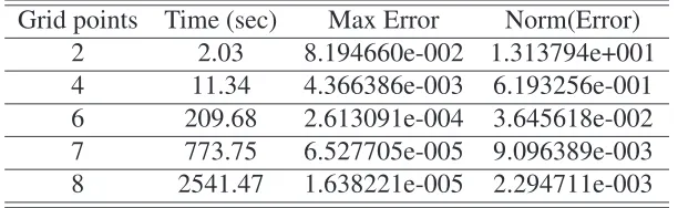
Figure 2 plots the parameterized policy functions for transfers, the continuation value of the agent and the value function of the principal. Transfers are increasing inφ, as is agent’s
lifetime utility. On the contrary, the planner’s value is monotone decreasing and convex in the Pareto weight.
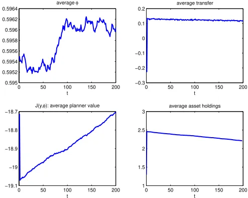
studies: average consumption decreases while average effort increases. As in Thomas and Worrall (1990), the average path for agent’s lifetime utility is decreasing, while the Lagrange
multiplierλis reduced on average along the optimal path. Interestingly, φdoes not show a
monotone pattern. To understand the last plot of Figure 4, notice that it is possible to derive the asset holdings implied by optimal allocations (Appendix C shows the details). According to the simulations, average assets must decrease across time22.
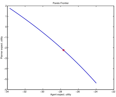
Finally, Figure 5 shows the Pareto frontier: it is decreasing and strictly concave.
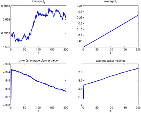
4.2.2 Hidden assets
This is a computed example for the model presented in Appendix B. Functional forms and
parameters are the same as in the previous example, and moreoverβR= 1. Policy functions
for consumption, agent lifetime utility and λ are depicted in Figure 6 and 7, and they are
strictly increasing and concave in both costates, while effort is strictly decreasing and convex. The simulated series in Figure 8 and 9 confirm the results in Abraham and Pavoni: on average, consumption and lifetime utility increase across time, while effort decreases. Asset holdings (see Appendix C to see how they are calculated) also increase on average.
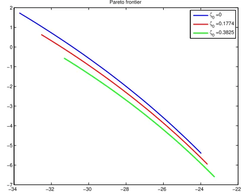
Finally, Figure 10 shows the Pareto frontier for differentζ0 (the natural one is zero): it is
decreasing and strictly concave. An application of the verification procedure described in the Appendix B shows that the first-order approach is justified.
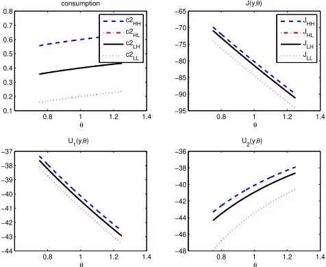
4.2.3 Risk sharing
Two identical agents that must share their income in an endowment economy (hence there are no endogenous state variables). There is two-sided moral hazard: they can exert unobservable effort that affect the future distribution of income realization. In terms of the Proposition 2, letN = 2, ςi ≡ ci,ri(ςi, ai, s)≡ u(ci)−v(ai). Theoretical and numerical results for this
model are analyzed in detail in Mele (2009), therefore I report a synthesis of them.
I solve the model for the case where agents have the same initial weight in the social welfare function, with the same functional forms and parameters of the previous examples, except for income realizations:
αi εi νi σi yiL yiH β ωi
0.5 2 0.5 2 .4 .6 0.95 0.5
It is possible to show that, due to the homogeneity properties of value and policy func-tions, the relevant state variable in this economy is the ratio of endogenous Pareto weights for
agent 1 and 2: θ ≡ φ2
φ1. From the Lagrangean’s first-order conditions I obtainθ =
u′
(c1) u′(c
2) and
it can be shown thatθis a submartingale. The variable θcan be interpreted as a measure of
consumption inequality, and given the submartingale characterization, it should be very per-sistent. These results are in line with theoretical and numerical findings in Zhao (2007) and
Friedman (1998). Figures 11 and 12 show that agent 1’s consumption and lifetime utility are decreasing inθfor any possible state of the world while effort is increasing inθ. Obviously,
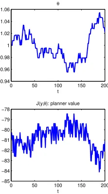
the contrary is true for agent 223. Figure 13 and 14 show a sample path of 200 periods. Notice thatθ is very persistent as expected. Finally, Figure 15 shows a decreasing, strictly concave
Pareto frontier.
4.2.4 Risk sharing in a production economy
This example extends the risk sharing model to a production economy. As for the endowment economy, I present a summary of the results contained in Mele (2009) and I refer the reader to it for more detailed analysis. Each agent can now produce income by using capital. The production function is subject to idiosyncratic productivity shocks, and their distribution is affected by unobservable effort. The law of motion for capital is standard, with depreciation
rate δi. I keep the same functional forms of the risk sharing example, and I choose the
following production function for both agents:
f(kit) =Aitkitρi
whereAtis the productivity shock which is affected by the unobservable effort. The baseline
parameters are summarized in the following table:
αi εi νi σi ALi AHi β ωi δi ρi ki0
0.05 2 0.1 2 0.45 0.55 0.95 0.5 0.06 0.3 3.1
The parametrization was chosen such that the scale of output didn’t differ too much from previous models. Also in this case, we can use the homogeneity properties of value and policy functions to reduce the state space: the relevant state variables are the ratio of Pareto
weights θ ≡ φ2
φ1 and the capital holdings of each agent ki, i = 1,2. The main difference with respect to the endowment economy is that the persistence in consumption inequality has long-run consequences on the optimal path for capital, and therefore on the long-run path for production.
The following simulation results assume that agents are identical and equally weighted at time zero. Figures 16 and 17 show a simulated sample path for this setup. Both consumption and investment are very volatile. Notice also that consumption inequality is very persistent, and this is reflected in the path of expected discounted utilities of each agent.
The average allocations based on 50000 simulations with a horizon of 500 periods are presented in Figure 18 and 19. The main result is the divergence of capital in the long run. This is due to the history dependence of investment: in each period, it is better to invest a little more in the production technology that has a better history of shocks, i.e. the technology of the richest agent. Hence this framework can potentially explain why capital does not flows to countries with higher marginal productivity (see Lucas (1990)): there are financial frictions that are related with private information which make the investment in poor countries less productive. A more detailed analysis is contained in Mele (2009).
23Notice that, given the i.i.d. assumptions on shocks and the fact that shocks for the two agents have the same support, it turns out thatcLH
i =c
HL
4.3
Computational speed and accuracy
The following tables present results for several performance tests. In order to test the com-putational speed of the algorithm and the accuracy of the approximated solution, the codes
solve the examples for different number of grid points. LetM be the number of grid points
in each dimension of the state space, e.g. with three endogenous state variables the grid has a total ofM3 grid points. The general message of this exercise is that it is possible to get an
accurate solution in few seconds even with relatively few grid points. The hardware is a HP Pavilion dv6700 Notebook PC, with a processor Intel Core2 Duo T5450 at 1.66 GHz and 3 GB RAM.
[image:24.595.159.454.378.487.2]The accuracy of the approximated solution can be tested by defining a large grid (with roughly 100000 linearly spaced grid points) and calculating the error of the Lagrangean first-order conditions for each grid point under the approximated solution. In the following tables, there are two statistics that measure accuracy: the maximum error and the norm of the error vector.
Table 1: Speed and Accuracy. Repeated Moral Hazard
Grid points Time (sec) Max Error Norm(Error)
10 4.54 5.468001e-005 1.102151e-002
15 6.23 7.766462e-006 1.830439e-003
20 6.93 2.689196e-006 4.700367e-004
30 8.56 3.956188e-007 8.931410e-005
50 12.38 3.828380e-008 6.437146e-006
100 25.20 3.382069e-009 5.187055e-007
[image:24.595.159.455.585.709.2]Table 1 reports results for the simplest repeated moral hazard model. The computational time is in the order of few seconds, and a fairly good accuracy (i.e., the maximum error is of the order of less than10−5) is obtained with few grid points.
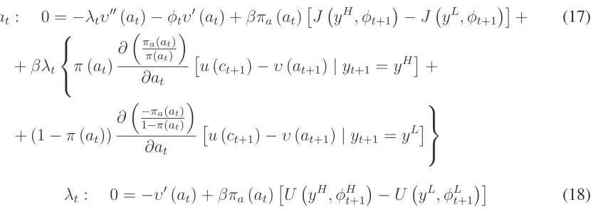
Table 2: Speed and Accuracy. Hidden Assets
Grid points Time (sec) Max Error Norm(Error)
4 3.61 8.185706e-004 1.366256e-001
6 5.70 6.107623e-004 6.481781e-002
8 9.10 1.347988e-004 1.511452e-002
10 13.55 5.534577e-005 5.425800e-003
12 24.80 2.373655e-005 2.409307e-003
15 84.05 7.876450e-006 8.739442e-004
20 132.72 5.343009e-006 3.026376e-004
worth mentioning again that the Fortran code of Abraham and Pavoni (2009) runs for around 15 hours before finding a solution. Therefore, the gain in terms of computational intensity is huge (remember that the code for the Lagrangean approach is written in Matlab, which is a much slower programming language than Fortran).
Table 3: Speed and Accuracy. Risk Sharing, Endowment Economy
Grid points Time (sec) Max Error Norm(Error)
10 5.29 5.181706e-006 8.094645e-004
15 6.92 1.228476e-006 1.589214e-004
20 7.85 4.318931e-007 5.363575e-005
30 9.77 8.595712e-008 1.136224e-005
50 13.92 1.175558e-008 1.166124e-006
100 27.06 5.406727e-008 1.177096e-006
The two-agents risk sharing model in an endowment economy has the same level of dif-ficulty than the standard repeated moral hazard model, as table 3 shows. With 10 grid points,
the maximum error is less than10−5. Again, the computational time is in the order of few
seconds.
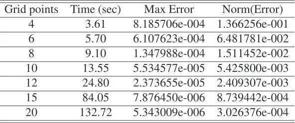
Table 4: Speed and Accuracy. Risk Sharing, Production Economy
Grid points Time (sec) Max Error Norm(Error)
2 2.03 8.194660e-002 1.313794e+001
4 11.34 4.366386e-003 6.193256e-001
6 209.68 2.613091e-004 3.645618e-002
7 773.75 6.527705e-005 9.096389e-003
8 2541.47 1.638221e-005 2.294711e-003
Finally, table 4 presents the statistics for the last example of risk sharing in a production economy. This model has three endogenous state variables, therefore it is more complicated to solve. However, also in this case we do not need a very fine grid to get decent levels of accuracy. Computational time increases, but it is still at tolerable levels (42 minutes with 8 grid points for each dimension). I conjecture that the performance of the algorithm can be improved by combining collocation with the Smolyak algorithm (see for example Malin et al. (2010)). In particular, Smolyak can be useful for more complicated models , since it is well known that the collocation method does not perform well for state spaces with more than 3 endogenous states variables.
5
Discussion
[image:25.595.154.460.440.534.2]5.1
Applicability
The benefits of the approach put forward in this paper are clear at this point: simplicity, tractability and computational speed. The cost that must be paid is a restriction to the class of models that can be analyzed: they must allow the use of the first-order approach. At first, this cost seems large: the conditions for the validity of the FOA are quite restrictive. However, there are many potential applications in macroeconomics that can reasonably be analyzed under these restrictive assumptions.
Take for example optimal unemployment insurance as in Hopenhayn and Nicolini (1997), where a worker looks for a job and his search effort affects the probability of finding it. This model features only two possible realizations of the state of nature: either employed or unemployed. In this case, conditions guaranteeing the validity of the FOA seem quite natural: they imply that more effort changes the distribution of possible outcomes in the sense of first-order stochastic dominance, i.e. more effort increases the probability of finding a job.
More generally, Rogerson (1985b) or Jewitt (1988) conditions can be shown to justify the FOA in models with several agents and/or endogenous observable states. In most of these models, the choice for the researcher is therefore between the analysis of a restricted class of models for which the FOA is valid, or the impossibility to analyze it with the APS approach. The first option seems a valid alternative at least for getting a first idea of the phenomenon under study.
The major concern might be related to models with unobservable endogenous states, for which we still miss a characterization of sufficient conditions that justify FOA. As suggested in the previous sections, these models might be tricky and therefore the recursive Lagrangean techniques must be used with caution, for two reasons: one, even if these models can be easily solved with the algorithm suggested in section 4.1, the solution might not be incentive compatible. Second, it is true that the ex-post verification algorithm can tell if the solution satisfies incentive compatibility. However, it should be thought as a tool for validating the use of FOA when one has already a reasonable expectation that FOA would work. It is indeed a risky strategy to start using the Lagrangean approach just to discover later on that the FOA is not valid in that particular application or with that particular calibration.
Nevertheless, the recent work of Abraham, Koehne and Pavoni (forthcoming) on two-period repeated moral hazard with hidden savings suggests a proof strategy for the validity of FOA in multiperiod models that could potentially be pursued for specific applications. This is an interesting possibility that is out of the scope of this paper, and therefore it is left for future research.
5.2
Local vs global
This problem can be addressed if one is ready to compromise speed with global results. The suggested algorithm is not the only way to find a solution. The main benefit of the algo-rithm is its speed and the simple implementation, however the big advantage of the recursive Lagrangean approach (the absence of a characterization step for the feasible set of costate variables) does not depend on it. If one has a strong reason to believe that the Kuhn-Tucker conditions are not sufficient, the saddle point can be found by iterating over the value func-tion and using a global optimizafunc-tion procedure (e.g., direct search or genetic algorithms). While this computational strategy would loose the gains in terms of speed, it still retains the advantage of not needing a characterization of the costates’ feasible set.
6
Conclusions
The use of recursive Lagrangeans as a solution strategy is common for dynamic environment with full information, but not for private information setups. Sleet and Yeltekin (2008a) open the way for applications with privately observed shocks. This paper does the same for models with privately observed actions, and in particular proposes an algorithm which is much faster than the traditional APS technique. This methodology allows the researcher to deal with models with many states, and to calibrate simulated series to real data in a reasonable amount of time. A large class of models which are practically intractable under standard techniques can be easily addressed with the techniques discussed here.
This method has many possible applications. Given the speed, the algorithm can also be useful (as a time-saving technique) for solving those models that are tractable with tra-ditional techniques, but computationally burdensome. These techniques can be potentially helpful in the analysis of several issues such as e.g. consumption-saving anomalies, optimal unemployment insurance with assets accumulation or DSGE models with financial frictions. However, the main gain of the Lagrangean method can be seen in more complicated setups, which are practically intractable with current state-of-the-art algorithms. Models of repeated moral hazard with heterogeneous agents and endogenous states are a good example: they require us to solve the problem of each agent and aggregate the resulting individual optimal choices, before iterating until a general equilibrium is found. In these cases, APS techniques are unmanageable even with just two endogenous states, while with my approach it is a simple computational task. Other problems for which the Lagrangean approach has a potential advantage are optimal taxation theory in economies with hidden effort and several assets, models of CEO compensation, and models of banking and credit markets.