Effectively Using the QRFM to Model Truck Trips in
Medium-Sized Urban Communities
Michael D. Anderson1, Mary C. Dondapati1, Gregory A. Harris2
1Department of Civil and Environmental Engineering, University of Alabama in Huntsville, Huntsville, USA 2Center for Management and Economic Research, University of Alabama in Huntsville, Huntsville, USA
Email: [email protected]
Received March 21, 2013; revised April 22, 2013; accepted April 30, 2013
Copyright © 2013 Michael D. Anderson et al. This is an open access article distributed under the Creative Commons Attribution License, which permits unrestricted use, distribution, and reproduction in any medium, provided the original work is properly cited.
ABSTRACT
This paper analyses the effectiveness of applying the Quick Response Freight Manual (QRFM) to model freight trans-portation. Typically, freight transportation is indirectly modeled or as an after-thought. Increasing freight volumes, cou-pled with cost saving strategies such as just-in-time delivery systems, require that transportation policymakers analyze infrastructure needs and make investment decisions that explicitly include freight volumes as a component. This paper contains a case study using a medium sized urban area travel model and the QRFM trip generation and a distribution methodology to provide a framework for freight planning that can be used to improve resource allocation decisions.
Keywords: Freight Modeling; Travel Demand Modeling
1. Introduction
The efficient and effective movement of freight is a critical component in the transformation and growth of the economy. Often, transportation planners use urban transportation planning models, which are representa-tions of the existing transportation infrastructure to de-termine the impacts of future changes. These planning models are developed and validated to reflect existing traffic volumes and patterns. After validation, the models are used for forecasting daily traffic volumes on primary arterials and freeways and evaluate changes in roadway infrastructure and socio-economic characteristics. In small and medium sized urban communities, proper roadway infrastructure resource allocation decisions based on data obtained from the community’s travel de-mand model and long-range transportation planning process could potentially be the determining factor be-tween continued community growth and stagnation.
Since the modeling process is important, it is critical that the models used provide the best forecasts of future conditions. Unfortunately, freight transportation require- ments are often not included in travel demand models developed and maintained in small communities, or else, freight trips are included in these models through very simplified methodologies.
This paper examines the potential to use available freight trip generation factors and a distribution scheme
to determine freight transportation demand appropriate for incorporation into a community travel demand model. First, the paper presents background into travel demand forecasting and the Quick Response Freight Manual (QRFM) trip generation equations [1,2]. Next, the paper applies the model through a case study of Huntsville, AL, a medium-sized community in the north-central portion of the state. A statistical analysis of the QRFM technique is applied to the network using a variety of distribution schemes to improve its forecasting ability. The paper concludes that the proper incorporation of freight trans-portation needs into the travel demand modeling process can improve its results and should lead to improved in-vestment decisions for the community.
2. Transportation Planning Background and
Freight Specifics
transportation, factors that can influence trips produced from or attracted to a zone are: household income and size, automobile ownership, type of businesses, and trip purpose [3]. The trip generation step then converts these zonal data values into trip purposes. However, in most small and medium sized urban communities, there is no model developed for freight productions or attractions since it is time consuming and costly to survey busi-nesses and manufacturers on their specific freight re-quirements.
Trip distribution connects trip origins and destinations for the development of a trip interchange matrix. The two main factors considered are trip length and the travel direction or orientation. The most common method used for trip distribution is a gravity model, which is based on Newton’s law [3]. The gravity model predicts that trip interchanges between zones are directly proportional to the productions and attractions in the zones and inversely proportional to the spatial separation between zones [3]. In other words, zones with more activities or businesses are more likely to exchange more trips, and zones with longer distances between them are likely to exchange fewer trips. For freight, it is expected that the trip distri-bution would be similarly performed.
Modal split is used to estimate how many trips will use public transit and how many trips will use private vehi-cles, typically using a logit model [3]. However, this step of the process is generally ignored in small and medium sized communities, as transit ridership is not significant. With freight however, this step would contrast truck versus alternative modes of shipment (rail, water, and air) and therefore it is significant. As limited availability for alternate freight shipping models often exists in medium sized communities, this step is still not included in the modeling process.
Traffic from the modal split analysis is then assigned to available roadways or transit routes using Waldrop’s equilibrium theorem, or some approximation of equilib-rium. By this theory, under equilibrium conditions traffic arranges itself in congested networks in such a way that
no individual trip maker can reduce his path costs by switching routes [3]. Regarding freight, it is not neces-sarily logical to assume freight shipments will likely change their route due to congestion effects, at least not off the major roadways within the communities.
To overcome the absence of freight in transportation models, the original Quick Response Freight Manual (QRFM) and its updated version QRFM II, were pre-pared for the Federal Highway Administration [1,2]. The objective of the reports were to provide background in-formation on the freight transportation system and factors affecting freight demand to planners who may be rela-tively new to the inclusion of freight planning and to provide simple techniques and transferable parameters that can be used to develop commercial vehicle trip ta-bles which can then be merged with passenger vehicle trip tables developed through the conventional four-step planning process. The QRFM report identifies trip gen-eration factors that define production and attraction val-ues manageable within a small community. To support trip distribution, the QRFM provides a series of friction factors that can be incorporated into the gravity model to specify the expected length of freight movements. Fig-ure 1 provides the trip generation equations and Figure 2 the friction factor equations.
3. Case Study: Huntsville, AL
Huntsville, Alabama with a population of approximately 300,000 was selected as case study to analyze the incor-poration of freight into the modeling process. For this research, the data on the transportation network for the City of Huntsville was acquired from the Huntsville Metropolitan Planning Organization (MPO); see Figure 3 [4].
The research was performed by applying the trip gen-eration rates obtained from the QRFM to the socio-eco- nomic data collected by the Huntsville MPO. For each zone, the socio-economic data were converted into freight trips using the rates provided by the QRFM. A
Commercial Vehicle Trip Destinations (or Origins) per Unit per Day Generator
Four-Tire Vehicles Single Unit Trucks (6 + Tires) Combinations TOTAL
Employment
Agriculture, Mining and Construction 1.110 0.289 0.174 1.573
Manufacturing, Transportation, Communications,
Utilities and Wholesale Trade 0.938 0.242 0.104 1.284
Retail Trade 0.888 0.253 0.085 1.206
Office and Services 0.437 0.068 0.009 0.514
[image:2.595.60.538.581.721.2] Households 0.251 0.099 0.028 0.388
Figure 2. Friction factors from the original QRFM. (Source Cambridge Systematics, Inc. Quick Response Freight Man-ual II. Federal Highway Administration. Publication No. FHWA-HOP-08-010. September 2007).
Figure 3. Huntsville, AL planning model.
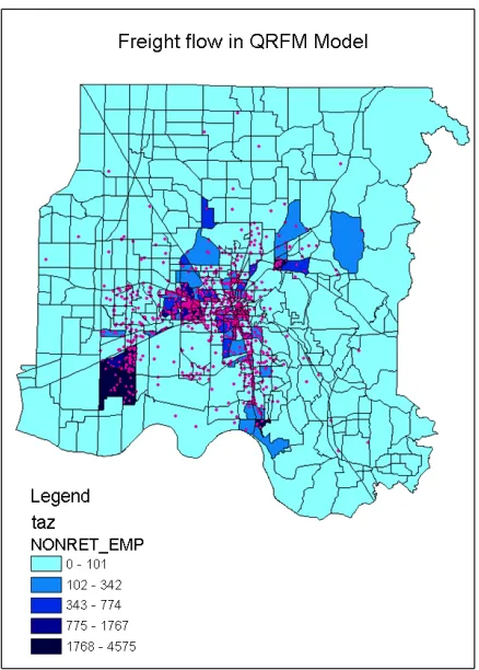
visual validation of the trip generation model results as they related to the total non-retail employment in the study city was performed by developing a thematic map showing the amount of non-retail employment within each traffic analysis zone overlaid with a dot density plot of the freight trips (see Figure 4). The figure indicated that the QRFM freight trips were located in areas of higher non-retail employment. This result was expected and validated the use of the QRFM model in the planning process.
The Huntsville model was based on trip generation, distribution and assignment. Common with the practice in planning studies this model used the static traffic as-signment technique. The rationale is that it mirrored the current modeling system used in the community and ap-proved by the state for transportation forecasting proc-esses. This ensured that the model would be accepted
Figure 4. Freight trips versus non-retail employment.
upon development of a successful application. Though not used, the analysis could have benefitted by employ-ing dynamic traffic assignment techniques, such as those available in PARAMICS, VISSUM or VISTA, that have the capability to move vehicles through the network us-ing car followus-ing and lane changus-ing models [5].
4. Statistical Analysis
[image:3.595.63.282.293.510.2]possibil-ity exists for some trucks to be assigned to local road-ways, the number of such trucks is assumed to be mini-mal.
The accuracy of the assignment of truck volumes was determined by comparing the assignment results to the actual truck volumes reported by Alabama Department of Transportation (ALDOT). The first comparison used a scatter plot of actual truck traffic volume versus traffic volumes from the QRFM. That plot in Figure 5 shows that there is no clear relationship between the QRFM results and the actual freight counts in Huntsville using the 100% internal distribution.
To statistically measure the difference between the as-signed truck traffic and actual truck counts, the Nash-
Sutcliffe (NS) coefficient was calculated [6]. The value of this coefficient ranges from −∞ to 1, with a coefficient of one (E = 1) showing a perfect match of forecasted
counts to the ground counts. A zero coefficient (E = 0)
shows that the forecasted values are as accurate as the mean of the ground counts, whereas a coefficient less than zero (−∞ < E < 0) occurs when the forecasted mean
is less than the ground counts. In other words, this coef-ficient gives a measure of scatter variation from the 1:1 slope line of modeled truck counts versus the ground counts. The more deviation of points from the 1:1 slope line, the lower the coefficient. The greater the NS-value the better is the forecast. This coefficient can be calcu-lated using the formula:
2n n
1 1
NS 1
Modeled Counts Ground Counts
Ground Counts Mean Ground CountsThe application of the Nash-Sutcliffe test to the data gave an efficiency coefficient of −1.45 showing that tak-ing an average value of the truck counts from ALDOT would better predict truck flows than the travel demand model.
Further statistical tests were performed to determine whether the data obtained from the travel demand model were similar to actual truck counts. The MINITAB™ statistical software was used to conduct the analysis of variance (ANOVA) test. The results provide statistical evidence to suggest that actual truck volumes are differ-ent from the volumes assigned by the model.
To improve the results, an alternate trip distribution method was employed. This method was developed from the results of a study being done in Mobile, Alabama [7]. The flow patterns collected from the Mobile area in Ta-ble 1 show that external-internal (E-I) truck trips and internal-external (I-E) truck trips represent over 80% of
Model Volumes Versus Truck Counts (100% Internal Trips)
0 500 1000 1500 2000 2500
0 500 1000 1500 2000 2500 3000 3500
Truck Count
M
od
e
l A
s
s
ign
m
e
[image:4.595.59.288.529.716.2]nt
Figure 5. Scatter plot of truck traffic.
the total truck volumes, while the internal-internal (I-I) truck trips account for less than 20%. This implies that approximately 80% of the raw materials for manufactur-ing are generated outside the area, and approximately 80% of the finished products are exported to points out-side the area.
To account for changes in truck distribution in the model, the modules used to run the Huntsville MPO travel demand model were adjusted to account for freight trips distributed into the community from outside (E-I), and outward from the community to points beyond the study area (I-E). An experiment was designed to include four different trip distribution levels:
90% (E-I and I-E) and 10% (I-I),
80% (E-I and I-E) and 20% (I-I),
70% (E-I and I-E) and 30% (I-I), and
60% (E-I and I-E) and 40% (I-I).
The reason for not simply using the 80% E-I and I-E found in the Mobile project is the uncertainty that Hunts-ville would perform similarly as Mobile due to socio- economic differences in the two communities and the influence of the Port of Mobile.
[image:4.595.310.538.652.735.2]The E-I and I-E truck trip distributions were developed using the total number of trucks crossing the study area boundary. The total number of trucks at the boundaries was split by percentage into the number of trucks ex-pected to enter and leave the community (E-I and I-E)
Table 1. Freight locations for mobile area.
Freight Origin/Destination
Location Origins Destinations
Within Mobile County 14.5% 16.4%
Outside Mobile County 84.5% 80.7%
and the number of trucks passing through the community. Parameters in the gravity model were set to constrain the E-I and I-E truck numbers such that the total number of trucks at the external stations did not exceed boundary conditions. A separate gravity model, which used the modeling details for the City of Huntsville, was used for the internal truck trips that included a reduction factor to limit the number of trips. As before, mode split was not included in the model and truck trips were assigned to the Huntsville network without passenger cars to allow truck access to the major roadways.
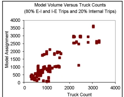
A scatter plot was drawn to compare actual truck count and the trucks assigned from the model for each per-centage split. A scatter plot for the 80% E-I and I-E with 20% internal trips is shown in Figure 6. As can be seen, the results appear to align much closer to the 1:1 slope with the trip distribution adjustment.
For comparison, the Nash-Sutcliffe efficiency coeffi-cient was calculated for each trip distribution split. The results were as follow:
NS Coefficient = 0.59 for the 90% (E-I and I-E) and 10% (I-I),
NS Coefficient = 0.61 for the 80% (E-I and I-E) and 20% (I-I),
NS Coefficient = 0.62 for the 70% (E-I and I-E) and 30% (I-I), and
NS Coefficient = 0.61 for the 60% percent (E-I and I-E) and 40% (I-I).
As these results show, there is little difference between the models. However, all the models show significant improvements over the 100% internal distribution.
[image:5.595.69.274.549.709.2]Further statistical tests were performed to determine if the data obtained from the travel demand model were similar to actual truck counts. MINITAB™ Statistical Software was used to analyze the data and to perform the analysis of variance (ANOVA) test. The results show no statistical evidence that actual truck volumes are different from the volumes assigned by the model. Further, using
Figure 6. Scatter plot of truck traffic with distribution mo- dification.
the Mann-Whitney non-parametric test, it is found that that the QRFM data likely come from the same popula-tion as the actual data.
The implementation of the methodology would require that smaller communities develop a truck trip purpose using the QRFM equations. However, the resulting truck values need to be converted into internal truck trips and internal-external and external-internal truck trips based on the percent trips expected to leave the study area. Then, the two purposes need to be included into the modeling process as would be followed using any num-ber of trip purposes.
5. Statistical Analysis
This paper demonstrated that trip generation equations from the QRFM, when calculated using socio-economic data from a medium sized travel demand model, can ac-curately reflect the locations where truck trips are likely to originate or terminate inside a community. Secondar-ily, this paper showed that the use of an appropriate trip distribution method that accounts for freight movements entering and leaving the study area produces an accurate forecast of trucks on existing roadway infrastructure, the percent values to use will be based on varying the data and determining the best fit or using the recommended values presented in this paper. This ability to successfully model freight in an urban area can be used to overcome the limitation of neglecting freight in travel demand modeling processes.
REFERENCES
[1] Cambridge Systematics, Inc., “Quick Response Freight Manual,” Federal Highway Administration, Washington DC, 1996.
[2] Cambridge Systematics, Inc., “Quick Response Freight Manual II,” Federal Highway Administration, Washing- ton DC, 2007.
[3] J. de Dois Ortuzar and L. G. Willumsen, “Modeling Trans-port,” 2nd Edition, John Wiley and Sons, New York, 1994. [4] Huntsville MPO (Metropolitan Planning Organization),
“Information Provided by Mr. James Moore, Transporta- tion Planner for Huntsville,” AL Metropolitan Planning Organization, Decatur, 2007.
[5] M. Jeihani, “A Review of Dynamic Traffic Assignment Computer Packages,” Journal of the Transportation Re- search Forum, Vol. 46, No. 2, 2007, pp. 35-46.
[6] J. E. Nash and J. V. Sutcliffe, “River Flow Forecasting Through Conceptual Models Part I: A Discussion of Principles.” Journal of Hydrology, Vol. 10, No. 3, 1970, pp. 282-290. doi:10.1016/0022-1694(70)90255-6
![Figure 1. Trip generation rates from the QRFM [2].](https://thumb-us.123doks.com/thumbv2/123dok_us/7785450.723360/2.595.60.538.581.721/figure-trip-generation-rates-qrfm.webp)