What is the actual shape of perception utility?

Munich Personal RePEc Archive

What is the actual shape of perception

utility?

Kontek, Krzysztof

Artal Investments

20 June 2011

Online at

https://mpra.ub.uni-muenchen.de/31715/

What is the Actual Shape of Perception Utility?

Krzysztof Kontek1

Abstract

Cumulative Prospect Theory (Kahneman, Tversky, 1979, 1992) holds that the value func!

tion is described using a power function, and is concave for gains and convex for losses. These

postulates are questioned on the basis of recently reported experiments, paradoxes (gain!loss se!

parability violation), and brain activity research. This paper puts forward the hypothesis that per!

ception utility is generally logarithmic in shape for both gains and losses, and only happens to be

convex for losses when gains are not present in the problem context. This leads to a different

evaluation of mixed prospects than is the case with Prospect Theory: losses are evaluated using a

concave, rather than a convex, utility function. In this context, loss aversion appears to be nothing

more than the result of applying a logarithmic utility function over the entire outcome domain.

Importantly, the hypothesis enables a link to be established between perception utility and Portfo!

lio Theory (Markowitz, 1952A). This is not possible in the case of the Prospect Theory value

function due its shape at the origin.

JEL Classification: C91, D03, D81, D87, G11.

Keywords: Prospect Theory, value function, perception utility, loss aversion, gain!loss separabil!

ity violation, neuroscience, Portfolio Theory, Decision Utility Theory.

1

Introduction

Prospect Theory (Kahneman, Tversky, 1979) postulates that the value function is concave

for gains and convex for losses. This implies that people are risk averse for gains and risk seeking

for losses. The theory also presents loss aversion as a separate phenomenon. This reflects the

greater weight assigned to losses than to gains of the same size. The cumulative version of the

theory (Tversky, Kahneman, 1992) describes the value function using a power function with a

1

power coefficient α of 0.88 for both gains and losses. Loss aversion is modeled using a coeffi!

cient of λ = 2.25, meaning that people are more than twice as sensitive to losses as they are to

gains. The theory further assumes that gains and losses are evaluated separately using respective

value and probability weighting functions, and that the prospect value is the sum of the two.

These well known postulates are confronted in this paper with recent experimental results.

It turns out that a power function, reflecting “preference homogeneity” (Tversky, Kahneman,

1992), leads to surprising failures in interpreting lotteries with increasing stakes (Point 2). Not

only that, it makes it impossible to explain several well known paradoxes, such as the original Al!

lais paradox simultaneously with participation in lotteries (Neilson and Stowe, 2002) and the St.

Petersburg Paradox (Blavatskyy, 2005).

Despite increasing experimental evidence, there is additionally no consensus as to whether

utility is convex or concave for losses (Point 3). Most people exhibit risk seeking behavior, but a

strong minority (25% to 50%) behave in an opposite manner. Moreover, the Cumulative Prospect

Theory conclusion that people are risk seeking for loss prospects appears to be merely the acci!

dental result of using a specific form of the probability weighting function to estimate the power

coefficient of the value function.

On the other hand, loss aversion appears to result from a single process which governs

losses and gains (Point 4); it has been shown that potential losses and gains trigger decreas!

ing/increasing activity in the same region of the brain (Tom, 2007). A premise of Prospect The!

ory regarding the separate valuation of gains and losses is also questioned (Point 6). Experimental

studies demonstrate a systematic violation of the double matching axiom, an axiom that is neces!

sary for gain!loss separability (Wu, Markle, 2008; Birnbaum, 2007).

A new hypothesis is put forward in Point 5 of this paper to resolve these inconsistencies. It

holds that utility is generally logarithmic in shape and only happens to be convex when gains are

absent in the problem context. According to this hypothesis, a logarithmic perception of losses

and gains is the default process and any “reflection” of the utility curve for losses is merely an

exception to the rule. Several arguments confirming this statement are presented. The hypothesis

easily explains gain!loss separability violations and leads to a different evaluation of mixed pros!

pects than that postulated by Cumulative Prospect Theory. Loss aversion appears to be simply the

result of applying a logarithmic utility function to both losses and gains.

ferences with the Prospect Theory value function. The similarities should also be pointed out. In

principle, they are the both psychophysical functions defined relative to a reference point. In the

original Prospect Theory paper (1979) Kahneman and Tversky state: “Many sensory and percep

tual dimensions share the property that the psychological response is a concave function of the

magnitude of physical change. For example, it is easier to discriminate between a change of 3°

and a change of 6° in room temperature, than it is to discriminate between a change of 13° and a

change of 16°. We propose that the value function which is derived from risky choices shares the

same characteristics”.

The perception utility function and the value function are essentially the same concepts.

This paper shows, however, that the two functions differ in almost every respect: the functional

forms used to describe them, the loss aversion concept, and finally the shape for losses and gains

considered separately and jointly. As stated in the discussion (Point 7) the hypothesis enables a

link to be established between perception utility and Portfolio Theory (Markowitz, 1952A). This

is because the logarithmic function can be well approximated around 0 using the quadratic func!

tion, which is the basic assumption required to transpose the expected utility considerations into

the return!risk plane. This transposition is not possible in case of the Prospect Theory value func!

tion due to its shape at the origin.

2

Functional Form

2.1 Power Function

Let us suppose that somebody is indifferent between a certain $40 and a 50% chance of

winning $100. The ratio of the certainty equivalent ce to the lottery outcome P is 40/100 = 0.4 in

this case. This ratio should decrease when P becomes very large: a subject will definitely expect

much less than a certain $40 million when confronted with a 50% chance of winning $100 mil!

lion.

It is commonly believed these sorts of behaviors can be explained by Prospect Theory,

more specifically by the shape of its value function. Kahneman and Tversky (1979) noticed: “The

difference in value between a gain of 100 and a gain of 200 appears to be greater than the differ

ence between a gain of 1,100 and a gain of 1,200. Similarly, the difference between a loss of 100

unless the larger loss is intolerable. Thus, we hypothesize that the value function for changes of

wealth is normally concave above the reference point and often convex below it. That is, the mar

ginal value of both gains and losses generally decreases with their magnitude”. Quite surpris!

ingly, Cumulative Prospect Theory fails to explain the case considered. The theory assumes that

the value function is described by a power function that conforms to Stevens Law (1957), i.e.:

( )

v x =xα (2.1)

According to this theory, the weight w associated with probability p is constant. It follows

that the indifference in the first case is described as:

( )

40α =100αw 0.5 (2.2)

Multiplying both sides of (2.2) by a constant 1,000,000α we obtain:

( )

40, 000,000α =100, 000, 000αw 0.5 (2.3)

which describes the indifference between a certain $40 million and a 50% chance of winning

$100 million. This means that proportional increasing lottery stakes does not change the prefer!

ence. This property of Cumulative Prospect Theory is not accidental; Tversky and Kahneman

(1992) refer to it as “preference homogeneity”. The obvious failure of the theory in the consid!

ered case can be described in a more general way. The certainty equivalent is obtained by apply!

ing the formula:

( )

( ) ( )

v ce =v P w p (2.4)

As the value function is assumed to be a power function, the following holds:

( )

ceα =P w pα (2.5)

Hence

( )

w p P P α α α   = _{=  }

  (2.6)

and

( )

ce

w p P

α

= (2.7)

It follows that the ce/P ratio is constant for a given shape of the probability weighting

function w, and a given power coefficient α of the value function. Cumulative Prospect Theory

can only explain a change in preference in terms of a change in either the probability weighting

the fundamental Prospect Theory assumption that probability weighting is an independent “psy!

chological” phenomenon. The second condition would imply a break in “preference homogene!

ity”. This would require a utility curve where relative risk aversion increases with outcome size,

but this in turn would automatically exclude the power function from the list of possible func!

tional form candidates.

The inability of the power function to explain this particular case might account for the

other documented Cumulative Prospect Theory failures. Neilson and Stowe (2002) demonstrate

that Cumulative Prospect Theory cannot simultaneously explain participation in lotteries and the

original Allais paradox. Although the authors looked at different forms of the probability weight!

ing function, they only considered the power value function. Blavatskyy (2005) similarly demon!

strated that Cumulative Prospect Theory, with its power value function, cannot explain the St. Pe!

tersburg Paradox.

2.2 Logarithmic Function

Bernoulli stated that the St. Petersburg Paradox could be explained using logarithmic utility

as early as 1738. This solution works even when probability weights are applied. Similarly, it can

be verified that the original Allais Paradox can be explained together with the gambling using

logarithms of outcomes. Scholten & Read (2010) considered similar patterns by verifying the

Markowitz hypothesis regarding the utility shape (1952B). They stated that Prospect Theory

could only explain preference change by assuming a value function of decreasing elasticity, in!

stead of the power function, which is of constant elasticity. They proposed using the logarithmic

function v(x) = 1/a ln(1 + a x).

Logarithmic perception is well known due to a fundamental law of psychophysics known

as the Weber!Fechner law. Hearing described using the decibel scale is an example of this sort of

perception. This law, however, has been severely criticized by Stevens (1957), who claimed that

the power function better describes people’s perception. This way it was implemented in Prospect

Theory. In any case, the evidence presented here shows that the power function is unable to ex!

plain many behaviors and paradoxes, whereas the logarithmic function can do this without any

3

Perception Utility for Losses

3.1 Utility Reflection

Kahneman and Tversky (1979) observed the following behavior when making risky deci!

sions: for low probabilities, people are risk seeking for gains, and risk averse for losses, whereas

for high probabilities, they are risk averse for gains and risk seeking for losses. This reversed pat!

tern, which they called the “reflection effect”, supported their hypothesis regarding the convex!

concave shape of the value function.

It should, however, be pointed out that the “reflection effect” does not necessarily imply a

reverse shape of the value function. According to Prospect Theory, probability weighting typi!

cally has a stronger impact on risky decisions than does the utility shape. The theory thus ex!

plains gambling despite the concave utility function for gains. Risky decisions for losses can li!

kewise be explained, even when a moderately concave utility function is assumed. Such utility

would only attenuate the risk seeking attitude postulated by the probability weighting function for

high probabilities. In any case, the convex!concave shape of the value function remained one of

the main postulates of Prospect Theory.

The appearance of the cumulative version of Prospect Theory seemed to confirm this as!

sumption. Tversky and Kahneman (1992) derived a power coefficient of 0.88 for both gains and

losses using experimental data. This implies concavity for gains and convexity for losses – ex!

actly what the original Prospect Theory predicted.

3.2 Mixed Evidence for Losses

Although the value function is well documented to be concave for gains, it is, however,

not all that clear that it is convex for losses, as postulated by Prospect Theory. Van de Kuilen in

his dissertation (2007) summarizes the research on the subject: “First of all, there is no consensus

at present about the fundamental question whether the utility function for losses is convex or con

cave. Some studies found concave utility for losses (Davidson, Suppes & Siegel 1957; Laury &

Holt 2000 (for real incentives only)), while other studies found convex utility for losses (Currim

& Sarin 1989; Tversky & Kahneman 1992; Abdellaoui 2000; Etchart Vincent 2004). Second,

for losses than concavity for gains (Fishburn & Kochenberger 1979; Abdellaoui, Bleichrodt &

Paraschiv 2004), and this constitutes another point of debate since other studies found that con

vexity for losses is less pronounced than concavity for gains (Fennema & van Assen 1999; Köb

berling, Schwieren & Wakker 2004; Abdellaoui, Vosmann & Weber, 2005). Finally, there is no

consensus on whether utility curvature is more (or less) pronounced for larger outcomes. In

creasing relative risk aversion has been found, for example, by Kachelmeier & Shehata (1992),

Holt & Laury (2002, 2005), and Harrison, Johnson, McInnes & Rustrom (2003), whereas the

opposite result, i.e. a decreasing relative risk aversion coefficient, has been found, for example,

by Friend & Blume (1979), and Blake (1996)”.

Other research, not listed above, shows that either convexity prevails (Pennings and

Smidts, 2003), or that the utility is concave (Fehr!Duhda et al. 2006). Also in Lattimore, Baker

and Witte (1992), most individuals’ utility functions appear to be either concave or linear. Libby

and Fishburn (1977) and Laughhunn, Payne and Crum (1980) state that even though decision

makers appear partial to risk in the loss domain, they tend to become risk averse as the losses at

stake become large. A similar pattern was observed by Etchart!Vincent (2009): “Even though

most elicited individual utility functions classically appear to be either concave or convex (most

of them being convex), a strong minority of them (25%) tends to exhibit a concave convex shape,

with convexity over moderate losses changing to concavity as losses grow”. Even more complex

patterns were described by Scholten and Read (2010), who replicated the Markowitz (1952B) ex!

periment: “For gains, most people change from risk seeking to risk aversion as the stakes in

crease, consistent with Markowitz’s hypothesis. For losses, the results are diverse: Some change

from risk aversion to risk seeking, others change in the opposite direction, and still others are

globally risk averse”.

Abdellaoui et al. (2007) summarized recent research: “At the aggregate level, all (authors)

found slightly convex utility for losses (median power coefficients vary between 0.84 and 0.97). At

the individual level, the most common pattern was convex utility for losses (between 24% and

47% of the subjects), but concave and linear utility functions were also common”. The authors

presented their own results which indicated a slight convexity for losses. However, Abdellaoui et

al. (2008) presented other research which contradicted their previous conclusion. The power co!

3.3 Are People Really Risk Seeking for Losses?

The differences between these conclusions may partially be accounted for by the experi!

mental design and data analysis method used. We will demonstrate that the Cumulative Prospect

Theory conclusion that people are risk seeking for loss prospects appears to be merely an acci!

dental result of using a specific form of the probability weighting function to estimate the power

factor of the value function.

A standard nonlinear regression procedure was applied to the experimental data presented

in the Cumulative Prospect Theory paper (1992). Using the functional form of the probability

weighting function postulated by Cumulative Prospect Theory results in parameter values α =

0.906 and δ = 0.704. These values are similar to those presented by Cumulative Prospect Theory

(α = 0.88 and δ = 0.69). The power factor α being less than 1 implies the convexity of the value

function for losses, and would mean that people are risk seeking in this case.

The drawback of the form proposed by Cumulative Prospect Theory is that it only has a

single parameter to model the shape of the probability weighting function. More flexible, two–

parameter functions have been used to check whether the functional form of the probability

weighting function has an impact on the result of the power factor estimation (γ and δ denote pa!

rameters):

a). The form used by Gonzales and Wu (1999)

(

)

p GW

p p

γ

γ γ

δ δ

=

+ − (3.1)

b). The form proposed by Prelec (1998)

( lnp)

PR=e− −δ γ (3.2)

c). Cumulative Beta Distribution

(

)

p

BT =I δ γ (3.3)

where I denotes the beta regularized function.

d). Cumulative Kumaraswamy Distribution

(

)

1 1

KM = − − pδ γ (3.4)

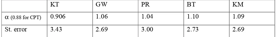
KT GW PR BT KM

α(0.88 for CPT) 0.906 1.06 1.04 1.10 1.09

St. error 3.43 2.69 3.00 2.73 2.69

Table 3.1 Estimation of α for loss prospects using different forms of the probability weighting function with

the corresponding standard errors of certainty equivalent estimation.

As presented, the power factor is only ever less than 1 when the form of the probability

weighting function proposed by Cumulative Prospect Theory is used. In every other case, it is

greater than 1. As shown, the standard error of estimation is greatest in the case of the function

proposed by CPT. Using other forms results in much lower errors, indicating that these models

better fit the experimental data and that their estimations of α are more reliable.

This result demonstrates that the “reflection” of the value function is not confirmed by the

CPT experimental data. The value function appears to be concave for losses (similarly as for

gains), once more flexible functions are used to model the probability weighting function. It fol!

lows that people are generally risk averse both for gains and for losses. This contradicts one of

the fundamental claims of Prospect Theory.

This result not only presents a different interpretation of the Cumulative Prospect Theory

data, it confirms the general conclusion that very different behaviors are observed in the loss do!

main. The nature of this phenomenon has never been satisfactorily explained. We shall attempt to

remedy this in the following points

4

Loss Aversion

Loss aversion plays a central role in Prospect Theory and reflects the fact that people

weigh losses more heavily than gains of the same size. As a result, the utility function, defined

over gains and losses relative to a reference point, presents a kink at the origin with the slope of

the loss function steeper than that of the gain function. The ratio of these slopes at the origin is a

measure of loss aversion. This ratio is generally found to be between 1 and 2.5 with an average

value in the neighborhood of 2 (Tversky and Kahneman 1991, Kahneman, Knetsch, and Thaler

1990, Abdellaoui et al., 2007, Booij & van de Kuilen, 2006; Tversky & Kahneman, 1992). Peo!

ple are thus approximately twice as sensitive to losses than they are to absolutely commensurate

gains.

of loss aversion. There are, however, several psychological and neural explanations. For example,

Litt et al. (2008) state that loss aversion can be explained by “the combination of arousal modula

tion of subjective valuation and the increased affective import of losses (which) produces emo

tionally influenced orbitofrontal valuations that overweight losses”. Several brain imaging studies

have suggested that higher sensitivity to loss is due to emotional processes being triggered in cer!

tain parts of the brain such as the amygdala and the anterior insula. For instance Yacubian et al.

(2006) were “able to confirm ventral striatal responses permitting the local computation of ex

pected value. However, the ventral striatum only represented the gain related part of expected

value. In contrast, loss related expected value was represented in the amygdala”.

A different view was presented by Tom et al. (2007) who examined mixed lotteries to

check whether loss aversion reflects the engagement of distinct emotional processes for potential

losses: “If loss aversion is driven by a negative affective response (e.g. fear, vigilance, discom

fort), then one would expect increasing activity in brain regions associated with these emotions

as the size of the potential loss increases. Contrary to this prediction, no brain regions showed

significantly increasing activation”. The authors further stated that “a broad set of areas showed

increasing activity as potential gains increased. Potential losses were represented by decreasing

activity in several of these same gain sensitive areas. (This) demonstrates that potential losses

are represented by decreasing activity in regions that seem to code for subjective value rather

than by increasing activity in regions associated with negative emotions”. This suggests that a

single process is responsible for loss aversion.

McGraw et al. (Kahneman among them) offer an interesting insight into loss aversion in

their paper “Comparing gains and losses”(2010): “Loss aversion in choice is commonly assumed

to arise from the anticipation that losses have a greater effect on feelings than gains, but evi

dence for this assumption in research on judged feelings is mixed. Many situations in which peo

ple judge and express their feelings lack these features. We argue that loss aversion is present in

judged feelings when people compare gains and losses and assess them on a common scale.

When gains and losses are not context for each other, and people can avoid the comparison en

tirely, the asymmetry fails to appear”. This conclusion can be interpreted as follows. Losses are

evaluated differently for mixed and loss prospects. In mixed prospects, gains are present, and loss

5

Perception Utility Hypothesis

The evidence presented in the preceding points inevitably leads to the conclusion that the

single mechanism responsible for loss aversion might be simply the logarithmic perception of

stimuli. Please note that in logarithmic terms, a 100% profit corresponds to a 50% loss, which

would result in a sensitivity to losses twice as great as that to gains.

Using a logarithmic function to assess both gains and losses can therefore explain the loss

aversion effect and obviate the loss aversion coefficient. However, as the logarithmic function is

concave over the whole argument domain, this explanation contradicts the Prospect Theory prem!

ise that the value function is convex for losses. The following hypothesis resolves this paradox:

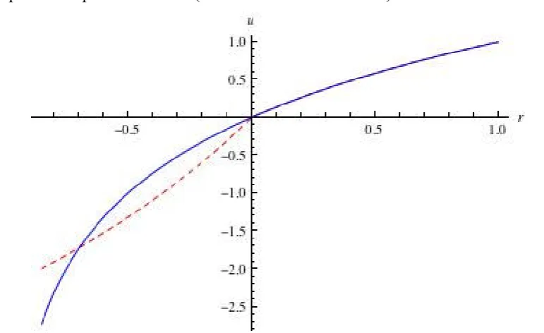
a) The perception utility is generally described by a logarithmic function, which is steeper for

losses than for gains (see Figure 5.1); this utility specifically applies to cases where gains ap!

pear in the problem context (either with or without losses).

Figure 5.1 Logarithmic perception utility function (blue). A convex utility for losses (dashed red) is the “re6

flected” part for gains and applies only in the absence of gains.

b) The perception utility is, however, “reflected” when gains do not appear in the problem con!

text; in this case people invert losses into “gains”, then assess them by the “right!hand” (con!

cave and less steep) part of the logarithmic utility function, and afterwards invert the result

once again to the loss domain; this process gives the impression that the utility function is

claims). The basic explanation for this “reflection” is that positive numbers are easier to oper!

ate than negative ones. Similarly, many people prefer to use their right hand; however moving

a task to the right hand is only possible when it is not occupied with another task.

According to the hypothesis presented here, the logarithmic perception of losses and gains

is the default process and any “reflection” of the perception utility curve for losses is merely an

exception to the rule. The are several arguments to support this claim.

First, while most people are risk seeking towards losses, a considerable minority are risk

averse. This suggests that this latter group perceives losses logarithmically, i.e. it does not “re!

flect” perception utility, even when gains are absent. This perception “misorder” not only ex!

plains the diverging risk attitudes evinced by different subjects, but also the diverging risk atti!

tudes evinced by the same person for different magnitudes of loss.

Second, any perception utility “reflection” disappears under time constraints. This was ex!

amined by Kocher et al. (2011): “In the baseline condition with no time pressure, our data show

the common pattern of ‘partial reflection’. There is strong risk aversion for gains, but mild and

insignificant risk seeking for losses. Under time pressure, we obtain risk aversion for both gains

and losses, i.e. risk seeking for losses without time pressure turns into risk aversion for losses

under time pressure”. This pattern seems obvious as the additional brain operations that “reflec!

tion” require take time. Under time pressure, people revert to their basic instincts.

Third, the described mechanism finds confirmation in brain activity research. Smith et al.

(2002) report that their results “suggest two disparate, but functionally integrated, choice systems

with sensitivity to loss: a neocortical dorsomedial system related to loss processing when evalu

ating risky gambles, and a more primitive ventromedial system related to processing of other

stimuli. This anatomy suggests that choice under loss generates more use of the calculational

part of the brain and diminishes the role of visceral representations in the ventromedial system

which appear to be present under the other conditions”. The hypothesis thus explains the differ!

ent conclusions regarding brain activity. Losses examined separately invoke a more complex sys!

tem, which requires more calculation power. In all other cases (including mixed lotteries like in

Tom et al., 2007) only the basic system is active.

Fourth, utility “reflection” disappears when gains are present in the context of losses. This

ple compare gains and losses and assess them on a common scale”. In this case, the perception

utility function is logarithmic over the whole domain. “When gains and losses are not context for

each other the asymmetry fails to appear”. In this case, utility for losses is often “reflected”, and

is similar in shape and magnitude to that for gains.

Fifth, the hypothesis easily explains the gain!loss separabiliy violations discussed in the

next Point.

6

Gain6Loss Separability Violations

Wu and Markle (2007) consider several cases in which gain!loss separability is violated.

Let us analyze one such case (No. 6 in Table 1 in their paper). The following two choices are

considered, one concerning gain prospects, the other loss prospects.

Problem 1 (Gain Prospects):

H+: $750 with a probability of 0.40 or $0 otherwise [26.4%]

L+: $500 with a probability of 0.60 or $0 otherwise [73.6%]

Most participants prefer lottery L+ (choices are presented in brackets).

Problem 2 (Loss Prospects):

H!: !$1000 with a probability of 0.60 or $0 otherwise [25.0%]

L!: !$1500 with a probability of 0.40 or $0 otherwise [75.0%]

Most participants prefer L!. The above gain and loss prospects are then composed into mixed

prospects.

Problem 3 (Mixed Prospects):

H: $750 with a probability of 0.40 and !$1000 with a probability of 0.60 [51.4%]

L: $500 with a probability of 0.60 and !$1500 with a probability of 0.40 [48.6%]

A slight majority of participants prefers H to L in this case. These results violate gain!loss

separability, which requires that mixed lottery H be preferred to mixed lottery L if the gain por!

tion of H is preferred to the gain portion of L and the loss portion of H is preferred to the loss

portion of L.

Wu and Markle try to explain this violation on the basis of probability weighting. The so!

lution has, however, some drawbacks: “Contrary to most previous studies, the (curvature) pa

rameter for losses was substantially lower than for gains, but most critically, the parameter cap

tive, indicating a more curved weighting function for mixed gambles than for single domain

gambles”. The authors go on to argue that “the observed choice patterns are consistent with a

process in which individuals are less sensitive to probability differences when choosing among

mixed gambles than when choosing among either gain or loss gambles”. If true, this would be a

completely new and hitherto unreported property of probability weighting. The authors also offer

“an alternative explanation for our observed violations of gain loss separability that participants

may be using an ‘extreme outcome heuristic’”. However, “this heuristic, while interesting,

clearly has less generality than our explanation in terms of diminished sensitivity to probabili

ties”.

This change in preference can, however, be easily explained using the hypothesis pre!

sented here. This is done by applying the expected utility formulation without any recourse to the

probability weighting. In Problem 1, the following condition has to be satisfied:

(

)

(

)

u >u (6.1)

As the expected value of both prospects is the same (+$300), the explanation of this pat!

tern only relies on marginal utility diminishing as gain outcomes increase. This is equivalent to

the concavity of the utility curve for gains. In problem 2, the following condition has to be satis!

fied:

(

)

(

)

u − <u − (6.2)

As the expected value of both prospects is likewise the same (!$600), the explanation of

this pattern only relies on the marginal disutility diminishing as loss outcomes increase. This is

equivalent to the convexity of the utility curve for losses, which demonstrates the utility “reflec!

tion”.

In problem 3, which is the composition of Problems 1 and 2, the gain portion of H is not

as good as the gain portion of L, as presented in Problem 1. The explanation of Problem 3 (that H

is anyhow preferred over L) would thus require the loss portion of H to be much better than the

loss portion of L:

(

)

(

)

u − >>u − (6.3)

where “>>” denotes “much more”. This requirement is in strong contradiction with the one de!

manded in Problem 2 (6.2). It requires that utility diminishes quickly as loss outcomes increase,

i.e. to be a steep and concave function. This is exactly what the logarithmic function looks like.

rithmic perception utility function holds over the whole outcome domain when gains are present

in the problem context. The “reflected” utility only appeared in Problem 2, where gains were not

considered.

Please note that the main impact on this paradox has a negative outcome of !1500. In

Problem 2, where utility for losses is convex due to “reflection”, this outcome does not “look” all

that bad when compared with an outcome of !1000; therefore it is preferred once respective

chances are taken into consideration. However in Problem 3, where utility is logarithmic, this

outcome is much worse than an outcome of !1000 and makes the whole prospect (including its

more attractive gains) seem inferior. This shows why and how Wu and Markle could come to an

‘extreme outcome heuristic’ as a possible explanation of the violation.

This example shows that the recently reported “paradoxes” result from taking convex util!

ity for losses as the rule. The gain!loss separability is indeed violated but this fact finds an easy

explanation once convex utility for losses is only assumed in the exceptional case where gains do

not appear in the problem context.

It is interesting to note that Birnbaum (2007), who analyzed the same violation, came to

essentially the same solution: “Gambles with strictly nonpositive consequences are calculated by

substituting absolute values for the consequences in (the general TAX formula) using the same

parameters and multiplying the resulting positive utility by −1. This assumption implies the

“reflection” property”. On the other hand “mixed gambles, as well as gambles composed of

strictly nonnegative consequences, are both calculated by substituting algebraic values into the

(general TAX formula)”. Birnbaum’s reasoning is based on his TAX theory so it differs in many

other details. Most significantly, Birnbaum assumes a linear utility function for both gains and

losses, and explains changes in risk attitudes by a probability weighting mechanism; more spe!

cifically by a transfer of weights from higher to lower lottery branches. The essence of his solu!

tion, however, is that loss prospects are calculated differently than gain and mixed ones, and that

this calculation assumes a double transformation of losses into gains and back into the losses.

This is also the essence of the hypothesis presented here.

7

Discussion

Prospect and Cumulative Prospect Theory define the following characteristics of the value

aversion is modeled using a coefficient λ, and gains and losses are evaluated separately using re!

spective value and probability functions.

In view of recent experimental results, these postulates cannot be held any longer. This

paper presents a hypothesis which asserts that perception utility is generally logarithmic in shape

both for gains and losses. Any “reflection” of the utility curve for losses is merely an exception to

the rule. Several arguments confirming this statement have been presented. The hypothesis easily

explains gain!loss separability violations and leads to a different evaluation of mixed prospects

than that postulated by Cumulative Prospect Theory. Loss aversion is simply a result of applying

a logarithmic function to both gains and losses.

Most significantly, the hypothesis presented here establishes a link between psychological

experiments and financial applications. The latter often consider the compromise between ex!

pected returns and risks offered by prospects (usually mixed ones). These considerations are

founded on Portfolio Theory (Markowitz, 1952A), the basic theory of financial markets. This the!

ory used the property that if the utility function is locally approximated by the quadratic function,

then the prospect expected utility value can be approximated by a function depending on mean

and variance only. The former represents the expected return, the latter the risk associated with it.

Very obviously the logarithmic function proposed by the present hypothesis can be well ap!

proximated around 0 using the quadratic function for a wide range of positive and negative out!

comes (the logarithmic function was considered by Markowitz himself). This is not the case with

the Prospect Theory value function which not only presents a kink at the origin but also changes

its curvature from convex to concave there. The shape of the value function thus breaks all possi!

ble connections between Prospect Theory and Portfolio Theory. This paper shows, however, that

the shape of the value function proposed by Prospect Theory is incorrect (at least for mixed pros!

pects) and that the perception utility function conforms the basic Portfolio Theory assumption.

This opens the way for an integrated psycho!financial theory of behavior – something not possi!

ble under the Prospect Theory paradigm.

This raises the question whether perception utility is able to explain all the behavioral

paradoxes considered by Prospect Theory. The answer is negative because it only represents the

bottom layer of a decision making model. Decision Utility Theory (Kontek, 2010, 2009), which

offers an alternative solution to Cumulative Prospect Theory, distinguishes between perception

monetary outcomes, are perceived. The hypothesis regarding the shape of this utility has been

presented in this paper. Per contra, decision utility describes how these perceived and framed out!

comes are treated when taking risky decisions. It has to be pointed out that the term “decision

utility” introduced by Kontek is a very different concept from “decision utility” introduced re!

cently by Kahneman (1999). The latter is just another name for the value function. Kontek’s the!

ory postulates a double S!shaped decision utility curve similar to the one hypothesized by

Markowitz (1952B), and applies the expected decision utility value similarly to the theory by von

Neumann and Morgenstern (1944). Perception utility, framing, and decision utility are thus the

three layers of a multi!layer decision making model (Kontek, 2010, 2009). Interestingly, this so!

lution does not require the probability weighting concept to explain behavioral paradoxes.

References:

Abdellaoui, M., Bleichrodt, H., Parashiv, C., (2007). Loss Aversion under Prospect Theory: A Parameter!Free Measurement. Management Science, 53(10), pp. 1659!1674.

Abdellaoui, M., Bleichrodt, H., Haridon, O. L., (2008). A Tractable Method to Measure Utility and Loss Aver! sion under Prospect Theory. Journal of Risk and Uncertainty, 36(3), pp. 245!266.

Birnbaum, M. H., Bahra, J. P., (2007). Gain!Loss Separability and Coalescing in Risky Decision Making. Management Science, 53, pp. 1016!1028.

Blavatsky, P. (2005). Back to the St. Petersburg Paradox?, Management Science 51, pp. 677!678.

Booij, A. S. G., van de Kuilen, (2006). A parameter!free analysis of the utility of money for the general popula! tion under prospect theory. Working Paper, University of Amsterdam.

Etchart!Vincent, N., (2009). The shape of the utility function under risk in the loss domain and the ‘ruinous losses’ hypothesis: Some experimental results. Economic Bulletin, 29(2), pp. 1404!1413.

Fehr!Duda, H., de Gennaro, M., Schubert, R., (2006). Gender, Financial Risk, and Probability Weights. Theory and Decision, 60, pp. 283!313.

Gonzales, R., Wu, G., (1999). On the Shape of the Probability Weighting Function, Cognitive Psychology, 38, pp 129!166.

Kahneman, D., Tversky, A., (1979). Prospect theory: An analysis of decisions under risk. Econometrica, 47, pp 313!327

Kahneman, D., Knetsch, J., Thaler, R., (1990). Experimental Test of the endowment effect and the Coase Theo! rem. Journal of Political Economy 98(6), 1325!1348.

Kahneman, D. (1999). Objective Happiness. In Kahneman, D., Diener, E. Schwarz, N. (Editors) Well Being. The Foundations of Hedonic Psychology. Russell Sage Foundation. pp. 302!329.

Kocher, M., Pahlke, J., Trautmann, S., (2011). Tempus Fugit: Time Pressure in Risky Decisions. Munich Dis! cussion Paper No. 2011!8, Department of Economics, University of Munich, http://epub.ub.uni! muenchen.de/12221/

Kontek, K. (2010). Decision Utility Theory: Back to von Neumann, Morgenstern, and Markowitz. Working Pa! per available at: http://ssrn.com/abstract=1718424

van de Kuilen, G., (2007). The economic measurement of psychological risk attitudes. Dissertation, Faculty of Economics and Business, University of Amsterdam. http://dare.uva.nl/document/44755

Lattimore, P. K., Baker, J. R., Witte, A. D., (1992). The influence of probability on risky choice: A parametric examination. Journal of Economic Behavior and Organization, 17, pp. 337!400.

Libby, R., Fishburn, P., (1977). Behavioral Models of Risk!Taking in Busieness Decisions: A Survey and Evaluation. Jornal of Accounting Research, 15(2), pp. 272!292.

Litt, A., Eliasmith, C., Thagard, P., (2008). Neural affective decision theory: Choices, brains, and emotions. Cognitive Systems Research, 9, pp. 252!273.

Markowitz H., (1952A). Portfolio Selection, Journal of Finance, 7(1), 77!91.

Markowitz H., (1952B). The Utility of Wealth. Journal of Political Economy, Vol. 60, pp. 151!158.

McGraw, A. P., Larsen, J. T., Kahneman, D., Schkade, D., (2010). Comparing Gains and Losses. Psychological Science, 21(10), pp. 1438!1445.

Neilson, W. S, Stowe, J., (2002). A Further Examination of Cumulative Prospect Theory Parameteriza! tions. Journal of Risk and Uncertainty, Springer, vol. 24(1), pages 31!46, January

von Neumann, J., Morgenstern, O., (1944). Theory of Games and Economic Behavior, Princeton University Press.

Payne, J. W., Laughhunn, D. J., Crum, R., (1980). Translation of gambles and aspiration level effects in risky choice behavior. Management Science, 26, pp. 1039!1060.

Pennings, J. M. E., Smidts, A., (2000). Assesing the construct validity of risk attitude. Management Science, 46, pp. 1337!1348.

Prelec, Drazen. (1998). The Probability Weighting Function. Econometrica, 66:3 (May), 497!527.

Scholten, M., Read, D., (2011). Anomalies to Markowitz’s Hypothesis and a Prospect!Theoretical Interpreta! tion. SSRN Working paper: http://ssrn.com/abstract=1504630

Smith, K., Dickhaut, J., McCabe, K., Pardo, J. V., (2002). Neuronal Substrates for Choice Under Ambiguity, Risk, Gains, and Losses. Management Science, 48(6), pp. 711!718.

Stevens, S. S., (1957). On the psychophysical law. Psychological Review 64(3), pp. 153–181.

Tom, S. M., Fox, C. R., Trepel, C., Poldrack, R. A., (2007). The Neural Basis of Loss Aversion in Decision! Making Under Risk, Science, 315, pp. 515!518.

Tversky, A., Kahneman, D., (1991). Loss Aversion in Riskless Choice: A Reference!Dependent Model. The Quarterly Journal of Economics, 106(4), pp. 1039!1061.

Tversky, A., Kahneman, D., (1992). Advances in Prospect Theory: Cumulative Representation of Uncer! tainty. Journal of Risk and Uncertainty, Springer, vol. 5(4), pp 297!323.

Wu, G., Markle, A. B., (2008), An Empirical Test of Gain!Loss Separability in Prospect Theory. Management Science, 54, pp. 1322!1335.