CONDOR 3 A Two Dimensional Reactor Lifetime Program with Local and Spectrum Dependent Depletion EUR 4539

mm

im

M»

■¡Ml

■MSHHiíffil ¡i&ï

THE EUROPEAN COMMUNITIES

« «tiliUîll»

«8

«c«

I »il

l ¡

I f l É K i

CONDOR 3

Ι Ι Ρ Κ

A TWO­DIMENSIONAL R E A C T O r a l I ! «

TÍ

LIFETIME PROGRAM WITH LOCAL ANM

>ECTRUM DEPENDENT DEPLETION |

|

Iwl

h

WÊÊm

f

m

*a

m

«li

teag

'< T i . I

ffl\

mi

m

vìi

ff-Contract EURATOM/FIAT/A.R.S. No. 089­66­2 TEEI

lili

peiiiiiiliïililiii

&w3

JilWï!

This document was prepared under the sponsorship of the Commission of the European Communities.

Neither the Commission of the European Communities, its contractors nor any person acting on their behalf :

Make any warranty or representation, express or implied, with respect to the accuracy, completeness, or usefulness of the information contained in this document, or that the use of any information, apparatus, method, or process disclosed in this document may not infringe privately owned rights : or

EUR 4539 e

CONDOR 3 — A TWO­DIMENSIONAL REACTOR L I F E T I M E PROGRAM WITH LOCAL AND SPECTRUM D E P E N D E N T DEPLETION by E. SALINA (A.R.S.)

Commission of the European Communities Report prepared by A.R.S., S.p.A.

Applicazioni e Ricerche scientifiche, Milan (Italy) Contract EURATOM/FIAT/A.R.S. No. 089­66­2 T E E I Luxembourg, November 1970 ■— 82 Pages — BF 125.—

CONDOR 3, as the preceding nuclear codes of the CONDOR series is a few­group bidimensional lifetime program written in Fortran IV for the IBM 360/65. It couples the method of the spatial modal expan­ sion with the 5 point finite difference method.

By means of the spatial modal expansion the program determines the eigenvalue of the reactor, which can be in turn the Kl f t (multi­

plication factor), the (H) (dilution factor of a diluted poison), the 2P or

the boundary of a prefixed control region.

By means of the finite difference method, the program improves the calculation of the Kof( and the group flux spatial distribution.

EUR 4539 e

CONDOR 3 — A TWO­DIMENSIONAL REACTOR L I F E T I M E PROGRAM WITH LOCAL AND SPECTRUM D E P E N D E N T DEPLETION by E. SALINA (A.R.S.)

Commission of the European Communities Report prepared by A.R.S., S.p.A.

Applicazioni e Ricerche scientifiche, Milan (Italy) Contract EURATOM/FIAT/A.R.S. No. 089­66­2 T E E I Luxembourg, November 1970 — 82 Pages — BF 125.—

CONDOR 3, as the preceding nuclear codes of the CONDOR series is a few­group bidimensional lifetime program written in Fortran IV for the IBM 360/65. It couples the method of the spatial modal expan­ sion with the 5 point finite difference method.

By means of the spatial modal expansion the program determines the eigenvalue of the reactor, which can be in turn the Ketf (multi­

plication factor), the (H) (dilution factor of a diluted poison), the Σν or

the boundary of a prefixed control region.

By means of the finite difference method, the program improves the calculation of the K„rr and the group flux spatial distribution.

EUR 4539 e

CONDOR 3 — A TWO­DIMENSIONAL REACTOR L I F E T I M E PROGRAM WITH LOCAL AND SPECTRUM D E P E N D E N T DEPLETION by E. SALINA (A.R.S.)

Commission of the European Communities Report prepared by A.R.S., S.p.A.

Applicazioni e Ricerche scientifiche, Milan (Italy) Contract EURATOM/FIAT/A.R.S. No. 089­66­2 T E E I Luxembourg, November 1970 — 82 Pages — BF 125.—

CONDOR 3, as the preceding nuclear codes of the CONDOR series is a few­group bidimensional lifetime program written in Fortran IV for the IBM 360/65. It couples the method of the spatial modal expan­ sion with the 5 point finite difference method.

By means of the spatial modal expansion the program determines the eigenvalue of the reactor, which can be in turn the Kerr (multi­

plication factor), the (H) (dilution factor cf a diluted poison), the Σν or

the boundary of a prefixed control region.

EUR4539e

COMMISSION OF THE EUROPEAN COMMUNITIES

C O N D O R 3

A TWO-DIMENSIONAL REACTOR

LIFETIME PROGRAM WITH LOCAL AND

SPECTRUM DEPENDENT DEPLETION

by

E. SALINA (A.R.S.)

1970

Report prepared by A. R. S., S.p.A.

ABSTRACT

CONDOR 3, as the preceding nuclear codes of the CONDOR series is a few-group bidimensional lifetime program written in Fortran IV for the IBM 360/65. It couples the method of the spatial modal expan-sion with the 5 point finite difference method.

By means of the spatial modal expansion the program determines the eigenvalue of the reactor, which can be in turn the Keff

(multi-plication factor), the (H) (dilution factor of a diluted poison), the 2P or

the boundary of a prefixed control region.

By means of the finite difference method, the program improves the calculation of the Keff and the group flux spatial distribution.

KEYWORDS

MATHEMATICS COMPUTERS FORTRAN IBM 360 REACTORS NUMERICALS POISONING

INDEX Pag.

INTRODUCTION and SUMMARY 5

I THE DIFFUSION EQUATIONS 11 II GENERAL FEATURES OF THE PROGRAM 17

III SELF-SHIELDING FACTORS AND MACROSCOPIC CROSS-SEC

TIONS 24 IV DEPLETION EQUATIONS 26

V PROGRAM OUTPUT 30 VI PROGRAMMED STOPS 31

VII UNIT SYSTEM 32 VIII PROGRAM ORGANIZATION 32

IX INPUT DATA PREPARATION 34 X INPUT DATA FOR RESTART 62

XI HOW TO SAVE THE FLUXES 65 XII HOW TO SAVE THE DATA FOR RESTART 66

XIII HOW TO SPECIFY PCINT FLUXES AND NUMBER DENSITIES

BY MESH-ELEMENT 67

XIV HOW TO MAKE A RESTART 68

APPENDIX A - Computational Restrictions in the Solu­

tions of the Depletion Equations 69 APPENDIX Β - Peripheral Unit Configuration 71

APPENDIX C - Program Restrictions 72

REFERENCES 73 ACKNOWLEDGEMENTS 74

5

-INTRODUCTION AND SUMMARY *)

CONDOR-3, as the preceding nuclear codes of the CONDOR series (5,l4), is a few-group bidimensional lifetime program written in Fortran IV for the IBM 36O/65. It couples the method of the spatial modal expansion (3,9,11) with the 5 point finite difference method.

By means of the spatial modal expansion the program determines the eigenvalue of the reactor, which can be in turn the K f f

(multiplication factor), the Θ (dilution factor of a diluted poison), the 2 or the boundary of a prefixed control region.

By means of the finite difference method, the program improves the calculation of the K(off and the group flux spatial distri­

bution.

The coupling between the two methods has been suggested by the realization that the spatial modal expansion is able to deter­ mine the eigenvalue of the reactor with an acceptable precision,

even in reactors where the point fluxes, especially the thermal ones, disagree to a large extent with the point fluxes deter­ mined by means of the finite difference (4).

The main advantages attainable in using the CONDOR programs are:

1) The criticality searches are very speedy, for they are per­ formed by the modal expansion only.

2) The modal expansion fluxes can be used as initial guess for the finite difference calculations.

Due to advantages 1), 2) and referring to a many point calcu­ lation (> - 4000 points), one can state that the computational time required for a diluted poison search (with final finite difference calculation) is nearly the came as that required for a straight K-effective calculation with a flat guess for the finite difference fluxes.

J>) A problem can be restarted from any time-step already car­ ried out, using basically a tape ana cards only for those data which are to be changed.

6

-The main features of C0ND0R-3 which are not present in C0ND0R-2, are:

1) The depletion equations are solved at eaeh mesh element (i.d. the reetangular cell bounded by two suceessive horizontal and vertical mesh lines) and so the fuel burn-up calculation is as refined as possible, while in C0ND0R-2 it was carried out only regionwise, a region being a collection of mesh-rectangles.

2) More than one cross-section library can be specified by cards and therefore the microscopie cross-sections may have diffe-rent values in diffediffe-rent regions.

3) As an alternative to the straight specification by cards (as explained above), the microscopic cross-sections can be cal-culated at each time-step by the program itself, taking into account the local values of some basic parameters such as'the moderating ratio, the Pu-concentration, the fuel and

modera-tor temperatures ete.

Details about the actual computational procedure which ob-viously must be set up bearing in mind the reactor type (6), can be found in Appendix E.

A brief aceount of the main physical features of the program is summarized.

Depletion Equations

7

-Number of groups

The program performs optionally from 1 to 4 group calculations.

Types of poisons:

There are 4 types of poisons:

a) The burnable poisons. They are treated in the depletion equa­ tions.

b) A uniform poison smeared over the entire reactor; because it simulates a chemical poison, it will be called diluted pol-son from now forth.

Its absorption cross-section in group i is the product of a 2, , a group fraction t, and a dilution factor. Θ . This last

factor can be varied to maintain the criticality.

c) A number of poisoned regions, called rodded regions, because they simulate banks or rings of homogenized control rods, each characterized by a 2 (different from one region to another). The rodded regions can be defined independently and superposed on the reactor regions, about which we shall talk later on

(see Region and Composition). The criticality can be maintained managing the rodded regions, either varying the boundary or

the value of Σ (see Diffusion calculations), _rp

v

d.) The so-called non-diffusion regions (rod regions) where the fluxes of one or more groups are not calculated but satisfy, on the boundary, to a logarithmic derivative condition of the form

^ i 3 Φ 1 Λ ϋ

3n 2 — „ _ c φ i =» group index

3 _{derivative normal to region}

boundary and C1A" is a given positive constant. an

Diffusion Calculations

At each time step the program may perform optionally 4 types of diffusion calculations:

i) straight K-effec'tive calculation;

li) criticality calculation, varying the dilution factor ø(cfr. Types of poisons, point b)) until a given Κ ^ is reached.

This option simulates the control by means of a chemical

- 8

iii) critioality calculation, varying the top boundary of a spe­ cified rodded region or group of rodded regions. If the top or bottom limit of the moving boundary is achieved without reaching the criticality, the program goes to the next rodded region or group of rodded regions, specified by a list (cfr. Control Programming);

iv) same as iii) but the varying parameter is the 2 instead of the boundary.

Control Programming

A list of "rodded regions" can be specified at the beginning of life. The criticality then will be maintained during the burn-up of the reactor by managing the 2 or the boundary in one region at the time (or in one group of regions), following the specifi­ cation list. Once the poison of a "rodded region" is totally re­ moved (or removed up to some prefixed value) the program auto­

matically goes on to adjust the poison ih the next region or group of regions specified in the list.

Cross-section Library

Each cross-section library is divided into 3 main blocks:

block A: library of microscopic cross-seetions Q. (transport), n. (absorption), σ,, (removal to next group) for any iso-_{a ι} tope;

block B: library of microscopic cross-sections of(fission), v of

(nu-fission), e (energy per fission) for any fissionable isotope;

block C: fission yields for any fissionable isotope.

At any time step the program can read in any or all of the blocks A, B, C. A block may be read only partially for a restricted num­ ber of elements.

­ 9 ­

Self­Shielding Factors

The isotopes can be assigned either constant self­shielding faotors or self­shielding factors which are concentration­depen­ dent with a polynomial law:

ρ « mesh element index ç*'J'P ­ f a*"1'1 ( NJ'p)h i ­ group index

J =» isotope index

1 « index of the region of which element ρ is a part

ci*J,Ρ m self­shielding factor

Ν*''*' » number density in mesh element ρ

The self­shielding factors and (or) the polynomial coefficients may be read in at any time­step.

Time­step Data

First, we shall define what is meant exactly as a "time­step". A time­step begins with the calculation of the new number densi­ ties (burn­up calculation) and ends with the calculation and the normalization of the group fluxes (diffusion calculation). Excep­ tion is made for the time­step 0, where the burn­up calculation is replaced by the mere specification of the input number densi­ ties.

The duration and the reactor power at each time­step can be arbi­ trarily prefixed. Moreover, each time­step can be divided at will into a number of smaller substeps of the same length.

At each time­step the program carries out only one diffusion cal­ culation while at each substep it recalculates the concentration­ dependent self­shielding factors and the time­dependent number densities with no flux renormalization taking place.

10

-owing to machine error, time overflow, etc., can be restarted. If the interruption is programmed to occur in a restart point, as it is possible to the user, there is no loss of computer time.

time-step 0 time-step 1 time-step 2 time-step k

B.C. = burn-up calculation N.D. » new input data

Sii. « shuffling

D.C. = diffusion calculation R.P. « restart point

fig. 1

Region and Composition

It is easy to realize that, after the first time-step has elap-sed, each mesh rectangle (or mesh element) has a different com-position, owing to the spatial distribution of the fluxes. Never-theless more mesh elements may be arranged into the same region. A region is defined as a collection of one or more mesh elements, even disjoint, which have the same buckling, the same diluted poison cross-section, the same library and self-shielding data and the same initial composition. The idea of region is introdu-ced especially for input purposes in order to make the specifica-tion of the input data easier, but it may be even physically meaningful, with reference to the initial status of the reactor, since the program calculates and prints integrated quantities and flux weighted macroscopic cross-sections, showing up in this way the total effect of the burn-up at each region.

11

input atomic densities.

Shuffling

At any prefixed time­step the program may take the (time­dependent) number densities of a rectangular block of mesh elements and, af­ ter clockwise or counter­clockwise rotation, transfer them in an­ other rectangular block element by element. For instance, a pos­ sible pattern is sketched in fig. 2.

Also fresh fuel (that is a uniform mixture made up of the isotopes present at the beginning of life) can be fed into any rectangular block of mesh elements. Moreover, a new region index can be assig­ ned to the mesh elements.

The above operations can be repeated for as many rectangular blocks as desired and can be used to simulate the transfer and the sub­ stitution of fuel elements or the replacement of a control rod by its follower.

1

k-7

Å0

ι

6

?

M 3

G

9

U

Jo

M

Ål

■ %

î

3

k-5 6

Λ

a

3

■ '■ - ■ ■ - ■

ι ι

ι

1st block rotation

(90 clockwise)

translation 2nd block

fifi­ 2

I ­ THE DIFFUSION EQUATIONS

I.1 ­ Statement of the Problem

At any time­step, the stationary group diffusion equations are (the time­step index having been dropped):

­ divf D1(x,y)grad ®i(x,y)] + [2T(x,y) +2p(x,y)] 9i(x,y) »

jL n g i|fi(x,y)

*1(x,y) ­ *­ Y v2fJ(x,y)9J(x>y) +2^~1(x,y)<Pi"1(x,y)

12

1,2, ... ng

The physical interpretations of these symbols are:

i « group index;

ng » number of groups (ng < 4 ) ;

2

R « °

4 «

2

a - 4

+ ß J B

i

4 - K

2

dp * <*

2

r

P

2a ■ the macroscopic absorption cross­section

a

2R β the macroscopic removal cross­section

ρ

B, » the transverse buckling

D « the diffusion coefficient

2, » the macroscopic absorption cross­section of a diluted poison (dp)

t. « fraction of 2* in the group i

Ô « dilution fraction. It may be either an eigenvalue of the problem, or an input data

2 «■ the macroscopic cross­section of a rodded poison (rp) Also 2 may be either a problem eigenvalue or a given data

tì = fraction of 2_ in the group i

r. rp

v2f » the macroscopic cross­section of neutron production

φ ­ the neutron flux

χ » the fission spectrum integral over group 1

13

Any equation of system (1­1) must be solved at each point inter­ nal to the domain R, delimited by the external contour I of the

reactor.

i i i —

The functions φ (χ,y) and ψ (x,y) on I f u l f i l l the boundary con­

ditions of the type:

(p

1

(Xiy) ­ / ( x , y ) ·» 0

a n

a n

w

(1­2)

. (x,y) 3 Γ

The domain R is also delimited internally by one or more internal contours γ. , on which the flux φ (x,y) fulfills the condition of assigned logarithmic derivative of the type:

DÌ<x'y> i r ! * 01(χβγ)φί = 0

(x,y)3

Yn

(i-J)

where C is a positive function.

The internal contours γ, are the contours of the non-diffusion regions, where the flux <p of one or more groups, but not neces­ sarily of all, is not defined in the points inside.

Moreover, the functions φ (χ,y) and D (x,y) . grad φ (χ,y) are to be continuous in any point of the domain R.

1.2 - Solution of the Problem by Means of the Spatial Modal ßxpan· sion and Variational Technique

If the functions ψ (x,y) are supposed known, then the functions φ (x,y) that satisfy eqs. (1­1), conditions (1­2), (1­3)* and the

14

-Ρ*[ φ

1

(χ,Υ) 3 ­ / Γ Ι

DÌ

(

x

*y) grad φ

1

. grad φ

1

+ |[2*(x,y) +

+ 2^(x,y)] .[ 9i(x,y)]2 ­ti(x*y) «(x,y) 1 P ( X ) ¿χ dy +

+ Σ Φ | c1( x . y ) [ç i( x , y ) ]2 d o (1­4)

h­i rn

where the symbol . represents the scalar product, η, is the num­ ber of logarithmic regions, and:

(x) . « 2 %x in cylindrical geometry ­> lj. in plane cartesian geometry

l·,

The symbol (¡) represents an integral over an internal contour,

Yh

and it is a curvilinear integral in cartesian geometry and a sur­ face integral in cylindrical geometry.

The flux φ (χ,y) is expanded in a series of eigenfunctions : x*'

nx riy

,

i

( x , y ) «

y

y

c¿

k

χν, (χ) Y

k

(y)

(1­5)

where n and n are the number of eigenfunctions taken in direc­

x y

tions χ and y respectively.

n. » n . n is the total number of two­dimensional harmonics

h χ y

whk(x,y) =» xh(x) Yk(y)

The eigenfunctions Xh(x) a n d Yk(y) a r e c h o se n such that they

themselves satisfy the conditions (1­2) on the external boundary. The program CONDOR employs the following eigenfunctionsj

15

-/'cos(2h ­ 1) £*­

■^x

Xh(x)J

s i n h 22,

L

x

( c o s ( 2 k ­ 1)

SL

r

k

(yW

I s i n k

2äL

Ly

both in cylindrical and cartesian geometry, with a symmetry condi­

tion at χ β 0

in cartesian geometry with the oondition φ (χ,y) ( Q = 0

' " (1­6)

cartesian geometry with symmetry condition at y = 0

cartesian geometry with the con­ dition φ (χ,y)

y=0

= 0

(1­7)

L and L are the two sides of the rectangular domain R.

χ y

The program CONDOR does not solve oell problems: the fluxes are always supposed to vanish on the right and bottom contours of the reactors.

The domain R is represented in fig. 3·

m=m ["""contour

internal inter­ faces * contour

fig­

2

1.3 ­ Matricial Form of the Diffusion Equations

By substituting the series expansions (1­5) into the functionals

(1­4), the coefficients of the fluxes ayia are determined by e­

quations (1­9)s

re

3 ar s

0 (r ­ 1,2, ... ηχ; s » 1,2, ... η ; i = I, ... η )

16 ­

Defining:

A

hkrs

β

/

D Ì

(

x

' y ) [

X

h (

x

) V

y

) M

x

> V

y

>

+ x h

(

x

)

Y

k

( y )

M

x )

V

y

^

R

(1­10)

p(x)dxdy +

ƒ[ 2^(x,y) + 2¿(x,y)]x

h

(x)Y

k

(y)x

r

(x)Y

s

(y)p(x) dx dy

*

R (

ι -ii)

S

hkrs

β

ƒ v 4

( x

'

y

)

X

n

( x

) V

y

)

X

r

( x

)

Y

s

( y ) p

(

x ) to dy

^'

U

^

R

R

hkrs - ƒ 4

( x

'

y ) X

h

( x ) Y

k

( y ) X

r

( x ) Y

s

( y ) p ( x ) dx dy (1_12)

R

Equations (1-9) are reduced to the following system of n, linear

i

equations in the n, unknowns a,.:

n

x

n

v i

V \

A

hkrs

a

hk ° 7" ^ s

+

y

R

hkrs

a

hk

nWi Esi h, k

*rs » L Σ

S

hkrs "hk (1-13)

J-l h,k

R

hkrs

1

°

Reducing the four-index matrices to two-index matrices, following

the schemes described in (j5), equations (I-I3) can be written in

a compact matricial form:

f

A

i „1

_ ¿

t + H

i­l a

1

"

1

η λ

φ ­ ¿,

sJ

^

(1

'

l4)

R

0

» 0

i ­ 1,2, ... η

Ο

17

statical standpoint (18) coincides with the eigenvalue lar­ gest in modulus of eqs. (1­14), use is made of the straight power method, whose convergence is guaranteed by the fact that system (1­14) can be reduced easily to the classical form:

Μ ψ « λψ (1­15)

The criticality searches are performed by varying the control parameter and solving system (1­14) each time, until the con­ vergence is reached.

More details about the matrix equations (1­14) and its solution can be found in (5,14).

1.4 ­ Restrictions of the Modal Expansion Method

TÌ3.X

The maximum number of harmonics n' permissible in the program CONDOR has been determined in such a way that the matrices A , S , R of eqs. (1­14), taking into account their symmetry, could be simultaneously stored in the fast memory of the available computer, avoiding the time­expensive use of peripheral storage units in the iterative cycles of the power method.

Even with a high number of harmonics (up to 100). the matrices A can be inverted with rapidity and precision by means of a direct method.

Should n ?a x be greater than "100, not only the intervention of

peripheral units would be necessary at each iteration, but also the substitution of the matrix inversion iterative methods to the direct ones.

II. ­ GENERAL FEATURES OF THE PROGRAM

II.1 ­ Types of Reactor Regions

The domain R representing the reactor, is made up of regions which can be of three types:

i) Diffusion Regions, where all group fluxes are defined and ful­ fill eqs. (1­1) with Ό1(x,y) > 0.

uni-- 18

form initial composition, the same buckling, the same diluted poison section, the same microscopic cross-sections and self-shielding data. On the contrary, after the time-step 0, the macroscopic cross-sections D , Σ„,

i i

2 , v2f 1 η a fuel region have different values at each

mesh rectangle owing to the spatial distribution of the fluxes and the consequent non-uniform burn-up of the fuel. Also the absorption cross-section 2 due to a rodded

poison can take different values in points of a same dif­ fusion region (cfr. Rodded Regions), due to the fact that the rodded regions can be superimposed at will over the diffusion regions.

ii) Non-Diffusion or Logarithmic Regions

The flux of one or more groups is not defined in the points internal to sueh a region, but fulfill a condition of as­ signed logarithmic derivative on the contour γ,

pfory? V f o y )

m

.

c

i

7(x7y)

d n

(x,y) 3

Y l

(2-1)

where η is the inwardly oriented normal toy,. For all other groups, the region is a regular diffusion region. We shall call it preferably a logarithmic region, instead of rod region, as PDQ (1) does, to avoid confusion with the rodded regions described below.

The regions considered in i) and ii) are not necessarily rectangular but may have a boundary of whatever shape, pro­ vided it is composed of horizontal and vertical segments of mesh lines. Moreover, a region (e.g. a non-burnable region or a logarithmic region) can be constituted by two or more disjoint sets of mesh points.

iii) Rodded Regions

- 19

t Σ to the pre-existing group - 1 absorption cross-section at every point covered by a rodded region.

They are called rodded regions because they simulate the poison of control rods, properly homogenized and smeared out over portions of the reactor which generally have not the same contours of the diffusion regions.

II.2 - Mesh Points

In order to solve the finite difference equations, derived from eqs. (1-1), the domain R js discretized in a grid of mesh points. The horizontal and vertical lines, called respectively rows and columns of the grid, are separated by intervals of arbitrary width, but they must be assigned in such a way that the external boundary of domain R and the contours of all the regions, of whatever type, coincide exactly with these lines.

The columns are numbered from left to right and the rows from top to bottom, beginning with 1.

The coordinate axes χ and y lie respectively on the top and left contours of the domain R. The y axis is oriented downwardly. Fig. 4 will show an example of grid.

The rectangular symmetry axes, if any, lie on the coordinate axes. Moreover, there may be a diagonal symmetry axis through the origin (1,1) and oriented to 45 with respect to the coordi­ nate axes.

. Ί 2 3 4 5 6 1 S J Λ0 11

2

4 5

6

Τ

V

f

I

I

iç· 4

>-20

II.5 ­ Diffusion Calculation and Criticality Searches

The diffusion equations (1­1) can be solved in three different ways, depending on what parameter is considered as the eigen­ value of the system (1­1).

1) Straight K f f Calculation. This coincides with the χ greatest

in modulus of eqs. (1­14).

2) Diluted Poison Search. At any time­step the program deter­ mines the critical dilution factor Θ(crit) for a wanted eigenvalue χ with the following procedure:

G

a) The program calculates the eigenvalue χ (=K ff,) f or Θ = Θ

where © (max) iS the maximum allowable dilution factor gi­

ven in input. If x ( ©m a x' ) >X , meaning that the reactor is

supercritical even with the maximum poison concentration, the program stops.

If χ ( ¿max))< λ , the program calculates λ f o r © » © ^

(i ) °

where Θv ; is a guess, supplied by the input for the be­

icrit) ginning diffusion calculation and by the last value © v '

obtained in the preceeding time­step, for the other time­

steps.

b) If χ (©^ ')> X , a new value Θ^ ' is obtained by linear in­ terpolation between Θ ^m ' and ©^ ' .

c) If χ(©^10< Xc, the program evaluates X for © = © ^m n',

where Θ ^m n' is the minimum allowable value of © , given

in input.

If x(©^m ')< x_, meaning that the reactor is subcriticai

even with the minimum poison concentration, the program stops.

d) I? x ( © ^m l nb > Xc> a new value © ^ is obtained by linear

interpolation between ©^ ' and ô^mj­n/.

e) All other values of Θ : Θ ^ ' , ©^ ' ... are obtained by li­ near interpolation between the two last values calculated:

e

( t )

· > " ■ "

*

X

( t ­ i

(

r ! t ­ a j Ιβ<*­

ι

>­β<*­*)]

(2­2)

Χ "λ feriti

21

-2) Rodded Poison Search. As already said, the rodded poison is

present as an absorption 2 in rectangular regions called

rodded regions. The program determines either the critical

feriti fxi

cross-section Σ,ν, '

;

or the critical top

v

'

boundary

fcrit)

y

K

'

of a rodded region for a wanted eigenvalue χ .

c

In both cases, naming V the parameter to determine, the itera­

tive process is based on the following concepts:

a) For each rodded region are specified in input:

- a value of the parameter V

- a value V^

m

', corresponding to a maximum poisoning

- a value V^ ', corresponding to a minimum poisoning.

If the parameter V means the boundary, v^

m i n

^ and v^

m a x

^

are respectively the lower and upper ordinate of the rod­

ded region.

b) The control rods are inserted from bottom to top

v

', that

is the moving boundary advances in the negative sense of

the y axis.

o) A Control List is given in input, that is the sequence of

the rodded regions followed by the program in the critica­

lity searches of this type. A region cannot be repeated

in the list. Two cr more regions listed consecutively in

the control list can be grouped in the same "control bank"

provided that they have the same input values of V^ '

and v^

m a x

'. The program does adjust the parameter V simul­

taneously in all regions belonging to the same control bank.

The first objective of the search is to identify the rodded

bank where the criticality can be reached, that is the bank

in which the parameter V can take a value such that the K

eff

.

is xo.

00

This corresponds to a physical insertion from top to bottom,

­ 22 ­

d) At time­step 0, the program evaluates the Κ r

~

putting

v β

ν"™».,

i n

all rodded regions of the Control List. If

max

Κ

r r

is >X_, the program stops; if Κ

re

<λ , the para­

meter V takes its actual value, specified in input, in

all of the rodded regions, and the program initiates the

search in the first bank of the Control List as explained

in f ) .

e) At the successive time­steps, the program starts the cri­

ticality search beginning with the critical bank of the

preceding time­step.

f) When the program acts on the parameter V of a bank given

in the Control List, primarily calculates the K f

f

for

V « v (

m a x

) . If X ( v (

m a x

) > X , the program leases this

bank with a status of poison specified in g) and goes to

the next bank.

If x(v(

raax

))< x

c

,

the

program calculates X

(V^

min

^)i

if

this is <

\

, the program leaves and goes to the next bank.

If x ( v (

m i n

) ) > x

c

, this means that in this bank the criti­

cality can be attained varying V between V^

m n

' and \ p

m a x

' ,

and this is accomplished by successive linear interpola­

tions, as described in h ) .

g) When the program jumps from one bank to the next as indi­

cated by the Control List, there are two alternatives about

the value taken by the parameter V in the regions of the

just abandoned bank:

1. Parameter V takes its actual input value,

2. Parameter V maintains its last assumed value, that is

v

(max)

l f t h e

^(max))

w a s o r v

(rnin)

l f ( v

( m i n )

}

\äff v»

>

""" '*c ^

v

""

Jv

eff

<*c'

It will be referred to these two alternatives as to the al­

ternatives A and B respectively.

h) When the critical rodded bank is identified (K

f f

(v^

rnax

) )<x

and K

f

,

f

>(V^

ra

)>x „ contemporaneously), the program sear­

ches for the ν

(

·

0Γ1ν/

·' interpolating between the two last va­

23

V^ ' and V^ 't and successively:

v

fc

-v^)

+

tC/zL)

(v^'-v^))

Ke f f ' Ke f f

until a v (c r i t) is found such that:

Ke f f ( V < « » > ) ­ χ , | < η (2­3)

l) If the search is performed following the alternative B, the program stops when all banks of the Control List are exhausted.

On the contrary, when the Control List is exhausted in searches following the alternative A, the program goes back to the first bank of the List and restarts the con­ trol search with the alternative B.

All of the three different diffusion calculations des­ cribed above (Straight K f f, Dilute poison search, Rodded

poison search) are performed by CONDOR by means of the modal expansion method.

Successively, the program evaluates the Κ ^ and the point­ wise group fluxes by means of the finite differences. In the criticality searches (Dilute Poison search, Rodded Poison search), the critical parameter V*· ' found by the harmonics is not revaluated by the finite differences.

The flux guess for the finite differences is supplied by

the flux expansion (2­4):

nx

%

9i

(x,y) =

y y

«¿ie ν * ) Y

k

(y)

(2-

4

)

24

upper boundary

rodded region

lower boundary

III. - SELF-SHIELDING FACTORS AND MACROSCOPIC CROSS-SECTIONS

As already stated, the self-shielding factors ς 'J , p may be

time-independent during the reactor lifetime or may vary with a polynomial law of the form:

6r

ri,J,P = γ* ai,j,l (NJ>P)h

Ν

i » group index

J « isotope index (5-1) ρ » mesh element index

1 « region index of ρ •"p «= number density

The time-independent self-shielding factors or the polynomial coefficients a."" may be specified for each group, isotope and region. It is to be noted that the concentration-dependent self-shielding factors are evaluated at each mesh element while the time-independent self-shielding factors may vary only from re­ gion to region.

25

ni s ­1

Di,p = c 3 y N J ' P O ^ ·1]

n

is

n

is

n

_f

(3­2)

2^'P - y

N J ' V ^ O Í ' - '

1

(3O)

Σ £ '

Ρ

= ) R J ' P ^ J ·

1

(3­4)

2 * '

P

« V

N

J.P ^J­P^i.J.»

( > 5 )

nf

v 4 '

P

« 7 N

J

'

P

ç

i

'

J

'

PV0

J'

J

'

tt

(>6)

E

f'

P

» Σ

NJ,P

^

i,J,P

ei

'

J

'

ft

Of'

J

'

ft

(>7)

J«l

w h e r e : η . ■> highest index of the isotopes

nf ­ highest index of the "fuel"­isotopes

N * "p = number density of isotope j in mesh element ρ

σ tí» β i nlc r o s c° P lc transport cross­section

e **' = microscopio absorption cross­section

J 1 1

r,i',J' » microscopio removal cross­section

or

Of =* microscopio fission cross­section

vøf ' * microscopic fission cross­section times ithe average number of neutrons per fission

e *3* » energy release (joule) per fission

For a non­diffusion (or logarithmic) region, the program sets:

Σ^ ρ = C1'1

- 26

setting to zero all other cross-sections, where C ' is a po­ sitive constant, representing the logarithmic derivative on the contour of region 1, group i.

We remind that a same microscopic cross-section can take diffe­ rent values in different regions (whence the superscript 1 ap­ plied to the microscopic cross-sections). These values can be supplied by the input data or can be calculated by the program itself.

IV. - DEPLETION EQUATIONS

CONDOR-3 is not bounded to a fixed chain of burnable isotopes, but can treat any isotopio chain specified in input (within the restrictions listed below).

However, in order to simplify the input work of the users who are not interested in special chains, a standard chain is in­ corporated in the program (cfr. Table 2).

The statement of the "burnable" isotopes (that is the isotopes, numbered from 1 to NUCL, whose number densities are time-depen­ dent) is governed by the following rules:

a) An isotope i cannot have more than 2 parents by radiative capture and 1 parent by beta decay.

b) The isotopie transformation is downwards only, that is the isotope of index i can only produce, by radiative capture, decay, fission yields, isotopes of index > i.

c) The fuel isotopes are neatly separated from the fission pro­ duct isotopes: there is an integer NIF such that all isotopes with index i « NIF are considered "fuels", and all isotopes with index i > NIF are considered "fission products" or

burnable poisons.

The equation governing the time behaviour of the generic fuel isotope f is;

NG NG

d Nf Mf/\f L V i , f ri , f iv %P X , P 3 MP1 V i ' P1 , Ί ' Ρ1 ! .u

-~gç » ­ Ν (χ + ¡^ oa' ξ φ ) + λ ^ Ν * ^ + N^ / f Oc ξ Φ +

27

-NG

+ Np2 ^σ1 , ρ 2ξ1 ,Ρ2φΐ ( 4.x )

(f » 1,2, ... NIF)

with: NG » number of groups

ς ' ^ =» self­äiielding factor of isotope j , group i

= group i flux, averaged over the considered mesh element

λ ■ decay constant of isotope j

oc œ oa ­ o f β microscopic capture cross­section

of isotope j

pl,p2,p3 = indexes of the capture parents 1 and 2, and decay parent respectively

The equation governing the generio fission product FP is:

MG NG

TF P

- NFP (xFP +

(1-ς)

£ c ¿ '

P P

ξ,

1

'**

φ1) +

X

P

V ? +

dN " d l

i ­ 1

NG NG

+ N

pl £

0

l,pl

ç

i,pl

φ

Ι

+ N

P2

γ

^ , p 2

ξ

1 , ρ 2

φ

1

+

i ­ 1 1 = 1

N I F NG

+

Σ f**** Σ 4 ' ^

i , J

^

(4

"

2)

J­1

1=1

(FP ­

NIF

+ 1,

NIF

+ 2 , . . .

NIF

+ NI?)

i -t ρ ρ

where γ is the yield of the fission product FP produced by fission of isotope i and ζ is a "lumping factor" (0 < ζ < 1 for a lumped fission product or fission product aggregate).

­ 28 ­

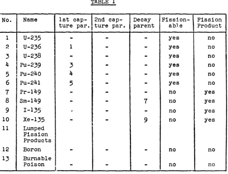
Aooording to the aforementioned rules, and equations (4­1) and (4­2), isotopie ohains of practioal use can be defined.

Two such sets, very simple, but commonly used in diffusion­de­ pletion codes (10­13) are given in Tables 1 and 2.

[image:32.595.68.534.247.602.2]

The standard set, incorporated in CONDOR­3 is the one shown in Table 1. TABLE 1 No.

1

2

3

4

5

6

7

8

9

10 11 12

O

Name U­235 U­236 U­238 Pu­239 Pu­240 Pu­241 Pr­149 Sm­149 I­I35 Xe­135 Lumped Fission Products Boron Burnable Poison 1st cap­ ture par. ­

1

­

3

4

5

­ ­ ­ ­ 1 2nd cap­ ture par. tm M ­ « i ­ « ■ ­ ­ ­ ! •mr ­ Decay parent ­ ­ «· ­ «* ­ m»

7

­

9

­ — Fission­ able yes yes yes yes yes yes no no no no no no Fission Product no no no no no no yes yes yes yes no no ...

The isotopes of the Table 1 (.standard option) excepted, the se­ cular equations (4­1) and (4­2) are solved analytically. All nu­ merical calculations are performed in double precision in order to minimize intermediate roundoff errors.

- 29

Anyway, this method of solution does not set any upper limit to the length of the time-steps.

TABLE 2 No.

1

2

3

4

5

6

7

8

9

10 11 12 13 14 13 16 17 18 19 20 21 Name Th-232 Pa-233 U-233 U-234 U-235 U-236 U-238 Np-239 Pu-239 Pu-240 Pu-241 Pu-242 Pr-149 Sm-149 I-I35 Xe-135 1st group of fission products 2nd group 3rd group of fission products Boron-10 burnable poison 1st Cap-ture par.

-1

-2

4

5

-7

-8

10 11 - --. -2nd Cap-ture par.

-3

*

-9

-mm -ml -Decay | parent

-2

-mm -mm

8

mm mm mm -13 -15 -mm - Fission-able yes yes yes yes

yes

yes yee yes yes

yes

yes

yes

no no no no no no no no no Fission Product no no no no no no no no no no no no yes yes yes yes yes yes yes no no

30 ­

In any case any time­step cart be further subdivided into an arbitrary number of smaller substeps of equal length,in each of which the time­dependent number densities, as well as the concentration­dependent self­shielding factors, are recalcula­ ted but no flux renormalization takes place.

The details about the equations governing the standard chains of Table 1 and their approximate solutions can be found in ref. 15.

V. ­ PROGRAM OUTPUT

^ W ^ i ^ — » — — ¡mmmmt

The program prints out all input data as soon as they are read at any time­step (e.g. control data, library and self­shielding data etc. )

Moreover, the following data are printed, at each time­step:

­ The region and composition average number densities,

­ The weights (grams) of the burnable isotopes and the fuel en­ richments in each composition,

­ The number densities per mesh element in a tabular form, iso­ tope by Isotope (optional),

­ If a shuffling is to be carried out, the preceding items are repeated for the new fuel arrangement,

­ The macroscopic cross­sections per mesh element, namely the cross­sections of neutron and energy production, the diffusion coefficient, the absorption and removal cross­sections (optional), ­ The successive approximations of χ (by the modal expansion

max x r

method), for any level of poisoning in the criticality searches, ­ The eigenvectors « corresponding to the last criticality search iteration after satisfying the eigenvector convergence criterium, ­ The more significant results of the χ = Κ ­­, calculation by

ΙΪ13.Χ 6 1 X

the finite difference method,

- The volume, power, average power density, fission neutron pro­ duction and average density of each region,

- The flux weighted macroscopic cross-sections for each region and group,

31

- The last two items are repeated for the rodded poison re­ gions, lf any,

- Some quantities relating to the power on the mesh stripes

(channels) parallel to the χ or y axis, that is to the stripes of the reactor rectangular domain bounded by two successive rows or columns,

- The average power density per mesh element in a tabular form (optional),

- The volumes per mesh element in the same tabular form (op­ tional),

- The ratio between the average power density at each mesh ele­ ment and the core average power density ("peak-to-average values of the power density) in a tabular form,

- The point fluxes for each group, and the peak-to-average values of the thermal flux (optional),

- The average fluxes per mesh element for each group (optional), These latter values, normalized to the actual reactor power, are used in the calculation of new time-dependent number den­ sities at each mesh element.

The numerical integrations of a function defined at each mesh point (e.g. the group fluxes) are carried out by approximate for­ mulae which can be found in Ref. 14, with many other details con­ cerning the program output.

VI. - PROGRAMMED STOPS

The program stops and prints an appropriate message when one of the following circumstances happens:

- Inconsistency in the input data,

- If both the diffusion coefficient and the logarithmic deriva­ tive are zero for a same group and mesh element,

- If some macroscopic cross-section is negative,

- If the maximum number of iterations by the modal expansion me­ thod is exceeded,

- If the criticality cannot be maintained,

- If the maximum number of outer iterations (finite difference method) is exceeded,

dif 32 dif

-fers from the wanted eigenvalue χ by more than an input va-lue (e.g. 1%), after a criticality search has been carried out. In this case the problem can be restarted using the lo­ gical unit 10 (See Chap. XIV).

VII. - UNIT SYSTEM

- The microscopic cross-sections are to be specified in barn, - The number densities in Szilard =» 10*" nuclei/cm·^,

- The macroscopio cross-sections are in cm" , - The time in hours,

- The energy in Joule, - The power in watt,

o

- The flux in neutrons/cm /sec, - The weight in gram,

- Tne length in cm,

- The power density in watt/enr. VIII. - PROGRAM ORGANIZATION

CONDOR-3 is an "overlay" program constituted by the following links (the decks constituting the link, system library routines excluded, are shown in parentheses).

- LINKO (MAIN, SSVAL, MAFLC3, GRIF03, EXPRI, EXPAND) - LINK1 (AINSUB)

- LINK2 (BINSUB, DELTAX) - LINK3 (CINSUB, MAPC3) - LINK4 (DINSUB).:

The function of these four links is to read, check, reorder and print the input data. Moreover, the program prints out three reactor pictures, one for the regions, one for the initial compositions and one for the rodded regions, and writes on the pertinent unit the data for the RESTART.

- LINK5 (EINSUB)

- The number densities of the time-dependent isotopes are prin­ ted and the fuel shuffling is carried out.

- LINK6 (SETCAL)

33

-LINK7:

The object of this link is alternative to the previous one and is to calculate the macroscopic cross-sections when the library data are to be supplied (calculated) by the program itself.'The decks are not indicated,for this link can be shaped at will of the code's user within rather wide limits. LINK8 (HARCAL):

The macroscopic cross-sections per mesh-element are printed (optional) and the modal expansion calculation is set up. LINK9 (CR0C03, FLØRA, IØLE, IRIS, LØTØ, OLIVIA, INCHA): The criticality search by the modal expansion method is

car-ried out.

LINK10 (EXHARM, IPPØ):

The point fluxes are calculated by the modal expansion method and saved as a first approximation to- the finite difference calculation. Moreover, if a boundary search is dealt with, the moving boundary is settled on the nearest mesh-line. LINK11 (RØDØN):

The coefficients for the finite difference method are calcu-lated.

LINK12 (NEWCAL, CINDER):

The K -f and the point fluxes are calculatee by the finite

dif-ference method (the control parameters, such as the cross-sec-tion or the boundary of a poison, remain as calculated by the modal expansion method).

LINKI3 (ELPRI):

The program calculates the normalization factor, the integrated fluxes per mesh-element, and the power, the average power den-sity, the neutron production per region (these last results are also printed).

LINK14 (WESEC):

The flux weighted macroscopic cross-sections, the flux integrals and several neutron reaction rates are calculated and printed. LINKI5 (ELFI):

34

to the power on the strips (channels) parallel to the coor-dinate axesj the average and the peak-to-average values of the power density at each mesh-element. Moreover, it prints out the point fluxes for each group, the peak-to-average va-lues of the thermal flux and the average fluxes for mesh-ele-ment (optional).. These latter are used in the depletion

cal-culation.

- LINK16 (REDENS, SINBUR, DBURN, SUBÜEP, BBB, SPLIT):

The depletion calculation, that is the calculation of the new values of the time-dependent number densities which are burnt or built up, is carried out at each mesh element, recalcula-ting the self-shielding factors at each substep.

IX. - INPUT DATA PREPARATION

Some remarks of general character must be premised:

A) The maximum number of bytes available to the programmers on the IBM 360/65 is not yet definitely settled and is likely to undergo changes in a near future. Therefore, in view of possible future restrictions of the machine available storage, the limitations of C0ND0R-3 (e.g. the maximum number of groups, of regions, of mesh points and so on) cannot be specified on this report, so they are indicated parametrically.

The numerical /alues of these parameters, for the present ver-sions of CONDOR-3 now running at Ispra, are given in Appendix C, so that future changes of the program restrictions will only imply the uptodating of Appendix C.

B) The correspondence between the logical peripheral storage units used by CONDCR-3 and the physical units of the IBM 360/65 sys-tem (tapes, disks or drums) is not strictly determined but is left widely to the user's choice (see Appendix B ) .

The input data have been divided into 66 card sets (one set may contain one or more cards):

1 - TITLE

One card (18A4):

35

RESTART problems

­2 ­ GENERAL PARAMETERS

One card (24l3):

Col 1­3 NG UNGO) » number of groups Col 4­ 6 NR («sKREG) = number of regions

Col 7­ 9 NCMP (<KCD) = number of compositions

Col 10­12 NPX feKXD) = number of columns (the columns are numbered rightwardly from 1 to NPX)

Col I3­I5 NPY (iSKYD) = number of rows (the rows are numbered downwardly from 1 to NPY)

N.B. ­ It must be NPX»NPY < KPD except for diago­ nally symmetric cases (IDIAG = 1 on card no. 3* columns I6­I8) which have to fulfill only the broader condition:

(NPX + 1) . NPX/2 s; KPD Col I6­I8 NIS U K I S ) =■ last isotope 'number

Col 19­21 NUCL (JSKIV) = number of time­dependent Isotopes.

The time­dependent isotopes are numbered from 1 to NUCL.

Col 22­24 NIF­(<KIF) m number of fuel isotopes. The fuel iso­ topes are numbered from 1 to NIF (ζNUCL)

Col 25­27 NIP (<KIP) = number of fission products. The fission products are numbered from NIF + 1 to NIF + NIP (it must be NIF + NIP ^ NUCL)

If the field 19­21 (NUCL, is zero or left blank, the program automatically assumes the standard nuclide chains of Table 1, with NUCL ■ 13., NIF = 6, NIP « 5 and 2 burnable poisons.

3 ­ OPTIONS

One card (2413):

Col 1­3 NGRINT (^KRINT) = last time­step. The time steps are numbered starting from 0.

36

-beginning life conditions.

Col 4- 6 NRUN = last time-step to be completed (depletion + diffusion calculation) in the present run

(NRUN < NGRINT). If NRUN = NGRINT, the program ends just after the diffusion calculation of time-step NRUN.

If NRUN < NGRINT, the program ends just after the calculation of the time-step (NRUN + 1) number den­ sities and the RESTART data saving and before the reading of new data (buckllngs, control data, li­ brary data, self-shielding factors), the fuel shuffling (if any) and the diffusion calculation. Col 7- 9 JGX geometry indicator for the left side of the reac­

tor (coincident with the y axis). See fig. 6. JGX » 1 x-y geometry, symmetry (zero derivative)

condition at χ = 0

= 2 x-y geometry, zero flux condition at χ = 0 = 3 cylindrical geometry (x = r, y - ζ). The

cylinder axis is at χ = 0.

Col 10-12 JGY geometry indicator for the top side of the reac­ tor (coincident with the χ axis). See fig. 6.

JGY - 1 symmetry condition at y = C = 2 zero flux condition at y =-- 0

Col I3-I5 IPCF = 0 the flux first approximation, at time step 0, is supplied by the program (i.e. is cal­ culated by the modal expansion method), = 1 the flux first approximation is supplied by

a data set (e.g. a magnetic tape). See Chap. XIII,

­ 37

Col 16 ­ 18 IDIAG » 1 The reactor is symmetric about the main diagonal (oriented from the top left corner towards the bottom right one)

« 0 is not symmetric

i

I j

to

r

Σ:

SyMMeTRY A * IS (JCiV = iJ

s ■

-ST

II

>-·

0

*—»

3 -1

u-O Oí UI

Ν

'

*ZEfco FLUX ^ G y . i )

Xft·

X*

\ #

ZtTRO FLUX

1

X -a

U-0

IL/

Ν

Flg. 6

Ccl 19­21 ΙΒΚ = 0 group­independent buckling = 1 group­dependent buckling

Generally speaking, the transverse buckling is as­ sumed to be region­dependent.

Col 22­24 LIBCAL =» 0 the library data (microscopic cross­sec­ tions, fission yields) and the self­shield­ ing data must be supplied by cards

« 1 the aforementioned data are supplied (i.e. calculated at each time­step) by the pro­ gram

Col 25­27 NAX (ÍSKAX) « number of harmonics (wave equation ei­

genfunctions) along the χ axis. See (1­6).

If a criticality search is not dealt with, the value NAX » 1 is advised. On the contrary, if this field

is blank or zero, the program sets NAX = 7·

38

-for a straight K ff> calculation (no criticality

search) and NAY - 7 is the standard value il' a blank or a zero value is punched.

4 - MISCELLANEOUS One card (7E10.5):

Col 1-10 DEL = ô = pointwise convergence criterion for the finite difference calculation of the K - ,

ΰ ΐ i

and fluxes:

l/fe­¿"­ ­ δ

(The same value is used as an eigenvector convergence criterion in the modal expan­ sion calculation)

Col 11­20 HERR » eH = allowed error in the modal expansion cal­

culation:

λΗ ~XD Γ eH

where χ „ and x^ are the eigenvalues (K ff.)

calculated respectively by the modal expan­ sion and by the finite differences. If this field is left blank, the program sets

HERR = 0.01.

If, at any time­step, a criticality search does not meet the above condition, the pro­ gram will give a warning message and will stop at the end of the same time­step. If required, the problem could be continued with a RESTART procedure (see Chap. XIV), eventually after modifying the value of HERR (see Chap. X ) .

5 ­ LIST OF. TIME­STEPS WITH NEW SPECIFICATIONS FOR POINTWISE EDIT

One or more cards (2413), present only if NGRINT > 0, for the spe­ cification of the vector NEDIT(K), Κ « 1, NGRINT, where:

­ 39 ­

» 0 the aforementioned data are not read but they remain the same as in the previous time­step.

6 ­ LIST OF TIME­STEPS WITH NEW BÜCKLINGS

One or more cards (2413) present only if NGRINT > 0, for the specification of the vector NBK(L), L « 1, NGRINT, where :

NBK(l) » 1 the program reads new bucklings (by region and, eventually, by group) after the depletion cal­ culation of the time­step I,

« 0 new bucklings are not to be read at time­step I.

7 ­ LIST OF TIME­STEPS WITH NEW CONTROL DATA

One or more cards (24l3), present only if NGRINT > 0, for the specification of the vector NCT(K), K = 1, NGRINT, where :

NCT(l) = 1 the program reads new control data after the de­ pletion calculation of the time­step I,

» 0 new control data are not read.

8 ­ LIST OF TIME­STEPS WITH A NEW LIBRARY

One or more cards (2¿!I3), present only if NGRINT > 0, for the specification of the vector NTL(K),K «= 1, NGRINT, where:

NTL(I) » 1 the program reads new library data after the de­ pletion calculation of the time­step I,

β 0 no library data are read. All library data keep the last specified values in the previous time­steps.

9 ­ LIST OF TIME­STEPS WITH NEW SELF­SHIELDING DATA

One or more cards (24l3), present only if NGRINT > 0, for the specification of the vector NTS(K), Κ ■ 1, NGRINT, where:

NTS(I) = 1 the program reads new self­shielding data after the depletion calculation of the time­step I,

« 0 no self­shielding data are read.

N.B. 1) The card sets 8 and 9 should be missing if:

40

-2) All data, for which the card sets 5,6,7,8,9 allow new values to be read during the reactor lifetime, are au­

tomatically required by the program at the time-step 0, that is at the beginning of the problem.

10 - LIST OF TIME-STEPS WITH SHUFFLING

One or more cards (2413), present only if NGRINT > 0, for the specification of the vector NFU(K), K « 1, NGRINT. NFU(l) β 1 the program carries out a fuel shuffling before

the time-step I diffusion calculation. The details of each shuffling will be given by the card set

no. 65,66,

» 0 no shuffling at time-step I.

11 - SUBSTEP DIVISION

This set of one or more cards (24l3), present only if NGRINT > 0, specifies the subdivision of each time-step I into NSA(l) sub-steps of equal length. The first card contains:

col 1-3 NSA(l) » number of substeps into which the time-step 1 is divided,

ool 4-6 NSA(2) « ....

and so on, up to NSA(NGRINT)

12 - TIME-STEP LENGTHS

This set, present only if NGRINT > 0, is made up of one or more cards (7E10.5). On the first card:

ool 1-10 DELTAT(1) - length (in hour) of the time-step 1, col 11-20 DELTAT(2) « same for time-step 2.

and so on, up to DELTAT(NGRINT), using as many cards as neces­ sary.

13 - TIME-3TEP POWERS

This set contains one or more cards (7E10.5)· The first card is:

- 41

col 11-20 W(2) « power (watt) for time step 2, and so forth, up to W(NGRINT)

If a straight diffusion-calculation (NGRINT=0) is dealt with, only one card (7Ξ10.5) should be supplied.

col 1-10 W = power (or any arbitrary normalization factor) for the flux normalization.

It is understood that, for an x-y plane reactor, only the power per unit transverse height (watt/cm) is to be given.

Moreover, if the reactor is symmetric about one or both coordi­ nate axes (cylinder revolution axis excluded), only 1/2 or, respectively, 1/4 of the actual reactor power must be supplied.

Finally, we remind that, at any time step K, the fluxes are nor­ malized in such a way that:

G Lx Ly

V

[ i

E*

9i

(x,y) p(x) dx dy = W(K)

where L and L are the lengths of the sides of the rectangular

χ y *

domain under investigation, E~ is given by (3-7) &nd:

/- =» 1 for a plane reactor

P'x' j = 2^x for a cylindrical reactor

14 - γ1 SPECIFICATION

One card (7E10.5) containing the fission spectrum integrals χ (1 β 1,2,...NG) for all grouos.

i NG i It must be χ > 0 and 2 χ > 0.

15 - Δχ - MESH SPECIFICATION (along the x-axis)

Each card is divided into 6 parts [6(Ε9·3,Ι3)] of 12 columns each. Each part is constituted by a floating point field (E9»3) allotted to a value of Δχ(= distance in cm between two succes­ sive columns of mesh points) and by a fixed point field (13) for the column number ("termination point") up to which the

previous value of Ax is extended. All these integer numbers must be specified in an increasing order and the last one must be NPX.

42

of other floating variables.

16 - ΔΥ-MESH SPECIFICATION (along the y-axis)

The same input pattern as before is applied. The last termination point must be coincident with NPY.

N.B. - This set of cards must be omitted in diagonal symmetry problems (IDIAG = 1 on card No. 3)

17 - COMPOSITION - REGION CORRESPONDENCE

Each card is divided into 8 parts [8(213,3x)] of 9 columns each. Each part is constituted by a fixed point field (13) rented to a composition number, another fixed point field (13) for a "termina­ tion point", that is, in this card set, the region number up to which the previous composition is extended and, finally, a 3 co­ lumn blank field (3X).

The integer numbers representing termination points must be given in an increasing order and the last one must coincide with NR. This input pattern will be namend "I sequential expansion form" and will be used for the specification of other integer variables. The compositions are numbered according to the order in which

the correspondent number densities are specified (sec set No. 23;· NUMBER DENSITIES PER COMPOSITION).

18 - REGION DESCRIPTION

The geometric specification of the regions is made through an in­ put pattern which commonly is given the name of "overlay expan­ sion method".

The lay-out of the regions is input by a sequential specification of rectangular blocks of a given region index.

Any of such blocks can cover totally or partially the preceding ones. Each rectangle of the mesh grid (''mesh element") takes the region index of the last occurring block which includes this rec­ tangle. The specification of the rectangular blocks is carried out by inputing as many sets of 6 integers:

col 1-3 ir = region index of the block

­ 43 ­

col 7 ­ 9

C

2

= right column bounding the block (3< C¿ <C

2

<NPX)

col 10­12 r, = upper row bounding the block

col 13­15 r

2

« lower row bounding the block (l«sr, <r

2

<NPY)

col 16­18 these columns are ignored by the program

The specification is continued in columns 19­33, 37­51 and 55­69,

using as many cards as necessary.

19 ­ BLANK CARD

A blank card marks the end of the region lay­out

20 ­ SPECIFICATION OF THE ISOTOPIC CHAINS

This card set, present only if the field 19­21 (NUCL) of card No.2

is not blank or zero, is constituted by NUCL cards (2A4,3l4,3El0.5),

one per each time dependent nuclide, following the order of the

isotope index from 1 to NUCL.

col 1 ­ 8

Isotope name (any alphameric characters)

It is suggested that the name start at column 1

col 9­12 N„ = index of the first capture parent

^1

col I3­I6 Np « index of the second capture parent

^2

col 17­20 N

0

=» index of the decay parent

Ρ

/

­1 ν

col 21­30 χ

=» decay constant (sec )

col 31­40 Atomic weight (g/mole)

col 41­50

ς » "lumping factor" (0< ζ S 1)

If a fissionable nuclide or an individual fission pro­

duct is being described, this field should be left

blank. On the contrary, for a lumped fission product,

it could be ζ = 1.0 or at least, ζ > 0.

We recall that the integers Ν„ , N,„ , Ν must be less than the

^1 (j2. ß

index of the isotope to which they are associated.

21 - COMPOSITION DATA PARAMETERS

One card (2413) containing the following data items:

col 1-3 NEC « number of isotopes whose number densities are

specified per composition (O^NEC^NIS)

col 4- 6 NEMIR « Number of isotopes whose number densities are

given per region (0<NEMIR<NUCL + 1)

44

-RESTART unit.

> 0 the atomic densities of the burnable isotopes per mesh element are supplied by the RESTART unit (see Chap. XIII).More precisely, NSTEP is the time-step number of a previous calcula-tion at which the number densities to be read were recorded on the RESTART unit (see Chap.XII). In this case, the number of rows and columns

(and hence of mesh elements) and the number of isotopes must be the same in both the present and the previous calculation.

col 10-12 NRC = number of compositions for which logarithmic derivatives are specified. (OsiNRC^NCMP)

col I3-I5 IPUN=1 the region averaged atomic densities (calculated by the program) of the first NUCL+1 isotopes are punched on cards (1P7E10.4) at each time-step, before the shuffling.

These punched cards can be used to input number densities per region in other problems.

IPUN=0 no punched cards.

The number densities of the time-independent isotopes, except the first (of index NUCL-t-1), can be specified only by composition. Instead the number densities of the first NUCL+1 isotopes (that is the time-dependent isotopes plus the immediately next one), can be specified either by composition or by region or both.

Also, except for the isotope NUCL+1, they can be specified by mesh element through the RESTART unit. If this last option is checked, it is yet possible to specify number densities per composition but, as for the burnable isotopes, they can be fed into the reac-tor "as fresh fuel" only by a shuffling procedure (see card set No.65). Moreover, only the number densities of the Isotope NUCL+1 can be specified by region. FiréLly, we warn that, after the read-ing of the relevant number densities, all information on the RE-START unit will be lost.