http://www.scirp.org/journal/jectc ISSN Online: 2162-6170
ISSN Print: 2162-6162
Optimization by Thermodynamics in Time
Finished of a Cold Store with Mechanical
Compression of the Vapors
L. Okotaka Ebale, B. Mabiala
*, D. Nkounkou Tomodiatounga
Laboratoire Mécanique, Energétique et Ingénierie, Chaire Unesco en Sciences de l’Ingénieur-Ecole Nationale Supérieure Polytechnique, Université Marien Ngouabi, Brazzaville, Congo
Abstract
This study made it possible to determine by the application of thermodynamics in fi-nished time, the points of instruction necessary to the development of a regulation system for the rationalization of the power consumption in a cold store. These points were obtained by determining the optimal variations of temperature as well to the condenser and the evaporator corresponding to the minimum capacity absorptive by the compressor for a maximum COP.
Keywords
Thermodynamics in Finished Time, Rationalization of Energy, Maximum Refrigerating Power, Optimal Variations of Temperature
1. Introduction
Response to the demands imposed by the market, of the directives related to the ration-al use of energy and the safeguarding of the environment, the design of the current cold stores requires to a certain extent, taking into account of various constraints, in partic-ular: thermodynamic constraints (minimization of the irreversibilities); technological constraints (pressure losses, losses of fluid cooling) and economic constraints (value for money) [1]. The interaction between these multi-field constraints, poses a problem of optimization which can find its resolution in the application of thermodynamics in fi-nished time, which by definition represents the thermodynamics of the real systems whose heat transfers with the tanks (evaporator and condenser) have external irreversi-bilities [2]. In refrigeration industry, this problem results in the maximization of the
How to cite this paper: Ebale, L.O., Ma-biala, B. and Tomodiatounga, D.N. (2016) Optimization by Thermodynamics in Time Finished of a Cold Store with Mechanical Compression of the Vapor. Journal of Elec-tronics Cooling and Thermal Control, 6, 139-152.
http://dx.doi.org/10.4236/jectc.2016.64013
Received: October 29, 2016 Accepted: December 17, 2016 Published: December 20, 2016 Copyright © 2016 by authors and Scientific Research Publishing Inc. This work is licensed under the Creative Commons Attribution International License (CC BY 4.0).
performance of the cold store in other words, the maximization of its coefficient of performance (refrigerating COP = production/consumption [3]). In the cold stores, the production of the real flow of heat is achieved by means of an evaporator; paradoxical-ly, the ideal and reversible refrigerating cycle of Carnot whose refrigerating efficiency is maximum and of which the differences in temperature between the reserves and the fluid of the cycle are infinitesimal, delivers a null heat flow ([4][5][6][7]). However, to deliver a heat flow not no-one, the heat-transferring surfaces and the time of contact with the tanks must be infinite, thus delivering a virtual refrigerating power. Obtaining a real refrigerating power, thus imposes heat-transferring surfaces and total coefficients of finished transfer, differences in temperatures with the finished tanks ([1][8] [9]). Consequently, one obtains the time of contact between the fluid interns and the fi-nished tanks. In addition, the transfer laws of heat of the two tanks make it possible to obtain heat flows according to the conductance and the differences in temperature; they easily allow the determination of the optimal values of temperature at the evaporator and the condenser for a minimal consumption of energy ([2][5][7]).
These optimal values will make it possible for the system of regulation to adapt the operation of the installation to the temperature variations for a COP maximum (refri-gerating COP = production/consumption). The COP in addition expresses the viability of a refrigerating cycle. Optimization will consist in determining the optimal variation of temperature ∆θ0 to the evaporator corresponding to a minimal consumption of
energy to the compressor Wmin for obtaining a maximum refrigerating flow [10][11].
The resolution of the problem will require the development of a system of equations bringing into playing the equations of the energy assessment, entropy and of heat transfer. A transformation of the sizes dimensioned into a dimensional size will facili-tate the mathematical treatment of optimization of the data of the system of equations
0 θ
∆ and ∆θc.
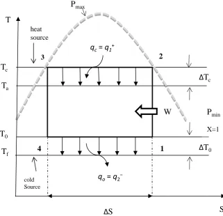
Figure 1 presents the T-S diagram of the endoreversible ideal cycle but exoirreversi-ble, namely that one neglects the internal irreversibilities and one considers only the ir-reversibilities due to the differences of temperature ∆θ0 and ∆θc with the reserves
in heat which are respectively the evaporator and the condenser. The technological and scientific interest is not only the determination of the points of instruction necessary to the development of a system regulation for the rationalization of the power consump-tion by the cold store using a multi-field method but especially taking into account of the irreversibilities inherent in its operation.
2. Material and Method
• Material
The cold store Figure 2 is a group of production of indicated ice-cold water: STANDARD AQUACIATPOWER LD 1800BV R410A. This installation equips the re-frigerating system with the air conditioning of the Bank of central Africa with Brazza-ville.
Figure 1. Diagram T-S (T: the temperature and S: entropy).
Figure 2. Cold store AQUACIATPOWER LD 1800BV standard R410A.
− Refrigerating power: 497.6 kw;
− Power of the condenser: 666 kW;
− Coefficient of performance COP: 2.95;
− Total thermal conductance: 118,657 W/k;
− Temperature of the refrigerant: 280 K;
− Room temperature: 308 K.
• Method for Calculation
The operation of the cold stores with mechanical compression of the vapors has for cycle of reference, the ideal cycle of reversed Carnot. In accordance with the second principle of thermodynamics: heat cannot pass from the cold source of Tf temperature
to the hot spring of temperature Ta without consuming work of the external medium.
The ideal cycle of reversed Carnot is reversible as well internal as (Equation (1))
ex-3
P
maxheat source
T
2
cold Source
P
minS
4
1
Δ
T
cΔ
T
0T
fT
0T
aX=1
W
Δ
S
T
cternal in other words the processes of compression and of relaxation are with constant entropy and the transfer of heat between the fluid and the source is carried out with in-finitesimal differences in temperature. A multi-field analysis of the refrigerating cycle of Carnot highlights the increase in the surface of transfer of heat necessary to the process of vaporization and condensation as the differences in temperature are reduced, is:
Q= ⋅ ⋅ ∆k A T (1)
with: Exchanged total Q = heat; k = heat exchange coefficient; ∆T = difference in tem-perature; A = thermal heat-transferring surface.
When the transfer of heat takes place in extreme cases reversible of way, we have T
T d
∆ − > , then the heat-transferring surface A− > ∞. The run time of the fluid in heat exchangers, (the condenser and the evaporator), tends towards the infinite one. Thus, for a heat-transferring surface of heat and a coefficient of exchange given, we note that the refrigerating power is cancelled.
On the other hand, for an installation producing a real heat flow Q0 to the
evapora-tor, the transfer of heat supposes the existence of a finished difference ∆T in tempera-ture, the cycle of Carnot is irreversible external and the time of contact of the fluid with the sources of heat of surface A limited also has a finished value. The irreversible opti-mization of cycle will consist in maximizing its performance by the maxiopti-mization of its coefficient of performance.
The energy assessment of the installation is given by expression (2):
0
c
W=q −q (2)
And the coefficient of performance of the installation, by Equation (3):
0 0
0
0 0
1 1
COP 1
1 1
c
c c
c
q q
q T
W q q
q T
= = = = ≤
− − − (3)
It is observed that for a mass throughput of the refrigerating agent, the energy as-sessment can be also written in the form of Equation (4):
0
c
mW =m q −mq (4)
If one poses mW =W ; m q c =Qc; mq 0 =Q0, the energy assessment becomes:
0:
c
W = Q −Q (5)
The entropic assessment as for him is written by Equation (6):
0
0 0 0
c c
c
c
q q
T q
T = q =>T = T (6)
The equations of heat transfer to the evaporator and the condenser are given by ex-pressions (7) and (8):
0 0 0 0; Q =k A T∆
0 0 0
Q K T
=> = ∆ (7)
;
c c c c
Q =k A T∆
with Kc=k Ac c ; ∆ =Tc Tc−Ta
c c c
Q K T
=> = ∆ (8)
From two Equations (7) and (8), it results the entropic expression (9):
0 0
c c
Q Q
T = T
(9)
The dimensional notations are declined as it follows:
0
; ;
a o c
c
f f a
T T T
T T T
τ= θ =∆ θ =∆ (10)
The parameters to be taken into account for the optimization of the installation are the following ones: Q0, K, To, Tc.
0 0 0 0 f 0 cte; cteet 0 c 0 c
Q =K ∆ =T K T
θ
= K =K +K = A=A +A (11)The variables to be taken into account for the optimization of the installation are the following ones: Independent variables: θ0 and θc; Dependent variables: K0 and Kc.
The transformation of the dimensioned sizes of the installation into a dimensioned size enables us to obtain the expressions of:
• A dimensional refrigerating power (Equation (12)):
0
0 0 0 cte
f
Q
Q K
KT θ
= = = (12)
( )
0 0
0 0 0
with f where 0;1
K K
Q KT K
K
θ
K= =
• A dimensional calorific power of the condenser (Equation (13)):
(
)
00
0
1 1
c
c c c
f
Q Q
Q K
KT τθ θ τθ
= = − = − (13) 0
with c c a
c c f f c
c
a f
K T T K K
Q K T K T KT
K T T K τθ
∆ −
= ∆ = × × × × =
(14)
• A dimensional mechanical work is:
0 0 0 0 1 c c f Q W
W Q Q Q
KT θ τθ
= = − = − −
(15)
• The coefficient of performance becomes:
0 0 0
1 1 1
1
COPc c
W
Q Q θ τθ
= = − −
(16)
That is to say:
By replacing the notations previously established in the entropic equations, we ob-tain:
0 0
c c
f a c
Q K T
T T T T
∆ =
− ∆ + ∆
(18)
However ∆ =T0 Tfθ0; ∆ =Tc Taθc and Kc =K−K0.
One has:
(
0)
0 0
a c
f f a a c
K K T Q
T T T T
θ θ θ − = − + (19)
(
10 0)
(
(
10)
)
a c
f a c
K K T Q T T θ θ θ − => = − + (20)
By simplifying the room temperature of Equation (20), then by dividing the equation by the coefficient of heat exchange total K, one has:
(
10 0)
(
0)
1c f c K K Q KT K θ θ θ − => = − + (21)
However, 0 0
f
Q Q
KT
= and K0 K
K
= , ones has:
(
)
0 0 0 1 1 1 c c Q K θθ = − θ
− + (22)
In addition, it is known that 0
0 0
0
Q Q Kθ K
θ
= => = Equation (22) is still written:
0 0 0 0 1 1 1 c c
Q Q θ
θ θ θ
= −
− + (23)
In other words Equation (23), can be still written in the form:
(
0)
0 0
1 1 1
1 1 c Q θ θ θ + = − −
(24)
It results from it that:
(
0)
0 0 1 1 1 1 1 c Q θ θ θ = − − − (25)
Consequently after substitution θc inside Equation (17) of the coefficient of
per-formance (COP), we obtain:
(
)
(
0 0)
0 0
0
0 0 1
COP , ,
1 1
1
1 1
1 1
C f Q
Q Q τ θ θ θ θ = = − − − − − (26)
After some simplifying transformations of the denominator COPc of Equation (26):
(
)
0 00
0 0 0 0 0 0 0 0
1 1 1 1 1 1
1 1 1 1
Q Q Q Q Q
θ θ
θ
θ θ θ
− − − = − − + − = − −
(27)
We obtain a final expression COPcirr naturally smaller than that of the cycle of
Car-not COPr
c which is the coefficient of performance of an ideal cycle. The maximum of
the irreversible coefficient of performance is obtained for a minimum of consumption since the production of cold is imposed and thus remains invariant.
2
0 0 0
0 0 0
0 0 0
1 1 1
COP COP
1 1 1 1
1 1 1 1 irr r c c Q Q Q Q τ τ
θ τ θ
θ θ
θ
= = < =
− − − − − − − − (28)
Let us pose 02 0 Q0
θ θ Ψ =
− and let us cancel its derivative
(
)
(
)
2
0 0 0 0 opt
0 0
2
0 0 0
2 d 0 2 d Q Q Q
θ θ θ
θ
θ θ
− −
Ψ = = => =
− (29)
The value which cancels this derivative makes it possible us to obtain the maximum value and consequently the coefficient of performance COPc becomes maximum:
2 0 max 0 0 4 4 Q Q Q
Ψ = =
And max 0 1 COP 1 1 4 c Q τ = − − (30)
opt opt opt opt
0 0 0 0 0 0 0
1 1
0.25; 0.5 because 2
4 2
Q < = Q =K
θ
=>K = =θ
= Q (31)By replacing opt 0 2Q0
θ
= in the expression of θc (Equation (25)), we obtain theop-timal value opt
c
θ
, Equation (32):opt 0
opt
0 0
opt
0 0 0
0 0 0
2
1 1 1
1 1 1 1 4
1 1 2 2
2 2
c
Q
Q
Q Q Q
Q Q θ θ θ = = = = − − − − − − (32)
We can express according to in the form:
opt opt 0 opt 0 1 2 c θ θ θ =
+ (33)
What enables us to obtain:
• minimal a dimensional calorific power (Equation (34)):
min 0 opt 0 0
opt 0 0 0 2 1 1 1
2 1 4 1 4
c c
Q Q Q
Q
Q Q
τθ τ τ
θ
= − = − =
− −
• minimal a dimensional mechanical work (Equation (35)):
min 0
min 0 0 0
0 0
1
1 4 1 4
c
Q
W Q Q Q Q
Q Q
τ
τ
= − = − = −
− − (35)
The coefficient of maximum irreversible performance of the installation (Equations (36) or (37)):
min
0 0
max
1
1 1 4 COPcirr
W
Q Q
τ
= = −
− (36)
max
0
1 >COP
1 1 4
irr c
Q
τ
= =
− −
(37)
If 0 max
1 0 so COP
1
c
Q
τ
= =
− , what corresponds to the output of the ideal cycle of
Carnot.
• and the output of the installation is the report of the performance coefficient of the
ideal cycle of Carnot (Equation (38)):
COP η
COP
irr
r c
= (38)
[image:8.595.231.515.455.676.2]3. Results and Discussion
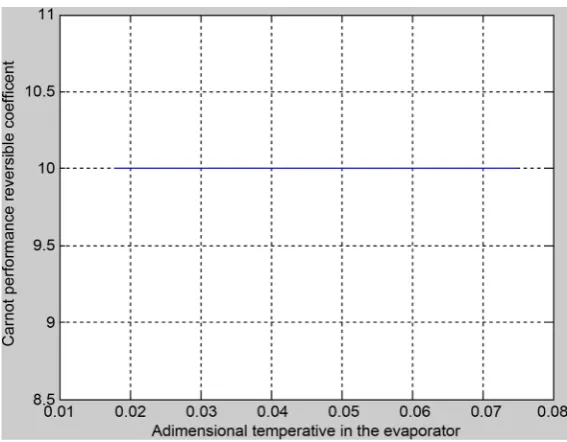
Figure 3 is represented the curve of the evolution of the coefficient of performance of the reversible cycle of Carnot of the installation according to the a dimensional temper-ature θ0 [3][7]. It is noted obviously that this curve has a constant evolution more
especially as heat exchange with the sources of heat (evaporator condenser) are carried
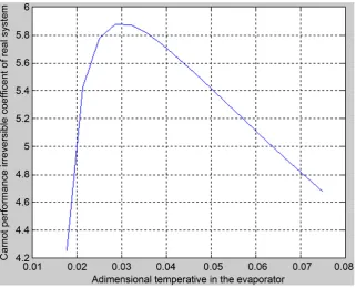
out in an isothermal way, [5] [6] [8]. Consequently, the coefficient of performance C.O.P depends only on the a dimensional report τ = When well even the value of the C.O.P would be maximum compared to that real as Figure 3 indicates it, the refrige-rating flow produced by the installation under the conditions of reversibility remains virtual [5][6]. In opposition to the reversible cycle of Carnot, Figure 4 presents the evolution of the coefficient of performance of the irreversible cycle of Carnot of the in-stallation whose irreversibilities caused by differences in temperature have the evapo-rator and with the condenser produces a real refrigerating flow, Figure 1[1][8]. The evolution of the COP of the installation in function de θ0 is not constant any more.
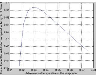
It presents a maximum corresponding has a minimum of energy expense Figure 5. The evolution of the output of the installation compared to the cycle of Carnot represented in Figure 6 also presents a maximum. This situation corresponds to the optimal dif-ferences of temperature =8.38 K having the evaporator and respectively =0.0318 K with the condenser. The power absorptive by the compressor indicates for these same op-timal values a minimal value for the permanent evacuation of the heat flow imposed of the cold room corresponding to a minimum of heat flow evacuated to Figure 7 con-denser. Thus, a distance beyond the optimal point of instruction during the operation of the installation due to the temperature variations involves an increase in the losses (external irreversibility) and implicitly a reduction of the output of the installation.
So that the installation produces a real heat flow Q0=k A T0 0∆ 0 to the evaporator,
[image:9.595.213.535.417.677.2]the transfer of heat imposes the existence of a variation in temperature. However, when this variation of temperature ∆ →T0 0, we have Q0 =0 and the coefficient of
Figure 5. Evolution of a dimensional minimal mechanical work.
Figure 6. Evolution of the installation output compared to the Carnot cycle.
performance COP 0
c
Q W
= becomes null. If this variation ∆ → ∞T0 , energy consump-
tion W to obtain is very high, the coefficient of performance is also null. To maximize the coefficient of performance in our case means a minimal consumption of energy
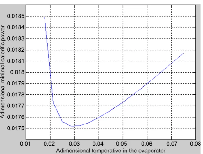
[image:10.595.213.534.350.601.2]Figure 7. Evolution of the dimensional minimal calorific power.
evaporator temperature corresponding to a consumption minimal of energy for ob-taining flow. In substituent the dimensional optimal temperature opt
0 2Q0
θ
= in Equa-tions (15), (17), (25) and (28), we obtain the curve maximum of the real coefficient of performance (Equation (36)) and the minimum of the a dimensional mechanical work curve (Equation (35)); respectively Figure 4 and Figure 5. The expression (34), watch that the minimum of curve of a dimensional mechanical work corresponds at least of the dimensional calorific power curve (Figure 5 and Figure 7), since the refrigerating power is a constant. That is simply explained by the fact why the heating energy eva-cuated with the condenser decreases or increases when the work consumed by the compressor decreases or increases. With regard to the output of the installation com-pared to the cycle of Carnot Figure 6, its pace is similar to that of the coefficient of performance of the real cycle of the installation, for the simple reason that in the report, the denominator is invariable.4. Conclusion
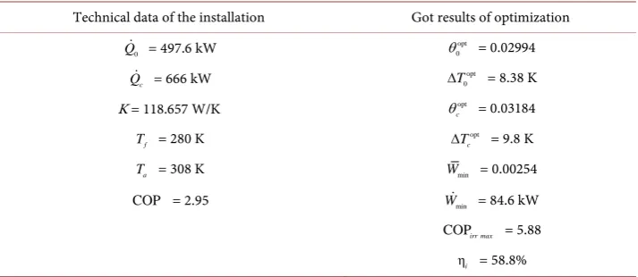
Table 1. Summary of the digital application of the optimization of the power station to ice-cold water.
Technical data of the installation Got results of optimization
0
Q = 497.6 kW opt 0
θ = 0.02994
c
Q = 666 kW opt 0
T
∆ = 8.38 K K = 118.657 W/K opt
c
θ = 0.03184
f
T = 280 K opt
c T
∆ = 9.8 K
a
T = 308 K Wmin = 0.00254
COP = 2.95 Wmin = 84.6 kW
COPirr max = 5.88
ηi = 58.8%
performance 5.88. This coefficient of performance is largely higher than that is pre-sented by the manufacturer 2.95, for the simple reason that in our study we do not take account of the losses caused by the internal irreversibilities. Lastly, to guarantee an op-timal operation of the installation, the system of regulation of this one will have to be programmed according to the points of instruction of the optimal operating ranges.
References
[1] Grosu, L. (2000) Contribution à l’optimisation thermodynamique et économique des machines à cycle inverse à deux et trois réservoirs de chaleur. Thèse de doctorat, Institut National Polytechnique de Lorraine, Université Polytechnique de Bucarest et Nancy. [2] Radcenco, V.T. (1994) Thermodynamique généralisée. Editura technica, Bucarest. [3] Tables et digrammes pour l’industrie du Froid. Institut international du Froid Juillet 1991. [4] Jean-Noël, F. and Julien, E. (2005) Thermodynamique, Base et Application Dunod Paris. [5] Doumenc, F. (2009) Elément de thermodynamique et thermique. Université de Paris VI
2009.
[6] Mathilde, B. (2013) Reconsidération du moteur de Carno. Université de Lorraine, Nancy. [7] Radcenco, V.T. (1992) Eléments de thermodynamique généralisée, irréversibles en temps
fini et vitesse finie. Institut polytechnique de Bucarest.
[8] Okotaka Ebale, L. (1994) Contribution à l’étude de l’optimisation des systèmes de conditionnement de l’air. Thèse de doctorat, Université Polytechnique de Bucarest. [9] Institut international du froid (Ed.) (1990) Le froid et les CCF, compte rendu du colloque
international de Bruxelles 1990.
[10] Grosu, L., Feidt, M., Benelmir, R., Radcenco, V. and Dobrovicescu, A. (2000) Synthèse et perspectives des travaux relatives à l’étude thermo-économique des machine à cycle inverse. ENTROPIE no. 224/225, p. 11-18.
Nomenclature
A: Heat-transferring surface
Ac: Surface of the condenser A0: Surface of the evaporator
BEAC: Bank of the States of Central Africa BP: Low pressure
COP: Coefficient of performance
COPcirr: Coefficient of performance of end or eversible but exoirréversible Carnot
COPcr: Coefficient of performance of end or eversible and exoréversible Carnot
c
T
∆ : Variation in temperature to the condenser
0 T
∆ : Variation in temperature with the evaporator
sc
T
∆ : Variation in temperature of the superheater
sr
T
∆ : Variation in temperature to the subcooler Ψ: Function
max
Ψ : Maximum of the function h: Enthalpy
HR: Relative humidity
K: Coefficient of total heat exchange by convection
c
K : Coefficient of heat exchange by convection with the condenser
0
K : Coefficient of heat exchange by convection with the evaporator
0
K : Coefficient of a dimensional heat exchange by convection with the evaporator
0
opt
K : Coefficient of optimal a dimensional heat exchange by convection with the evaporator
m: Mass throughput
P: Pressure
c
P : Pressure of condensation
max
P : Maximum power
min
P : Minimum power
0
P : Pressure of vaporization PMB: Dead bottom centre PMH: Not high dead
c
q : Calorific production min
c
Q : Heat a dimensional minimal with the condenser
c
Q : Calorific power with the condenser
0
q : Refrigerating production
c
θ : Heat a dimensional with the evaporator S
∆ : Difference in entropy
T: Temperature
t: Time of contact of the fluid with the exchangers (evaporator and condenser)
a
T : Room temperature, outside
ae
t : Inlet temperature of air
as
c
t : Temperature of condensation
f
T : Refrigerating temperature in the cold room
0
t or T0: Temperature of vaporization v: Specific volume
W: Consumed mechanical energy W : Mechanical power
W: Mechanical power a dimensional with the compressor
min
W : Mechanical power a dimensional minimal with the compressor
Submit or recommend next manuscript to SCIRP and we will provide best service for you:
Accepting pre-submission inquiries through Email, Facebook, LinkedIn, Twitter, etc. A wide selection of journals (inclusive of 9 subjects, more than 200 journals)
Providing 24-hour high-quality service User-friendly online submission system Fair and swift peer-review system
Efficient typesetting and proofreading procedure
Display of the result of downloads and visits, as well as the number of cited articles Maximum dissemination of your research work
Submit your manuscript at: http://papersubmission.scirp.org/